1. Introduction
Managing forest resources requires a detailed inventory of forest species and information about changes occurring in the forest ecosystem, in both biotic and abiotic components. The main focus of forest management and nature protection endeavors should be on the monitoring of species composition changes over time, spatial distribution of species, and vegetation conditions [
1]. Forested areas cover large expanses, making them difficult to analyze using traditional methods of creating forest inventory, which also require substantial financial investment [
2]. In addition to purely pragmatic reasons for protecting forests, increased knowledge of forest ecosystem dynamics and relatively high willingness of developed nations to spend resources on nature conservation create a friendly environment for actions aimed at recreating natural forest ecosystems in place of existing forests. Such actions allow for effective protection of forest ecosystem biodiversity and the creation of new habitats that further increase species composition richness [
3]. Existing methods of creating forest inventories use recurring field surveys, which are often supported by analyses of remotely sensed data (in the form of orthophoto maps or other remote sensing products) [
4,
5]. Remote sensing has proven to provide reliable information about spatial distribution of vegetation conditions [
6], biophysical properties of plants [
7,
8], and monitoring of the human impact on valuable habitats [
9,
10], land cover [
11], vegetation communities [
12,
13], and many other topics.
Classification of plant species using remote sensing is a challenging research area, mainly because of the high correlation of spectral reflectance between species [
14] and the small number of variables that control the overall shape of the spectral reflectance curve (chlorophyll a and b content, carotenoids, leaf cellular structure) [
15]. Moreover, leaf spectral properties are also dependent on plant age, phenology of a given species, and climate adaptations [
16]. Masaitis and Mozgeris [
15] have shown that the greatest spectral differences between several deciduous tree species (
Populus tremula,
Alnus glutinosa,
Picea abies,
Pinus sylvestris,
Betula pendula) at the beginning of the growing period exist mainly in the blue and near-infrared (NIR) regions of the spectrum, while in summer shortwave infrared (SWIR) and red regions provide better differentiation [
15]. Most of the spectral features typical of vegetation (such as chlorophyll a and b absorption features, red edge, pigment absorption features) are concentrated in the visible and near infrared (VNIR) part of the spectrum, making VNIR an attractive spectral range for tree species classification [
17]. On the other hand, some works prove the usefulness of the 1000–2500 nm spectral range in tree species classification [
2,
18,
19]. The above reasons necessitate careful selection of spectral bands used in the analysis of plant species.
Recent studies have demonstrated the use of hyperspectral remote sensing methods to gather information about the spatial distribution of forest tree species. Ghosh et al. [
20] presented results of the classification of pine (
Pinus sylvestris), beech (
Fagus sylvatica), two species of oak (
Quercus robur and
Quercus petraea), and Douglas fir (
Pseudotsuuga menziesii) using minimum noise fraction (MNF) transformed bands from a HySpex hyperspectral sensor [
20]. Results have shown similar performance of random forest (RF) and support vector machine (SVM) classifiers after the MNF transformation of data (achieving 94% overall accuracy (OA) in the best case). Graves et al. [
21] reported 62% OA for classification of 20 tropical tree species in Southern Panama. Classes with large numbers of samples have shown the smallest variation in results and the highest accuracy. The authors suggested detailed analysis of classification errors and their sources, with the help of cross-validation methods [
21]. Despite the good results obtained using hyperspectral data, some researchers enrich spectral data with LiDAR (Light Detection and Ranging) data. Among other things, LiDAR data allow identification of individual crowns of trees, which reduces the problem of “mixels” in classification and enables use of an object-oriented approach [
22,
23,
24]. One good example of the synergistic use of LiDAR and hyperspectral data is work by Ballanti et al. [
23]. A comprehensive review of remote sensing use in tree species classification can be found in Fassnacht et al. 2016 [
19].
Artificial neural networks (ANNs) were used relatively infrequently in remote sensing until recently [
25,
26,
27]. According to [
19], only three studies among 129 analyzed studies using remote sensing for tree species classification used ANNs as classification algorithms. The main problem with using ANNs is that they have large computational requirements, but they still have similar performance compared to faster, better known algorithms such as RF and SVM [
19]. While this is true in general, some studies have reported higher accuracy for results from ANNs [
28]. One of the simpler types of ANN is the multilayered feed-forward perceptron, built from at least three layers of interconnected layers of neurons [
29]. Such a network of connected neurons arranged into layers can be seen as a highly concurrent computational system, capable of finding solutions to a given problem [
30]. Typically, training of a neural network is aimed at minimizing the error of a given objective function, and its degree of success in doing so characterizes how capable the network is at providing a correct solution to the problem [
31].
This paper aims to answer the following questions:
Are hyperspectral data and artificial neural networks useful for mapping tree species?
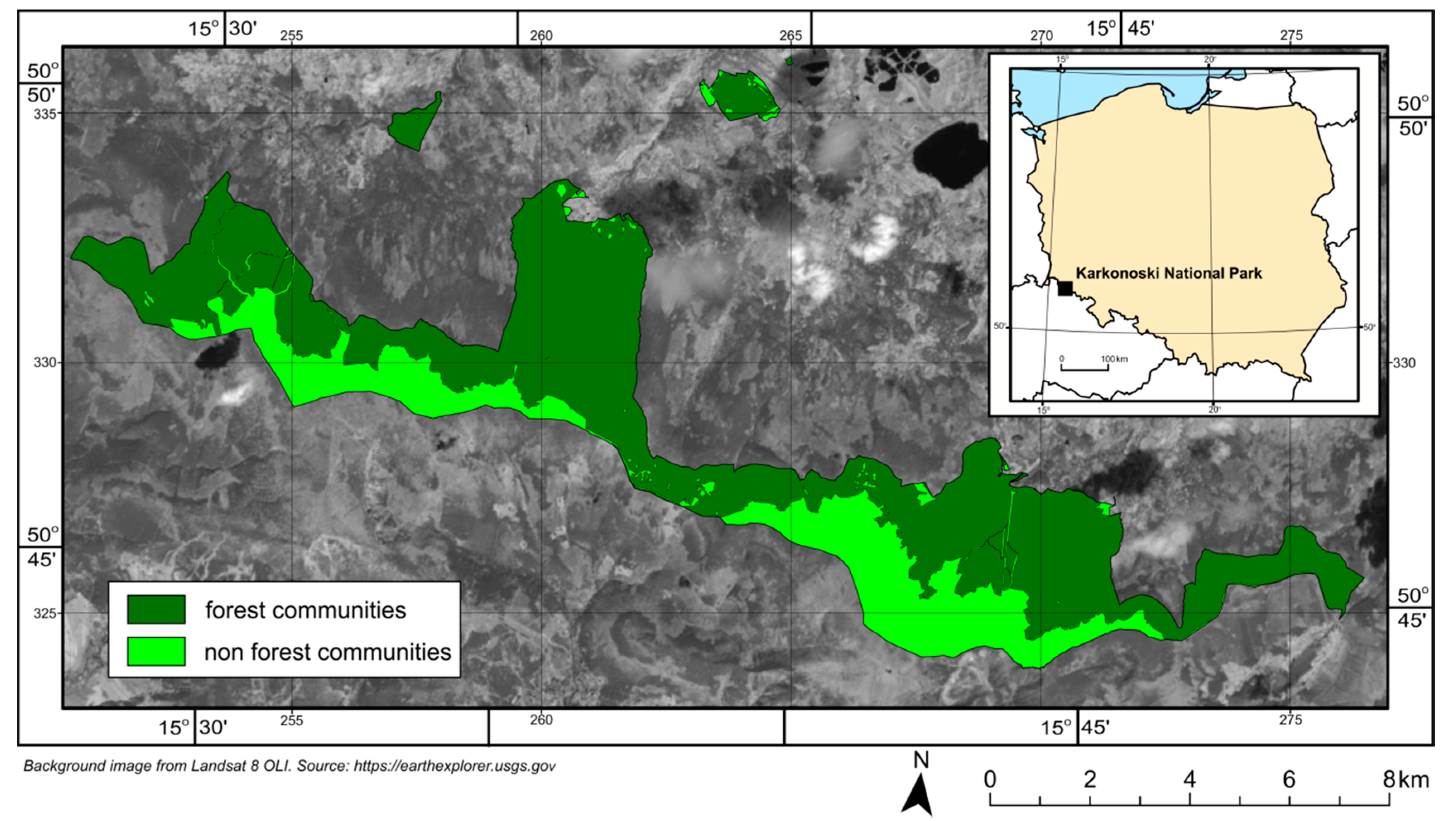
What are the differences between forest inventory and Airborne Prism Experiment (APEX) derived tree species compositions of forest growing in Karkonoski National Park (KNP)?
4. Results
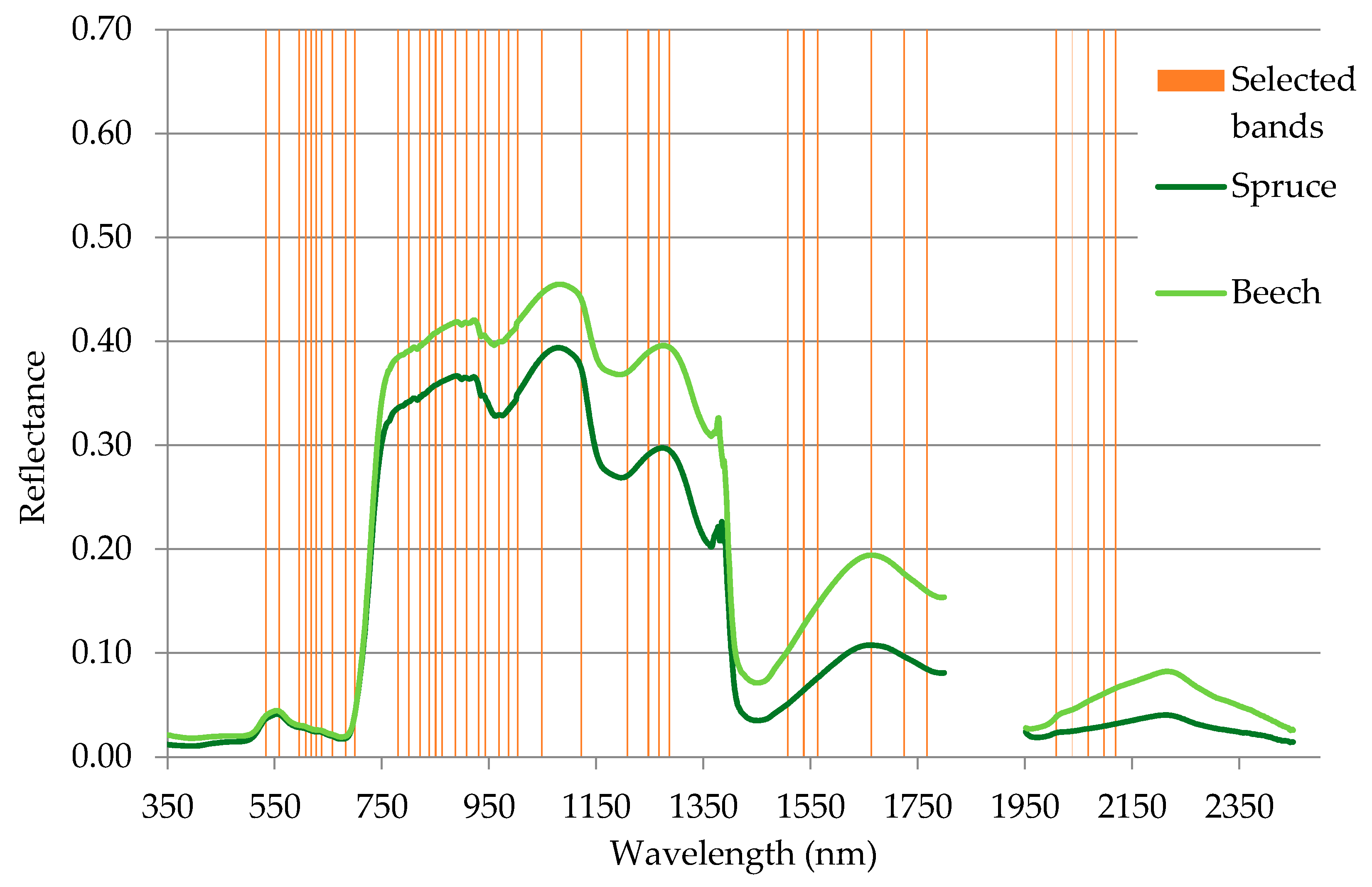
The band selection procedure selected the 40 most informative spectral bands (
Figure 5). Most of the selected bands lay in the VNIR spectral region. In VNIR, the 600–690 nm and 850–1000 nm regions contained the majority of the selected bands. Those regions are associated with light absorption by chlorophyll and increased reflection of electromagnetic waves caused by the cellular structure of leaves. None of the selected spectral bands were located in the red edge region. Spectral bands in SWIR were less often selected, but all of those deemed informative were located in characteristic parts of the spectral curve (associated with absorption features and bending points of the curve). A full list of selected bands can be found in
Table 4.
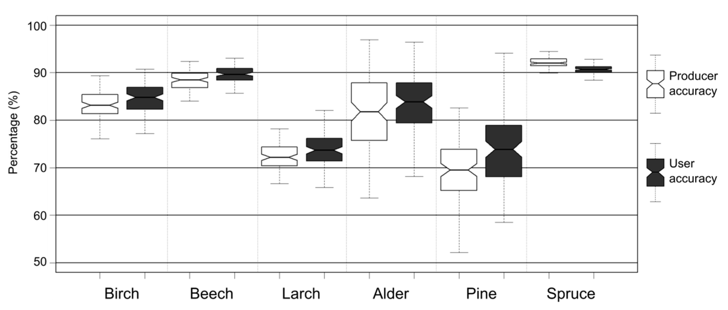
Median overall accuracy achieved by classification was 87%, with median kappa coefficient of 0.81. The classes with the highest median producer accuracy were beech and spruce (88% and 92%), and the classes with the lowest producer accuracy were larch and pine (73% and 69%;
Figure 5). The classes birch and alder acquired 83% and 82% PA, respectively (
Figure 6). The classes beech and spruce had the highest median user accuracy (89% and 91%), and the classes beech and alder achieved around 85% UA. The classes larch and pine had the lowest PA of all classes and achieved 75% median UA. In addition to commonly used accuracy measures, iterative accuracy assessment allows not only singular values to describe various measures to be analyzed, but also distribution of accuracies. Width of distribution and skewness can be used to assess training datasets for spectral homogeneity, show interesting properties of analyzed classes (such as high spectral heterogeneity, which would cause wide distribution of accuracies), or describe how well a given classification algorithm performs on the dataset. Moreover, classes with relatively narrow accuracy distributions can be seen as having been classified with higher confidence than those with wider distributions. Spruce, beech, birch, and larch classes had the narrowest PA distribution (4, 9, 13, and 14 percentage points, respectively), while alder and pine had the widest PA distributions (30 percentage points for alder and 33 for pine). Analysis of UA accuracy distribution shows similar results, with spruce (three percentage points) and beech (six percentage points) having the smallest distribution widths and alder and pine the highest (24 and 35 percentage points).
The created tree species map and nDSM were used to calculate the species composition of KNP by height. This allows for analysis of forest structure in terms of not only tree species, but also tree height. It is worth noting that nDSM does not provide trunk height, but measures tree height from ground level to the top of the tree crown. The species with the largest share of trees over 20 m high is beech (60% are over 20 m high, 27% are between 10 m and 20 m, and only 13% are smaller than 10 m). Larch and alder trees do not have a dominating height class (
Figure 7). This can be explained by the fact that these were classified with relatively low accuracy. It is possible that some pixels classified as larch or alder are, in fact, covered by other tree species, particularly beech or spruce. The effects of 1980s pollution and a bark beetle outbreak can best be seen in the results for spruce. Only 47% of spruce trees are over 20 m high, and 41% are smaller than 10 m. This may give an estimate of the amount of regrown spruce after old forests were cut down to combat the pest outbreak or died due to soil poisoning and air pollution. More than 50% of birch trees in KNP are under 10 m high, 36% are between 10 m and 20 m, and the remaining 12% are above 20 m. This seems to be in line with birch’s growth patterns. Birch is typically one of the first tree species to occupy new areas (such as forest clearings), and is then replaced by other tree species more adapted to a given habitat, but not so expansive.
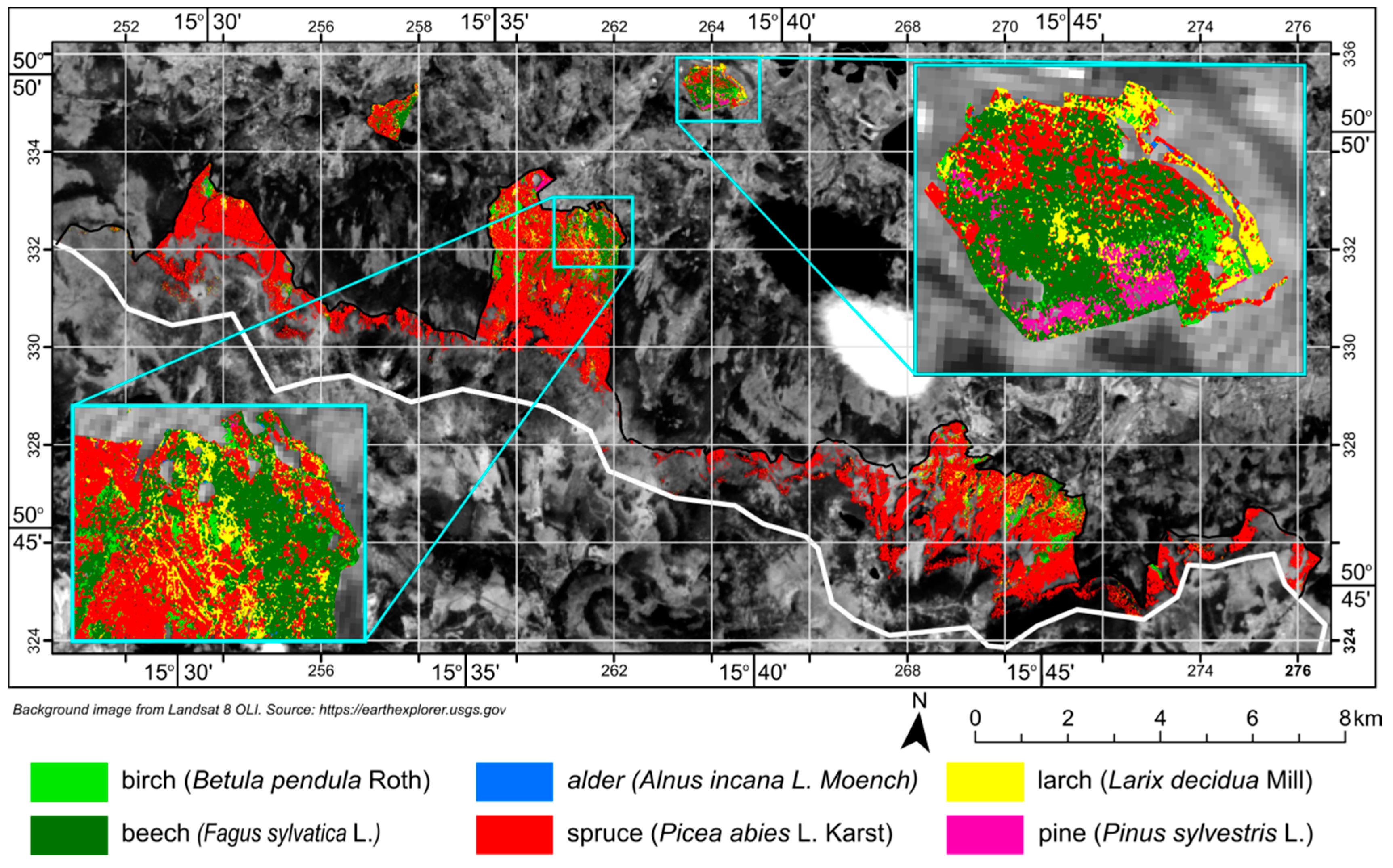
The tree species map (
Figure 8) created from classified APEX scenes was compared with the most recent forest inventory data. Comparing those two datasets can be an interesting point of discussion on the accuracy of remote sensing products and existing datasets. As seen in
Table 5, forest inventory data and classification results agree most closely for the share of birch, larch, alder, and pine in overall forest tree species composition. The greatest discrepancies exist for beech and spruce. Classification results suggest that beech trees comprise more than 10% of all trees, compared to the 4% indicated by the forest inventory. On the other hand, classification results show a lower share of spruce in forest composition as compared to the forest inventory data.
5. Discussion
When comparing the present classification results with those obtained by other researchers using remote sensing data, the data and classification algorithm used must be taken into account, as well as the number of classes determined by individual authors. This mainly relates to the spatial and spectral size of pixels, because large pixels register not only trees, but also surrounding shadows or other objects around or even under trees. Such “mixels” make correct interpretation of the results difficult. Too small a pixel is also not optimal because it registers the area between individual branches, thus introducing artifacts.
Works on tree stand classification are often practical in nature and aim to map the spatial distribution of tree species [
2,
46], although there are also those that treat the classification of tree species as a nontrivial problem on which they test different data-processing methods and classifiers [
22].
In this study, producer accuracy was 93% for the spruce class (
Picea abies L.) and 78% for pine (
Pinus sylvestris L.). In a work by Dalponte et al. [
47] the PA was, respectively, 97% and 95% for spruce (
Picea abies L. Karst) and pine (
Pinus sylvestris L.) classes, and 71% for other species of deciduous trees [birch (
Betula spp. L.) and poplar (
Populus tremula L.)] using an SVM algorithm. Comparing the results of the quoted work, similarly high accuracy was obtained for the spruce class, although the pine class was not classified with high accuracy. In this case, the spatial extent of the occurrence of pine in KPN is of great importance, as it makes it considerably more difficult to select a large set of samples. The author of this paper obtained an average producer accuracy for all broadleaf tree species of 88%, which is higher than the 71% of Dalponte et al. [
47]. An overall accuracy above 80% is not uncommon in forest stand classification, which justifies the use of remote sensing techniques, and hyperspectral remote sensing in particular, to support the mapping of tree species. The vast majority of works focus on classifying only a few species of trees, although there are also those that classify more tree species [
17,
21,
48].
While this work shows good performance of an ANN classifier, previous works were not so successful. In their research, the Feret and Asner team [
48] attempted to classify 17 species of tropical trees growing in Hawaii and achieved decidedly poorer results, ranging around 40% OA despite using artificial neural networks in the MATLAB software (MathWorks, Inc., Natick, MA, USA). These lower results may attest to the greater spatial diversity of tropical tree species. A comparable pixel size and significantly lower accuracy (than the 87% obtained in this work, but with 17 classified tree species) confirm the need for a well-thought-out strategy for selecting learning parameters for ANN. Data from an APEX sensor has already been used to classify tree species using hyperspectral data. A team led by Tagliabue [
18] classified five tree species in Lorraine (hornbeam
Carpinus betulus, two species of oak
Quercus petraea and
Quercus robur as a single class, lime Tilia, and spruce Pinus) using APEX data with 3 m spatial resolution. The APEX data were acquired at the beginning of September. The work used a maximum probability algorithm as the classifier and all acquired spectral channels. The classification had an overall accuracy of 74% and a kappa coefficient of 0.63. The lowest producer accuracy was for lime (71%) and hornbeam (70%), and the highest for pine (80%) and oak (85%). User accuracy ranged from 61% (oak class) to 86% (hornbeam class). Some authors have suggested using higher spatial resolution data or images from a different season [
18]. This work proves that this is not necessary, on the condition that the data and the classification algorithm are appropriately selected. When considering the subject of forest stand classification, it is worth comparing results against those obtained for an area where similar tree species occur. Lee et al. [
24] obtained very good results when classifying tree species using an SVM algorithm in a forest in Oxfordshire, England. Accuracies of over 90% for beech (
Fagus sylvatica) and larch (
Larix decidua) show that it is possible to classify a larch class better than is shown in the present work (76% in the best iteration). The low accuracy for the larch class can be explained by how trees of this species occur in KNP (singly or in small groups, usually planted in a line) and features of its crown (sparse). This makes it difficult to obtain good samples and to correctly classify trees of this species in an image, because it is difficult to find a pixel that is not a mixel of the crowns of larch and other tree species. It is worth mentioning that Lee et al. [
24] used channels after PCA transformation and LiDAR data, which significantly improved the results (increasing OA from 85 to 91%). Due to the dataset used in the present work (imperfections in atmospheric correction caused the spectral characteristics of the same object to be different in two different scenes), images after PCA transformation were not used, which could have led to classification of some classes being worse than anticipated. Comparing the results with the literature, they are in line with the results obtained by other scientists (
Table 6), especially considering that few papers have addressed the classifying of tree species in an area as large as KNP.
Tree species distribution maps derived from hyperspectral data exploit spectral differences among species more than tree crown texture and shape to properly assign labels to pixels. While very effective, hyperspectral data collection is mostly limited to aerial sensors. This is an obvious limiting factor in terms of both the area covered by images and cost. On the other hand, very high-resolution multispectral sensors located on satellites can provide high-quality data for most of Earth’s landmass at reasonable cost. Work by Zeng et al. [
49] showed the use of multispectral Advanced Land Observation Satellite (ALOS) images for classification of six tree species (Chinese fir, Masson pine, Fujian cypress,
Schima superba,
Michelia macclurei, and tung) in Jiangle Forest Farm within the city of Sanming, Fujian Province, China. The sensor spectral bands had a 10 m spatial resolution, which was boosted to 2.5 m by use of pansharpening, performed using the ALOS 2.5 m panchromatic band. Using a combination of image segmentation, object-based classification techniques, and rough set theory–based classifiers, researchers were able to achieve classification results with 80% OA and 0.76 kappa coefficient, outperforming the nearest simple neighbor classifier. Pu and Landry [
50] managed to classify seven tree species (
Quercus geminata, Q. laurifolia,
Q. virginiana, pine, palm,
Cinnamomum camphora,
Magnolia grandiflora) growing in urban areas of Tampa, Florida, USA, using high-resolution IKONOS and WORLDVIEW 2 (WV2) satellite images. IKONOS images had five bands (four spectral bands with 4 m spatial resolution and one panchromatic band with 1 m spatial resolution), while WV2 had nine bands (eight multispectral bands at 2 m spatial resolution and one panchromatic band at 0.5 m spatial resolution). Both satellites provided bands collected in the VNIR spectral range. Linear discriminant analysis (LDA) and classification and regression tree (CART) classification algorithms were used. Classification created using IKONOS data achieved 57% OA and 0.47 kappa coefficient, while those made on WV2 data achieved 62% OA and 0.53 kappa coefficient. In conclusion, WV2 data were proven to be better for species classification thanks to higher spatial resolution and four additional spectral bands that IKONOS lacked. Classes that were classified above 80% PA were
Quercus geminata for IKONOS data and pine and palm for WV2 data. Typically, when using high-resolution multispectral data, researchers perform various transformations of spectral bands to create new, potentially helpful features [
49,
50]. While multispectral data–derived tree species distribution maps have worse quality than those based on hyperspectral data, the literature suggests that use of submeter red-green-blue (RGB) images coupled with LiDAR data can be an interesting and competitive alternative. A study by Deng et al. [
51] managed to classify four tree species (
Pinus densiflora,
Chamaecyparis obtusa,
Larix kaempferi, and one class containing all broadleaved trees) using a quadratic SVM classifier. For their study, they acquired 0.25 m spatial resolution RGB images and LiDAR point cloud with density ranging from 13 to 30 points per m
2. Classification based on only RGB images achieved 76% OA, while including LiDAR-derived products increased OA to 91%.
The overall accuracy of the classification of tree species can be considered very high (median 87%). This is partly a result of the high producer accuracy for the classes represented in the majority of sample pixels used in the classification (beech and spruce). A more balanced view of achieved accuracy is offered by Fassnacht et al. [
19] and Ghosh et al. [
20]. In both works, for each classified tree species, the authors decided to draw an equal number of reference pixels that, after being divided into a training set and a test set, were used for training the classifier and as a validation set. This approach can avoid inflation of the general accuracy index, which, in the case of the above method, is the simple arithmetic mean of the classes’ producer accuracies. In both works, it was decided to choose 60 pixels per class. Despite the aforementioned advantages of using a set of reference data samples with equal numbers per class, some works feature very unbalanced numbers of samples for classes [
52,
53]. For example, Lee et al. [
24] used 636 reference pixels for the ash class (
Fraxinus excelsior), 255 for larch (
Larix decidua), and 186 for birch (
Betula spp.), obtaining an overall accuracy of 91%. A similar state of affairs is to be found in this work, where there are quite large differences in the sizes of samples for individual classes (2677 reference pixels for spruce, 685 for larch, and 90 for alder).
The researchers classified eight tree species (sequoia (
Sequoia sempervirens), Douglas fir (
Pseudotsuga menziesii), laurel (
Umbellularia californica), oak (
Quercus agrifolia), alder (
Alnus rubra), willow (
Salix lasiolepis), eucalyptus (
Eucalyptus globulus), and horse chestnut (
Aesculus californica)) growing in Muir Woods, CA, USA, using an AISA Eagle scanner. In addition to spectral signature, they included a tree crown model in the classification. The classified image obtained an overall accuracy of 95%, and all classes except for willow (58%) obtained a producer accuracy above 90%, while only two classes had a user accuracy below 92% (oak: 67%, willow: 84%). This is convincing evidence for including LiDAR data in forest stand classification, on the condition that the desired data are extractable [
23]. In this work, it was decided not to include LiDAR data as an additional predictor, due to the fact that LiDAR data were collected earlier in 2012 than spectral data. While LiDAR data can be helpful in tree species classification, our observations made us reconsider using them. First of all, the forests of KNP are actively reshaped, which includes the creation of new forest clearings. Comparing RGB APEX images with LiDAR-derived data (such as DSM), we noticed that several places that were clearly visible as forest clearings on APEX scenes were counted as forested with tree height more than 10 m on DSM. This suggests that those areas were cleared between LiDAR data collection and APEX data collection. It is preferable to use LiDAR data obtained at the same time as spectral characteristics. The use of out-of-date LiDAR data could significantly distort results.
Gathering field data is a very costly task and requires good logistical preparation [
19]. Whether for classification or for other studies using remote sensing data, the in-field data collection stage is certainly very important. Having access to maps, orthophoto maps, and data from various government institutions and private companies does not remove the need to at least inspect the research area. Ideally, field studies should be conducted at the same time as imaging. Depending on resources, some authors carry out fieldwork in the same month as the execution of imaging, supporting their fieldwork with data from state institutions and maps [
2]. Other researchers use data from state institutions and maps without conducting fieldwork [
19]. Naturally, the need to carry out field studies depends on the research area. Areas that are well mapped with up-to-date data (e.g., managed forests) do not require extensive field research, as opposed to sparsely mapped areas with out-of-date data. The classification of species of trees can use field data collected after overflight because of the slow rate of natural changes in the forest and the fact that large and fast changes (felling, windthrow, etc.) are very easy to spot in the field. Of course, in the case of data collection for classifying communities that only occur during a certain part of the year, field tests should be carried out at the time of overflight in order not to falsify the results. In this work, it was decided to conduct a series of field studies for the purpose of gathering reference data for classification. The field studies took place one and two years after APEX imaging. Therefore, during data collection, areas were avoided that were actively being transformed or where cursory inspection detected changes (removed trees, remaining felled trunks) that could have occurred between overflight and field research. During the preparatory work, available maps and an orthophoto map were used to determine the area for field research.
Significant differences (mainly for spruce and beech) between forest inventory and our results can be explained by several reasons. First of all, we decided to use forest mask, which excluded from our analysis areas covered by vegetation smaller than 2.5 m. These excluded areas occupied by saplings and small trees, which would be included in forest inventory [
54]. Moreover, by using forest mask, forest areas included in classification covered about 2027 ha, while officially, forests in KNP cover an area of 4022 ha [
33]. This rather large difference might explain the differences between forest inventory and our results. A second probable cause of differences might be the method of creating forest inventory. Forest inventory in KNP is created using a network of measurement plots. Measurement points are distributed in 200 × 300 m grids [
54]. This rather coarse resolution (but reasonable, considering cost constraints) might bias forest composition toward the most commonly occurring tree species (spruce). High accuracy measures for classes that were noted to have the highest differences in forest composition (spruce and beech) seem to invalidate claims that those differences are the result of an inaccurate tree species distribution map acquired in our work. Differences between tree species maps created using hyperspectral remote sensing and forest inventory data were also reported by Sommer et al. [
17], where the greatest discrepancies were observed for spruce, fir, maple, and birch (39, 15, 8, and 7 percentage points, respectively).
The use of artificial neural networks in remote sensing is not widespread [
19]. This is mainly due to the difficulties in using them and the fact that other classifiers, such as SVM and RF, provide comparable results with much less work. The process of optimizing an artificial neural network’s learning has a large influence on the final result [
48], and it is only one of many things that need to be done to get a good result (others are selecting the architecture, choosing the learning algorithm, and finding the balance between sensible learning time and results). Using the nnet package, which is available for the R program, showed that artificial neural networks can successfully be used in classification tasks. The wealth of additional subprograms available for R allows the entire processing chain to be transferred to one place. In light of these facts, nothing stands in the way of extending the scope of ANNs in remote sensing. It is also worth analyzing whether the use of “deep-learning” networks in hyperspectral remote sensing cloud cover during the aerial pass may affect the results.


