Remote Sensing Images Stripe Noise Removal by Double Sparse Regulation and Region Separation

Abstract

Stripe noise removal continues to be an active field of research for remote image processing. Most existing approaches are prone to generating artifacts in extreme areas and removing the stripe-like details. In this paper, a weighted double sparsity unidirectional variation (WDSUV) model is constructed to reduce this phenomenon. The WDSUV takes advantage of both the spatial domain and the gradient domain’s sparse property of stripe noise, and processes the heavy stripe area, extreme area and regular noise corrupted areas using different strategies. The proposed model consists of two variation terms and two sparsity terms that can well exploit the intrinsic properties of stripe noise. Then, the alternating direction method of multipliers (ADMM) optimal solver is employed to solve the optimization model in an alternating minimization scheme. Compared with the state-of-the-art approaches, the experimental results on both the synthetic and real remote sensing data demonstrate that the proposed model has a better destriping performance in terms of the preservation of small details, stripe noise estimation and in the mean time for artifacts’ reduction.

1. Introduction

The remote sensing image plays an important role in environment monitoring, resource monitoring and military and battlefield situation observations [1,2,3]. However, the output of sensing images often suffers from stripe-like noise, which seriously degrades the image’s visual quality and also yields a negative influence on high-level application, such as target detection and data classification [4,5,6,7]. Due to the inconsistent responses of detectors and the imperfect calibration of amplifiers, the gain and offset of true signals are various, producing stripe noise on Moderate Resolution Imaging spectrometer (MODIS) data and hyperspectral images. The MODIS data covers 36 spectral bands ranging in wavelength from 0.41 $\mathsf{\mu }$m to 14.4 $\mathsf{\mu }$m. Three typical striped images are displayed in Figure 1, and the stripe effect is obvious by zooming in. This noise is periodic for 10 pixels for the detectors’ calibration errors and the charge-coupled device array scanning forward and reverse across-track [8,9].

In recent decades, a large number of destriping algorithms have been discussed for remote sensing images and can be grouped into several categories by various mechanisms, such as the filtering-based methods, statistics-based methods and optimization model-based approaches.

The statistical-based methods include a moment matching algorithm [8,10,11] and midway equalization algorithm [12]. Moment matching techniques assume that the sensors’ outputs have the same statistical characteristics including mean and deviation, and they set all sensors’ output to a reference one. In [11], the authors proposed a piece-wise approach to remove the irregular stripes by local statistical information. The midway equalization method supposes that the histogram distribution between neighbouring columns is similar and a local midway histogram is computed for the current column. The performance of these methods is limited to the hypothesis, which does not always hold, that when a structure exists along the stripe direction, the statistics between neighbouring columns are distinct.

Filtering-based algorithms remove stripe ingredients by a type of filter in the transformed domain after discrete Fourier transform [13] or wavelet decomposition [14,15,16]. A regular periodic stripe exhibits a particular frequency component, and can be easily identified in the transformed domain. Unfortunately, blurring effects and artifacts may appear when filter models are not well designed, and some textures similar to stripe are also prone to be smoothed, as they are likely to be identified as the noise.

Recently, optimal model-based destriping methods have attracted many endeavours’ interest and numbers of models have been formulated. People introduce prior knowledge of noise and ideal remote sensing images into an energy function to recover the latent content. The unidirectional variation model (UV) was first proposed by Bouali et al. [17]. They formulated a differential optimal model based on the stripe noise’s direction property that stripe noise only affects the gradient information along one direction and will not change it in another direction. To overcome several limitations [18] of the UV model, improvement algorithms were subsequently designed. Zhou et al. [19] designed a hybrid unidirectional total variation (HUTV) model that combines a $l_1$ data fidelity term and gradient fidelity term aiming to remove stripe noise of various intensities. To distinguish the noise from the texture and edge, Zhang et al. [18] proposed a structure guided UV model. Wang et al. [20] utilized difference curvature to extract the spatial information, and formulated a spatially weighted UV model. The authors in [21] combined the UV model and framelet regularization to preserve the detail information while removing the stripe noise. In [22], the UV model was converted to a least square problem by an iteratively reweighted technique that was easy to implement. Regarding the destriping problem as an ill-posed inverse problem, the (column) sparsity property and low rank property of the stripe noise served as a regularization to improve the stripe estimation performance in [23,24,25]. Chen et al. [26] combined the group sparsity constraint and total variation regularization to remove the stripe noise and preserve edge information. Dou et al. [27] proposed a directional $l_0$ sparse model for stripe noise removal. Some researchers also exploited the high spectral correlation property among the different bands in hyperspectral data to recover the latent image [28,29,30]. With the rapid development of deep learning techniques, the deep convolutional networks based destriping methods [31] were proposed and showed a competitive stripe noise removal ability in the infrared image. However, their framework was designed for weak stripe noise only, and could not be suitable to the strong stripe noise.

In summary, most existing methods can recover clean images directly or indirectly from degraded images based on the stripe noise property, such as gradient information and sparsity characteristics. However, a common problem existing in recent research efforts is that the details or structure along the stripe direction can not be recognized well and probably get confused with the stripe noise, resulting in an oversmoothing effect. In addition, once the data are corrupted by serious stripe noise, the output can not recover the scene well and often suffers from stripe artifacts. We in this paper attempt to alleviate the two problems. The sparsity property not only exists in the spatial domain, but also exists in the gradient domain. Thus, we here present an optimization framework that utilizes a double sparsity counting scheme to estimate the stripe noise more completely to protect the details from being destroyed during the destriping process. A region separated processed strategy is adopted here. Specifically, for the heavy stripe corrupted area, we utilized the texture diffusion method only on the direction across the track to inpaint them. Extreme dark or extreme bright areas were kept the same as the original. For the normal stripe noise corrupted area, the noise was estimated by the stripe’s characteristics.

The remainder of this paper is organized as follows: Section 2 introduces some properties of stripe noise. Section 3 presents the proposed weighted double sparse destriping model. Section 4 discusses the experimental results and comparison analysis. Section 5 presents some discussions about the proposed model. Finally, conclusions are provided in Section 6.

2. Stripe Noise Properties Analysis

2.1. Stripe Variation Property

In most model-based destriping methods, the output of a noisy image is formulated as an additive noise formulation [21,24,32], as follows:

$$\begin{array}{c}{Y}_{u,v}=X_{u,v}+S_{u,v},\end{array}$$

(1)

where X and Y denote the unknown desired image and observed degraded image, respectively. S represents the stripe noise and $(u,v)$ is the spatial coordinate in an image. The purpose of a destriping technique is to estimate a clean image X from Equation (1). It is a typical ill-posed inverse problem and some additional regulations are desired to constrain the solutions. In this paper, we assume the stripe direction is along the u-axis.

Stripe noise obscures image details and sometimes even destroys the texture, which poses quite a challenge to recover the real signal, as shown in Figure 1. Fortunately, this type of noise has a good directional property, for it usually only appears along one direction, resulting in the gradient across the stripe direction being far greater than that along the stripe, as illustrated in Figure 2. This property can be expressed by:

$$\begin{array}{c}\frac{\partial Y}{\partial u}\ll \frac{\partial Y}{\partial v}.\end{array}$$

(2)

Based on this property, the unidirectional variation (UV) energy model [9] is formulated as:

$$\begin{array}{c}E(X)=T{V}_u(Y-X)+\lambda T{V}_v(X),\end{array}$$

(3)

in which $T{V}_u(X)=\underset{\mathsf{\Omega }}{\int }(|\frac{\partial X}{\partial u}|)dudv$ is the total variation of X along the u-axis, and $\lambda$ is the regularization parameter to determine the smooth degree on the v-axis. The UV model (3) attempts to keep the variance of the destriped image X along the u-axis with that of the corrupted image, while reducing the variance across the stripe direction on the v-axis. It seems reasonable, yet there are two shortcomings with the UV model. First, it is prone to producing artifacts when the noise intensity is so serious that it damages some texture structure. Second, certain small details are easily prone to be smoothed out during the iterative procedure when $\lambda$ is set to be large.

2.2. Stripe Structure Property

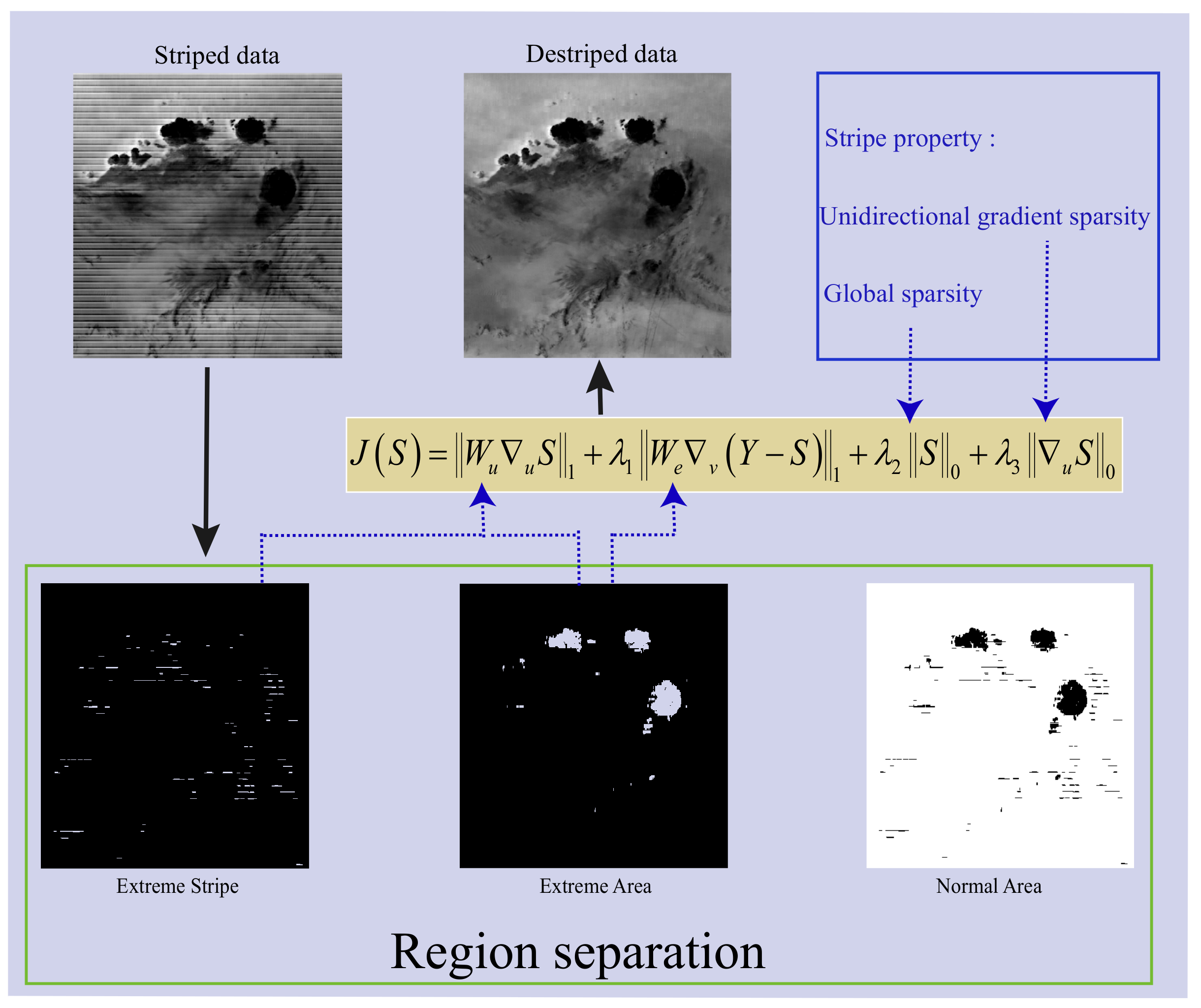
Stripe noise presents a particular structure in which there are many zero elements in stripe-free regions, as different from random noise. In view of this fact, the authors in [24] adopted the $l_0$ norm as a regulation to constrain the noise matrix S:

$$\begin{array}{c}{R}_1(S)={\parallel S\parallel }_0.\end{array}$$

(4)

Although $l_0$ norm provides more zero elements in S, the nonzero elements are distributed randomly, according to the definition of $l_0$ norm. As a result, the non-stripe ingredients are also probably to be treated as noise, causing the details’ smoothing affects. Furthermore, in case of a great proportion of stripe noise, the $l_0$ norm constraint is unreliable. Observing the noise matrix, we discover that the gradient of S along the stripe direction u also exhibits significant sparsity characteristics, no matter the proportion of noise. The regular stripe noise particularly exhibits this property in evidence, i.e., all zeros in matrix ${\mathsf{\nabla }}_{u}S$, regardless of noise levels and proportion. Accordingly, a unidirectional gradient sparsity regulation is expressed by:

$$\begin{array}{c}{R}_2(S)={\parallel {\mathsf{\nabla }}_{u}S\parallel }_0.\end{array}$$

(5)

3. Methodology

Based on the above analysis, we first present the double sparse UV model (DSUV), which is also introduced within the variation framework. Taking advantage of the double sparsity feature of stripe noise, i.e., the signal sparsity and unidirectional gradient sparsity, combined with the variation property, the DSUV model is formulated as follows:

$$\begin{array}{c}J(S)=\parallel {▿}_u{S\parallel }_1+{\lambda }_1\parallel {▿}_v{(Y-S)\parallel }_1+{\lambda }_2{\parallel S\parallel }_0+{\lambda }_3{\parallel {▿}_{u}S\parallel }_0\end{array}$$

(6)

in which ▽ denotes the gradient operator, ${\parallel ·\parallel }_0$ is the $l_0$-norm counting the number of non-zeros in a matrix, and ${\parallel ·\parallel }_1$ is the $l_1$-norm, which summarizes all elements’ absolute values. In model (6), the front part is the UV minimization. The rear part measures the global sparsity of stripe noise S and the unidirectional gradient. The variable ${\lambda }_1$ stands for the variance parameter and ${\lambda }_2,{\lambda }_3$ are the sparse counting parameters. The three regularization parameters balance the four constraint terms together. After S is estimated from model (6), the desired image X will be obtained by subtracting S from degraded image Y. The WDUV extracts the stripe component from the whole image. However, distinct areas with different features should be processed separately, and we analyse it next.

3.1. Region Separation

Many destriping techniques assume that stripe noise presents in the whole column on an image, which is not always true. In some extremely dark or too bright areas, stripe noise is saturated and noise in these regions is almost zero. Therefore, it is not necessary to further estimate noise in these areas. Nevertheless, if an area’s extreme values were generated by a strong stripe, we should recover these elements. Here, we name these areas strong stripe area (SSA), also called the extreme stripe area. Therefore, distinct extreme area (EA) and SSA are necessary. An example of SSA and EA is illustrated in Figure 3.

In this subsection, a simple and effective method for detecting and distinguishing EA and SSA’s method is proposed. It is based on the stripe noise’s property. Take the extremely dark area detection, for example. In both the SSA and EA, grey values are all close to zero and can be detected by some thresholds. Then, we should separate the dark area from the strong stripe noise. An important and significant factor that discriminates the two areas is the fact that the stripe noise is only along one direction with the width usually smaller than some values, two lines in MODIS data, for example. Thus, once a pixel’s neighbour extreme number across stripe direction exceeds a given value, it belongs to EA. Figure 4 displays an example of detecting extremely dark areas and SSA in MODIS data. Figure 4a is an original stripe noise corrupted subimage cropped from Terra MODIS data band 27. Figure 4b displays the extreme dark area detection result in which the neighbouring zero values exceed 2 lines in the vertical direction. Then, the horizontal extreme area is calculated similarly in Figure 4c. Figure 4d is the dark extreme stripe obtained by subtracting the extreme area (b) from the horizon dark area (c). However, there are some small fragments in Figure 4d because the detected dark area and horizon dark area are not perfectly coincident. To remove these fragment stripes, we employed morphological operations, i.e., dilation and erosion operators, on Figure 4d, and a final refined extreme dark stripe is obtained in Figure 4e. Thus, the dark extreme stripe area and dark extreme area are separated, and detecting extreme bright areas and extreme bright stripe can be done in the same manner.

3.2. Proposed Weighted Double Sparse UV Model

As analysed in the last subsection, EA and SSA should be processed separately. Here, we denote the extreme area as ${\mathsf{\Psi }}_e$ and let the strong stripe area be ${\mathsf{\Psi }}_s$. To address ${\mathsf{\Psi }}_s$, the texture in these areas are badly corrupted, and some inpainting methods can recover the corrupted contents [33,34,35]. However, they usually need a large clean region around the missing content or utilize multichannel data. In addition, these methods usually involve heavy computation. Here, an optional strategy is adopted in which two indicative factors are designed that aim to handle the special areas while removing the normal stripe noise. The indicative factor for badly corrupted elements SSA is defined as:

$$W_s(u,v)=\left\{\begin{array}{cc}0,\hfill & \mathrm{if}(u,v)\in {\mathsf{\Psi }}_s,\hfill \\ 1,\hfill & \mathrm{otherwise}.\hfill \end{array}\right.$$

(7)

For these areas, we prefer to update them only across the stripe direction. Similarly, an indicative function for EA is expressed by:

$$W_e(u,v)=\left\{\begin{array}{cc}0,\hfill & \mathrm{if}(u,v)\in {\mathsf{\Psi }}_e,\hfill \\ 1,\hfill & \mathrm{otherwise}.\hfill \end{array}\right.$$

(8)

Combining the DSUV model, strong stripe factor $W_s$ and extreme area factor $W_e$, a more robust adaptive version of DSUV, the weighted DSUV model (WDSUV), is finally formulated as follows:

$$\begin{array}{c}J(S)=\parallel W_u{▿}_u{(S)\parallel }_1+{\lambda }_1\parallel W_e{▿}_v{(Y-S)\parallel }_1+{\lambda }_2{\parallel S\parallel }_0+{\lambda }_3{\parallel {▿}_{u}S\parallel }_0,\end{array}$$

(9)

in which $W_u=W_s·W_e$ denotes various changing levels of S along the stripe direction u, and $W_e$ is the weight of the recovered data across the stripe direction. From Equation (9), we can see that the EA in original image remains original, and the SSA updates only across the stripe direction. According to Equation (9), our WDSUV model is a general variational framework of the UV and SUV. The UV is a particular case of WDSUV when $W_u=1,W_s=1,{\lambda }_2=0$ and ${\lambda }_3=0$. Our model converts to SUV when $W_u=1,W_s=1$ and ${\lambda }_3=0$. Note that model in Equation (9) is similar to the direction sparse $l_0$ model in [27] to some extent, since they employ the $l_0$ norm to directional $\mathsf{\nabla }S$ as well. However, they enforce $l_1$ norm to S, whereas our model employs $l_0$ norm to S. The $l_0$ norm is prone to generate more regular S than $l_1$ norm. Moreover, the directional sparse $l_0$ model estimates the noise without considering these special areas and may generate artifacts in the SSA and EA. With the introduction of double sparsity norm of S, our model can yield an estimated stripe more regularly. Figure 5 illustrates the proposed model flow.

3.3. Model Optimization

In this subsection, we estimate stripe noise S from the optimization model in Equation (9). The $l_0$ regulation is more difficult to solve than the $l_2$ norm for it is not differential and not convex; utilizing a trivial manner, such as gradient descend strategy, can not obtain its solution. Here, we adopt the alternating direction method of multipliers (ADMM) optimization technique [36,37], which is based on introducing auxiliary variables and updating them iteratively to solve the original optimization for its fast convergency and stability [21]. By introducing variables $d_1,d_2$ and $d_3$, unconstrained optimization in Equation (9) converts to a constrained problem, as:

$$\begin{array}{c}\begin{array}{cc}\hfill S& =arg\underset{S}{min}\{\parallel W_u{d}_1{\parallel }_1+{\lambda }_1\parallel W_e{d}_2{\parallel }_1+{\lambda }_2\parallel d_3{\parallel }_0+{\lambda }_3\parallel d_1{\parallel }_0\},\hfill \\ \hfill s.t.d_1& ={▿}_{u}S,\hfill \\ \hfill d_2& ={▿}_v(Y-S),\hfill \\ \hfill d_3& =S.\hfill \end{array}\end{array}$$

(10)

Then, using the Lagrangian multiplier method model, Equation (10) can be converted to an unconstrained minimization by using a penalty function, expressed by:

$$\begin{array}{c}\begin{array}{c}S=arg\underset{S,d_1,d_2,d_3}{min}\{\parallel W_u{d}_1{\parallel }_1+p_1^T({\mathsf{\nabla }}_{u}S-d_1)+\frac{{\beta }_1}{2}{\parallel d_1-{\mathsf{\nabla }}_{u}S\parallel }_2^2+\hfill \\ {\lambda }_1\parallel W_e{d}_2{\parallel }_1+p_2^T({\mathsf{\nabla }}_v(Y-S)-d_2)+\frac{{\beta }_2}{2}{\parallel d_2-{\mathsf{\nabla }}_v(Y-S)\parallel }_2^2+\hfill \\ {\lambda }_2\parallel d_3{\parallel }_0+p_3^T(S-d_3)+\frac{{\beta }_3}{2}\parallel d_3{-S\parallel }_2^2+{\lambda }_3\parallel d_1{\parallel }_0\}\hfill \end{array}\end{array}$$

(11)

in which ${\beta }_1$, ${\beta }_2$ and ${\beta }_3$ are penalization parameters, and $p_1$, $p_2$ and $p_3$ are the Lagrange multipliers. Now, in Equation (11), the unknown variables are split, and four subminimization problems can be iteratively solved for $S,d_1,d_2$ and $d_3$.

First, the $d_1$ related subproblem is given by:

$$\begin{array}{c}arg\underset{d_1}{min}\{\parallel W_u{d}_1{\parallel }_1+p_1^T({\mathsf{\nabla }}_{u}S-d_1)+\frac{{\beta }_1}{2}\parallel d_1-{\mathsf{\nabla }}_u{S\parallel }_2^2+{\lambda }_3\parallel d_1{\parallel }_0\}.\end{array}$$

(12)

There are both $l_0$ and $l_1$ norms for $d_1$, and the solution can be computed by the following expression:

$$\begin{array}{c}{d}_1^{(k+1)}=cshrink({\mathsf{\nabla }}_u(S^{(k)})+\frac{p_1^{(k)}}{{\beta }_1},\frac{W_u}{{\beta }_1},\sqrt{\frac{2{\lambda }_3}{{\beta }_1}}),\end{array}$$

(13)

where $cshrink(X,\theta ,△\theta )$ is calculated as:

$$X=\left\{\begin{array}{cc}X-\theta ,\hfill & \mathrm{if}X>\theta +△\theta ,\hfill \\ 0,\hfill & \mathrm{if}\left|X\right|\le \theta +△\theta ,\hfill \\ X+\theta ,\hfill & \mathrm{if}X<-\theta -△\theta ,\hfill \end{array}\right.$$

(14)

and k denotes the iteration times.

Then, we solve $d_2$ by following the minimization extracted from Equation (11):

$$\begin{array}{c}arg\underset{d_2}{min}\{{\lambda }_1\parallel W_e{d}_2{\parallel }_1+p_2^T({\mathsf{\nabla }}_v(Y-S)-d_2)+\frac{{\beta }_2}{2}\parallel d_2-{\mathsf{\nabla }}_v(Y-S){\parallel }_2^2\}.\end{array}$$

(15)

The solution for minimization Equation (15) can be obtained by the soft-threshold shrinkage operator [38]:

$$\begin{array}{c}{d}_2^{(k+1)}=softshrink({\mathsf{\nabla }}_v{(Y-S)}^{(k)}+\frac{p_2^{(k)}}{{\beta }_2},\frac{{\lambda }_1{W}_e}{{\beta }_2})\end{array}$$

(16)

in which $softshrink(r,\theta )=\frac{r}{\left|r\right|}\ast max(|r|-\theta ,0)$.

Similarly, the $d_3$ related subproblem is writen by:

$$\begin{array}{c}arg\underset{d_3}{min}\{{\lambda }_2\parallel d_3{\parallel }_0+p_3^T(S-d_3)+\frac{{\beta }_3}{2}\parallel d_3-S{\parallel }_2^2\}.\end{array}$$

(17)

Based on a hard thresholding operator for $l_0$ norm [39], we can then update $d_3^{(k+1)}$ as follows:

$$\begin{array}{c}{d}_3^{(k+1)}=hardshrink(S^{(k)}+\frac{p_3^{(k)}}{{\beta }_3},\sqrt{\frac{2{\lambda }_2}{{\beta }_3}})\end{array}$$

(18)

in which $hardshrink(\varphi ,\theta )=\varphi \ast (|\varphi |>\theta )$.

Followingly, the S related subproblem is formulated as:

$$\begin{array}{c}S=arg\underset{S}{min}\{p_1^T({\mathsf{\nabla }}_{u}S-d1)+\frac{{\beta }_1}{2}{\parallel d_1-{\mathsf{\nabla }}_{u}S\parallel }_2^2+\hfill \\ p_2^T({\mathsf{\nabla }}_v(Y-S)-d_2)+\frac{{\beta }_2}{2}{\parallel {\mathsf{\nabla }}_v(Y-S)-d_2\parallel }_2^2+\hfill \\ p_3^T(S-d_3)+\frac{{\beta }_3}{2}\parallel S-d_3{\parallel }_2^2\}.\hfill \end{array}$$

(19)

The minimization expression in Equation (19) is a quadratic optimal formulation. It is differentiable and the optimal S can be solved by the Euler–Lagrange equation:

$$\begin{array}{c}\hfill \left({\beta }_1{\mathsf{\nabla }}_x^T{\mathsf{\nabla }}_x+{\beta }_2{\mathsf{\nabla }}_y^T{\mathsf{\nabla }}_y\right)S+{\beta }_{3}S={\beta }_1{\mathsf{\nabla }}_x^T\left(d_1-\frac{p_1}{{\beta }_1}\right)+\\ \hfill {\beta }_2{\mathsf{\nabla }}_y^T\left({\mathsf{\nabla }}_{y}Y-d_2+\frac{p_2}{{\beta }_2}\right)+{\beta }_3\left(d_3-\frac{p_3}{{\beta }_3}\right)\end{array}$$

(20)

and a close-form solution via 2D fast Fourier transform (FFT) is given by

$$\begin{array}{c}{S}^{(k+1)}={\mathcal{F}}^{-1}\left(\frac{G}{{\beta }_1\mathcal{F}{({\mathsf{\nabla }}_u)}^{\ast }\circ \mathcal{F}({\mathsf{\nabla }}_u)+{\beta }_2\mathcal{F}{({\mathsf{\nabla }}_v)}^{\ast }\circ \mathcal{F}({\mathsf{\nabla }}_v)+{\beta }_3}\right)\end{array}$$

(21)

in which

$$\begin{array}{c}G={\beta }_1\mathcal{F}{({\mathsf{\nabla }}_u)}^{\ast }\circ \mathcal{F}(d_1^{(k)}-\frac{p_1^{(k)}}{{\beta }_1})+\hfill \\ {\beta }_2\mathcal{F}{({\mathsf{\nabla }}_v)}^{\ast }\circ \mathcal{F}({\mathsf{\nabla }}_{v}Y+\frac{p_2^{(k)}}{{\beta }_2}-d_2^{(k)})+{\beta }_3\mathcal{F}(d_3^{(k)}-\frac{p_3^{(k)}}{{\beta }_3}),\hfill \end{array}$$

(22)

where $\mathcal{F}$ and ${\mathcal{F}}^{-1}$ denote the 2D FFT and inverse 2D FFT, respectively, ∘ represents a component-wise multiplication operator, and ^∗ denotes the complex conjugation operator.

Finally, the Lagrange multipliers $p_1$, $p_2$ and $p_3$ are updated by the following expressions:

$$\begin{array}{cc}\hfill p_1^{(k+1)}& =p_1^{(k)}+{\beta }_1({\mathsf{\nabla }}_u{(S)}^{(k)}-d_1^{(k)}),\hfill \end{array}$$

(23)

$$\begin{array}{cc}\hfill p_2^{(k+1)}& =p_2^{(k)}+{\beta }_2({\mathsf{\nabla }}_v{(Y-S)}^{(k)}-d_2^{(k)}),\hfill \end{array}$$

(24)

$$\begin{array}{cc}\hfill p_3^{(k+1)}& =p_3^{(k)}+{\beta }_3(S^{(k)}-d_3^{(k)}).\hfill \end{array}$$

(25)

Thus, utilizing the ADMM technique, the original minimization model in Equation (9) can be solved by four separable subproblems, and the solution of the subproblems can be efficiently obtained by softshrink operator, hardshrink operator and cshrink operator. This iterative scheme decreases $J(s)$ in Equation (9) in each step, and it converges to a local minimum and obtains the estimated noise S. Algorithm 1 summarizes the proposed model.

Algorithm 1: The proposed WDSUV algorithm

Input: stripe noise image Y  Output: destriped image X  Initialize: Set $d_1^{(0)}=d_2^{(0)}=d_3^{(0)}=0$, $S^{(0)}=0$, $p_1^{(0)}=p_2^{(0)}=p_3^{(0)}=0$, $ϵ=0.00001$, $k_{max}=150$.  Detect extreme area and extreme stripe area.  Calculate weight matrix $W_e$ and $W_u$.  While $\frac{\parallel S^{(k+1)}-S^{(k)}\parallel }{S^{(k)}}>ϵ$ and $k<k_{max}$  update $d_1^{(k+1)}$ using (13),  update $d_2^{(k+1)}$ using (16)  update $d_3^{(k+1)}$ using (18),  update $S^{(k+1)}$ by solving (21),  update $p_1^{(k+1)}$, $p_2^{(k+1)}$, $p_3^{(k+1)}$ by (23), (24), (25), k = $k+1$.  End while  Destriped image X = Y−S.

4. Experiment Results

In this section, a series of experimental results are presented to verify the destriping property of the proposed algorithm on stripe noise removal, small details reservation and artifacts’ reduction. In the experiments, both synthesized images and real noise corrupted remote sensing images were tested, and we compared the proposed model with several typical state-of-the-art destriping methods, including the spatial domain filter method based on guided filter (GF-based) [40], the frequency domain filter method wavelet-Fourier filtering method (WAFT) [15], the unidirectional variational based models, including the UV method [9], HUTV method [19], sparse UV model (SUV) [24] and convolutional neural network based method stripe noise removal convolutional neural network (SNRCNN) [31]. The traditional denoising method block-matching and 3D filtering (BM3D) [41] are also selected to be compared. To provide an overall evaluation, the performance of the destriping was verified by both subjective and objective evaluations. For the simulated stripe removal, we adopted the structural similarity index (SSIM) [42] and peak signal-to-noise ratio (PSNR) to test the destriping quality, as they are the most common used full-reference indices by modern denoising algorithms [43,44,45]. In the real stripe noise image experiments, we selected the mean of inverse coefficient of variation (MICV) and mean of mean relative deviation (MMRD) [24] indices to validate the effect of the destriping approaches. We also compared the mean cross-track curve [25] to display the destriping ability.

$\mathbf{Parameter}\mathbf{setting}$: It is difficult to automate the parameters of the proposed model for all striped images, since a good destriping performance not only depends on the stripe’s type and levels, but also relates to image content and a combination of parameters. In (9), the regulation coefficient, ${\lambda }_1$, determines the smooth degree across the stripe direction, which is dependent on the dense level of the stripe component, and we set it empirically in the range $[0.05,0.5]$. Parameters ${\lambda }_2$ and ${\lambda }_3$ constrain the nonzero counting in S and ${\mathsf{\nabla }}_{u}S$. Generally, a sparser stripe prefers a higher ${\lambda }_2$. A regular stripe corresponds to a large ${\lambda }_3$, which is determined by both stripe distribution situations and the image detail’s property. We have found that ${\lambda }_2\in [0.0001,0.005]$ and ${\lambda }_3\in [0.01,0.2]$ generally yield good results in most experiments. The Lagrange multipliers were set as ${\beta }_1={\beta }_2={\beta }_3=100{\lambda }_1$ empirically. The range of degraded images was compressed to $[0,1]$ in the calculation. The parameters’ estimation of the proposed model is discussed in more detail in Section 5.1. The parameters of competing methods were set optimally, according to the original paper’s proposal.

4.1. Simulated Experiments

To verify the robustness of the proposed model, we chose six typical remote images with various content in the simulated experiment. Terra MODIS data and Aqua MODIS data can be downloaded from the official website [46]. Each MODIS data set contains 36 bands. Band 32 with less noise was selected as the ground truth data. Figure 6a shows a $500\times 400$ relatively rich texture subimage with several extreme areas in it and Figure 6b is a relatively smooth $450\times 400$ subimage that was extracted from entire swaths. The Airborne Visible InfraRed Imaging Spectrometer (AVIRIS) hyperspectral data is available from [47]. It contains 220 bands and Figure 6c displays a subimage cropped from band 72 with some stripe-like details. The Washington DC Mall hyperspectral data downloaded from [48] was used to test the large stripe structure preserving ability, as shown in Figure 6d. It covers roofs, streets and path types of scenes. Figure 6e shows an Aqua MODIS image with both rich texture and smooth area in it. In addition, Figure 6f is a complex ground scene that is available from [49]. Before adding the artificial stripe, the 14-bit high dynamic range of original data was linearly compressed to 8 bits for display convenience as:

$$\begin{array}{c}{I}_{out}=(2^{B_{out}}-1)\frac{I_{in}}{2^{B_{in}}-1}\end{array}$$

(26)

in which $I_{in}$ and $I_{out}$ are the input 14-bit data and output 8-bit data, respectively. $B_{in}=14$ and $B_{out}=8$ denote the bit-depth of input data and output data. Then, in our simulation, both periodical and nonperiodical stripes with various strengths were added on the tested images. In Figure 6, the top row includes six selected remote sensing data, and the bottom row includes the corresponding degraded images with artificial stripe. We randomly selected six percent rows in data S1 and added them with random intensity values. In data S3, stripe is added every ten lines; however, the intensity is randomly distributed. We generated a bright dark adjacent stripe on data S2 and data S4. The width of synthetic stripe of S1 to S4 (Figure 6g–j) is set as two lines. To further illustrate the various types of stripe removal ability of the proposed model, we also simulated the stripe with different strength and different width on S5 and S6 (Figure 6k,l). In the destriping procedure of WDSUV, the range of the striped data was compressed to $[0,1]$ in all experiments.

Comparisons of the proposed method with competing techniques on simulated stripe remote data are depicted in Figure 7, Figure 8, Figure 9, Figure 10, Figure 11, Figure 12, Figure 13 and Figure 14. The superiority of the proposed model can be seen. We analysed destriping results in three-fold, i.e., extreme stripe estimation, stripe-like structure preservation and artifacts’ reduction.

First, we analysed the destriping performance of BM3D and SNRCNN methods. There are plenty of obvious residual stripes existing in the results of BM3D (Figure 7, Figure 8, Figure 9, Figure 10, Figure 11, Figure 12, Figure 13 and Figure 14a) and SNRCNN (Figure 7, Figure 8, Figure 9, Figure 10, Figure 11, Figure 12, Figure 13 and Figure 14b). The strong stripe noise seriously affects the grouping step and collaborative filtering step in BM3D, resulting in a poor destriping ability. The weak performance of SNRCNN on stripe noise removal can be attributed to the difference between the training data of SNRCNN and our striped data. In the training procedure of SNRCNN, the small intensity stripe noise is added on the clean training data. However, the stripe of various intensity is generated in our simulated data.

Next, we checked the ability of different methods in handling the EA and SSA. The Terra MODIS data S1 and S2 contain several extreme dark areas and some extreme stripes. Figure 7 and Figure 8 display the destriping results. In addition to BM3D and SNRCNN, other methods can well eliminate stripe in normal intensity areas. Nevertheless, the recovery capability for SSA is distinct. Obvious stripe effects still exist in SSA for the GF-based, WAFT, UV, HUTV and SUV methods, as marked by the orange yellow rectangle in Figure 7c–g. These extreme stripes increase the variation of stripe along the stripe direction, which violates the original assumption of UV model. Thus, when we estimate stripe noise using variation (3), the stripe effect is easily generated in the SSA and EA. Our model can detect SSAs and inpaint them by a diffusion technique, and achieve better visual results with less undesired artifacts, as shown in Figure 7h and Figure 8h.

In AVIRIS hyperspectral data (Figure 6c), there are some small horizontal structures that are very similar to stripe noise. Figure 9 shows the corresponding denoising results. As can be observed, unsurprisingly, the UV, HUTV and SUV approaches smooth these details while removing the true stripe as shown in Figure 9e–g. Because these methods are local variation-based and the small structure’s property has a high similarity with noise, they are easily treated as stripe noise and removed. As to the comparison results of data S4 in Figure 10, besides BM3D and SNRCNN, other methods seem to succeed in preserving the large edge structure. However, the loss of the original image content is different. Figure 11 presents the stripe noise estimation results, and it can be easily observed that the GF-based, WAFT and HUTV methods wrongly remove some scene structures, as in Figure 11c,d,f. By introducing the gradient sparse regulation, little superfluous and unwanted content exists in Figure 11h, indicating that our model shows better texture preservation capabilities and distinguishes more structure from the stripe noise. Although the GF-based method has a good preservation of stripe details capability in Figure 9c, it may fail when extreme dark areas exist as depicted in Figure 7c and Figure 8c.

Figure 12 and Figure 14 display the complex stripe noise removal comparisons for S5 and S6. In Figure 12, the stripe noise in the smooth area almost vanishes for GF based method, WAFT, UV, HUTV, SUV and WDSUV. However, some weak stripe trace still can be sensed from GF based and WAFT, as in Figure 12c,d. Moreover, the GF based, WAFT and UV methods smooth some details in the complex area of S5, which can be inferred from the stripe estimation in Figure 13c–e.

Table 1. Quantitative assessment of six simulated data.

Images	Index	Degrade	BM3D	SNRCNN	GF-Based	WAFT	UV	HUTV	SUV	WDSUV
Terra MODIS	PSNR	26.0840	25.5200	27.2117	32.0181	31.0007	32.6417	31.7010	38.3245	41.0911
data S1	SSIM	0.7324	0.5870	0.7703	0.8918	0.8890	0.8878	0.8806	0.9786	0.9848
Terra MODIS	PSNR	23.4022	23.3515	24.5212	39.3852	40.8607	40.9761	36.2624	46.7106	48.2076
data S2	SSIM	0.4382	0.3484	0.4270	0.9472	0.9498	0.9567	0.8924	0.9842	0.9904
AVIRIS hyperspectral	PSNR	26.2208	25.7951	27.3176	35.5988	33.6703	34.2757	31.8994	39.5019	47.1249
data S3	SSIM	0.6409	0.4165	0.6849	0.9540	0.9104	0.9077	0.8734	0.9389	0.9856
Washington DC	PSNR	24.2427	24.1440	25.6211	34.6449	32.4722	33.9846	29.4783	37.9291	43.9164
Mall S4	SSIM	0.6750	0.6392	0.7008	0.9481	0.9060	0.9237	0.8304	0.9700	0.9883
Aqua MODIS	PSNR	22.3573	22.3398	23.3799	30.6260	28.4963	27.5805	28.6585	35.2163	36.4584
data S5	SSIM	0.5670	0.4939	0.5951	0.7893	0.7902	0.8502	0.8070	0.9681	0.9832
Washington DC	PSNR	25.0689	24.9520	26.1792	33.0079	31.4577	31.2565	31.8940	32.6320	36.9800
multispectral S6	SSIM	0.6135	0.4813	0.6322	0.8858	0.8611	0.8720	0.8587	0.9120	0.9547

lists the PSNR and SSIM results of different techniques for six simulated data. Our method outperforms the other techniques in both measures, indicating that the proposed model is robust for various kinds of stripes. The BM3D method even generates worse results than degraded images, indicating that the BM3D is not well suitable to the stripe noise removal problem.

In addition, we adopted the mean cross-track index to measure the destriping performance of the proposed method. Figure 15 and Figure 16 display the mean cross-track profile of different methods on the simulated data S3 and S4. The horizonal axis stands for the row number, and the vertical axis denotes the mean value of each row. We can observe a lot mild burrs in the curves of BM3D (Figure 15 and Figure 16a) and SNRCNN (Figure 15 and Figure 16b), indicating that obvious stripe still existed. In Figure 15, the output of the GF-based, WAFT, UV, and HUTV methods deviate significantly from the ground truth. To a great extent, this is because the stripe structure is also removed as noise. The curves of the SUV and WDSUV fluctuate around the clean image’s data, whereas the result of the WDSUV is more coherent with truth than the SUV. In Figure 16, the WAFT and UV exhibit over-smoothing curves, which means that some useful details are lost. Among these outputs, the WDSUV also has the best agreement with the original, demonstrating the perfect performance of the proposed model.

To further illustrate the robustness of the proposed model, we also added both periodical stripe and nonperiodical stripe with different intensities and different proportions on images S1 to S4 in simulated experiments. The quantitative indices PSNR and SSIM values of eight comparison methods are presented in

Table 2. Peak signal-to-noise ratio (PSNR) index results of different methods on simulated data under various noise levels.

Image	Method	r = 0.1				r = 0.4				r = 0.6				r = 0.8
		Intensity				Intensity				Intensity				Intensity
		10	30	50	80	10	30	50	80	10	30	50	80	10	30	50	80
MODIS data S1 periodical stripe	Degrade	38.3636	28.9416	24.6571	20.9765	32.3406	22.9182	18.6465	14.9819	30.5788	21.1535	16.8783	13.2156	29.3288	19.9101	15.6230	11.9539
	BM3D	37.9730	28.7184	24.1826	20.5160	32.2882	22.8704	18.5387	14.8898	30.5463	21.1186	16.8067	13.1609	29.3075	19.8858	15.5710	11.9200
	SNRCNN	39.4908	31.8395	26.3301	21.8917	37.0035	25.2144	19.6972	15.4788	35.3156	23.1266	17.6214	13.4484	34.6232	21.3435	16.2456	12.1758
	GF-based	39.0138	37.9688	36.2370	30.0010	38.3812	34.3600	30.4248	26.1004	37.7721	32.2284	28.8698	24.0200	37.6521	31.7981	27.4815	22.3266
	WAFT	42.4278	37.0602	30.6437	30.1540	39.4671	34.9552	29.2543	27.0905	38.9408	33.5375	28.1855	25.1431	38.6607	32.7633	27.2272	23.5700
	UV	38.4699	35.6250	34.8370	33.8500	38.2752	33.8801	32.3190	28.6162	37.9590	32.3228	29.6661	24.8966	37.9119	32.0520	28.9193	24.1231
	HUTV	39.5704	36.2796	34.2204	30.4702	38.7103	33.8595	30.5498	26.6128	37.3328	28.6134	27.4082	23.3219	38.0095	31.4505	26.2719	23.0960
	SUV	48.4850	44.9149	43.0147	38.0228	41.0528	39.9256	35.8973	33.3458	35.7053	37.4478	32.9375	27.0810	34.7791	35.5368	30.9388	26.2138
	WDSUV	50.2697	45.3239	44.2248	42.2322	43.2668	40.0832	39.4022	36.1014	39.1392	38.9162	36.8020	32.3301	39.7454	39.4813	35.7192	30.3441
MODIS data S1 nonperiodical stripe	Degrade	38.4219	28.9951	24.7108	21.0400	32.3184	22.9023	18.6161	14.9338	30.5989	21.1907	16.9180	13.2833	29.3416	19.9244	15.6378	11.9716
	BM3D	37.9733	28.7510	24.2181	20.5611	32.2694	22.8528	18.5077	14.8385	30.5693	21.1577	16.8473	13.2296	29.3240	19.8993	15.5856	11.9358
	SNRCNN	39.3618	31.3672	26.0140	21.7015	36.5788	24.9534	19.5394	15.3081	34.7035	22.8145	17.6132	13.5403	33.5670	21.2727	16.1483	12.1258
	GF-based	38.9359	36.6797	34.0862	29.7559	38.0441	33.5266	28.6602	25.4274	36.6564	29.9535	26.7176	23.0023	36.2714	29.6554	26.1259	21.8469
	WAFT	41.8208	35.7550	31.5855	27.1679	40.1222	33.6273	29.4164	25.1599	36.2671	30.0575	26.0868	23.7940	36.2781	29.1690	25.5951	26.0789
	UV	38.4710	36.5816	33.6151	30.8673	38.0733	34.3455	30.6966	26.8573	37.4262	31.0819	26.7207	22.7429	37.0838	30.4512	25.8733	21.6048
	HUTV	39.5271	35.3252	32.5130	30.3248	38.4048	33.4225	29.1997	26.6952	36.6916	29.2569	26.8509	22.2469	36.4255	28.3136	25.3522	20.7944
	SUV	46.0676	44.3400	38.9258	37.7311	38.7371	39.6975	35.2263	31.9187	34.2789	31.5409	27.8705	23.3751	31.5149	29.8870	26.1507	21.5511
	WDSUV	47.0051	47.0919	43.4787	41.7685	40.9192	40.4263	38.2084	33.3118	38.1593	34.0324	30.7349	26.0789	34.8083	32.5101	30.1833	24.5578
MODIS data S2 periodical stripe	Degrade	38.1441	28.6469	24.2530	20.2865	32.1235	22.6300	18.2398	14.2714	30.3622	20.8668	16.4764	12.5067	29.1128	19.6175	15.2292	11.2611
	BM3D	37.6601	28.5117	24.1461	20.2234	32.0130	22.5990	18.2129	14.2588	30.2816	20.8425	16.4587	12.4992	29.0472	19.5990	15.2163	11.2565
	SNRCNN	42.9764	32.4129	26.1812	21.2479	39.9476	25.1809	19.3562	14.7615	37.4029	23.0149	17.2241	12.6765	36.7278	21.0633	15.8601	11.4613
	GF-based	45.6167	43.3258	41.5718	37.6521	44.3715	40.0237	37.8644	32.5072	43.2628	39.3043	35.9049	29.4985	44.6783	38.8118	34.0477	27.3518
	WAFT	47.2401	42.8725	37.1036	36.8526	43.4684	41.3821	35.8032	33.5217	43.1177	39.9001	34.7649	31.5304	43.4207	40.6491	34.7274	30.5963
	UV	43.4176	43.2263	43.0491	42.2975	43.1667	41.5545	40.1779	36.6793	42.9954	40.1732	37.9465	31.1208	43.3713	40.7350	37.9465	31.7282
	HUTV	44.1750	39.2730	38.8229	35.0612	43.3081	38.6896	34.7521	30.6133	41.4480	36.7318	32.5494	30.1304	43.0293	37.4793	31.6226	30.2447
	SUV	55.2534	52.6987	51.4506	47.8067	44.8470	44.5794	43.9645	39.8285	40.5483	43.1501	39.9061	34.3684	40.0209	40.1130	39.5030	34.7828
	WDSUV	54.7737	53.4641	47.4867	45.7451	46.4718	44.6292	44.9953	41.3835	43.2174	46.3007	41.4233	38.3327	41.5090	41.0232	39.9654	36.4712
MODIS data S2 nonperiodical stripe	Degrade	38.1462	28.6688	24.2906	20.3206	32.1241	22.6317	18.2447	14.2745	30.3607	20.8547	16.4605	12.4907	29.1120	19.6114	15.2223	11.2544
	BM3D	37.6041	28.5296	24.1831	20.2541	32.0126	22.6000	18.2186	14.2614	30.2843	20.8317	16.4432	12.4833	29.0511	19.5934	15.2093	11.2493
	SNRCNN	42.2972	31.7122	25.8306	21.0435	39.3622	24.8819	19.2232	14.6275	36.3498	22.5742	17.1694	12.7137	35.1416	21.0001	15.7317	11.3596
	GF-based	44.3271	39.5764	36.9224	34.6063	43.7647	37.0518	34.6596	30.4640	39.8603	33.3486	29.5833	25.0746	39.9661	35.2912	29.6666	25.5680
	WAFT	45.5348	38.9978	36.4346	34.4136	43.1718	37.0130	34.0479	29.3317	39.1531	30.9575	30.5014	27.7590	39.7103	33.6935	31.3340	28.4894
	UV	43.1941	40.7837	38.1597	34.5783	42.8765	38.9708	35.5971	31.3830	40.4867	32.9775	28.4004	23.9095	41.4360	34.6748	29.8098	24.6459
	HUTV	44.4063	37.8306	35.0888	33.3301	42.9837	37.0956	33.5024	31.6250	39.1709	32.5503	29.5291	24.8175	39.5229	32.5002	28.9732	23.8722
	SUV	53.3067	51.7171	46.3221	46.1404	46.5165	46.7954	42.6519	40.8579	36.9867	35.7377	30.4483	25.0203	33.8652	34.7488	29.8671	25.1922
	WDSUV	57.7296	53.3637	48.7888	50.0378	47.2587	46.8928	45.6753	42.4041	41.0117	36.4808	32.0655	26.8727	36.9841	36.9584	34.1676	28.5905
Hyperspectral data S3 periodical stripe	Degrade	38.1319	28.5903	24.2106	20.9388	32.1110	22.5704	18.1923	14.9239	30.3499	20.8081	16.4339	13.1754	29.1004	19.5592	15.1807	11.9043
	BM3D	37.4299	28.3034	23.8879	20.7112	31.9536	22.5020	18.1119	14.8803	30.2482	20.7593	16.3793	13.1497	29.0179	19.5218	15.1392	11.8848
	SNRCNN	39.0079	31.7377	26.0553	21.9460	37.3156	24.9018	19.3512	15.5074	35.7618	22.8175	17.2138	13.4562	34.9288	21.0031	15.9262	12.2672
	GF-based	42.5060	41.2574	40.8444	37.1256	42.3063	40.7073	39.4821	31.5140	41.7498	39.8682	38.1542	28.8929	42.0426	40.4338	36.8492	26.7469
	WAFT	42.1924	39.1589	35.2671	34.5917	39.8006	38.6106	34.7035	30.9176	39.6123	38.0180	34.2849	29.3421	39.7383	39.1095	34.7673	28.1147
	UV	40.8155	38.3434	38.2253	36.8282	40.6768	37.6610	36.9930	32.0192	40.5251	36.7676	35.2858	27.9936	40.8458	37.9764	36.7563	27.9281
	HUTV	39.1680	37.5216	36.0298	33.4295	38.7537	35.8826	34.2408	30.6096	37.8728	32.2482	32.0498	27.6395	38.4658	35.4814	31.2428	27.8749
	SUV	51.9430	46.5639	45.6472	41.4831	42.8934	45.0270	43.0221	36.4940	38.3094	43.6120	40.9821	31.5260	36.9397	42.1857	39.1560	31.2246
	WDSUV	52.4407	50.1288	40.3177	36.2103	48.1432	47.2473	39.7532	34.9969	45.8231	45.5917	37.2981	32.8550	44.4537	43.5823	32.3576	29.1048
Hyperspectral data S3 nonperiodical stripe	Degrade	38.1308	28.5897	24.2027	20.9204	32.1107	22.5698	18.1960	14.9065	30.3496	20.8086	16.4317	13.1732	29.1007	19.5598	15.1899	11.9409
	BM3D	37.3848	28.2907	23.8749	20.6880	31.9603	22.5008	18.1143	14.8589	30.2458	20.7606	16.3766	13.1439	29.0211	19.5228	15.1459	11.9203
	SNRCNN	38.7845	30.9571	25.5719	21.6554	36.7569	24.7794	19.2770	15.4183	35.3986	22.5178	17.2044	13.5205	33.5486	20.8901	15.7624	12.1881
	GF-based	42.2991	39.7528	37.9501	34.7591	40.7576	36.6630	33.6928	28.9421	40.2180	35.3194	33.0864	26.9983	37.7981	31.7956	29.7875	24.2069
	WAFT	41.7831	37.7890	35.4026	33.4041	39.2474	34.2986	31.8598	28.4658	38.3109	33.0572	32.1086	28.4944	36.4695	30.6235	30.6457	25.6458
	UV	40.7916	39.4278	36.1542	32.8773	39.8204	35.5633	31.1753	27.6026	39.5813	34.4219	30.1753	25.8380	38.0463	30.7917	26.3328	22.1651
	HUTV	39.3207	36.8817	35.1384	33.2775	37.8767	33.4628	30.0189	28.9225	37.9971	32.5308	30.0652	25.8394	36.0397	29.0336	27.1285	20.5277
	SUV	47.6830	46.4302	40.2209	38.8257	39.4676	39.4614	38.3263	32.1460	36.4566	37.3494	33.5141	26.1144	30.6345	31.0487	26.7216	20.4176
	WDSUV	50.6259	50.5892	45.9726	43.1071	44.0476	46.2188	42.4513	35.8632	44.3317	41.5655	33.9083	28.0227	39.7249	35.8832	30.5793	25.0109
Hyperspectral data S4 periodical stripe	Degrade	38.3081	28.7657	24.4384	21.0540	32.2875	22.7453	18.4232	15.0411	30.5267	20.9842	16.6662	13.2752	29.2773	19.7348	15.4126	12.0143
	BM3D	37.7608	28.5314	24.0485	20.6537	32.1885	22.6851	18.3337	14.9621	30.4644	20.9403	16.6086	13.2282	29.2339	19.7007	15.3722	11.9862
	SNRCNN	38.3191	31.2693	26.0951	21.9826	36.1631	24.8326	19.4969	15.5880	34.6511	22.8072	17.4050	13.5335	33.8092	21.0800	16.0903	12.3224
	GF-based	35.4574	35.4402	35.4038	31.9845	34.5255	34.1008	33.9158	28.8678	34.4463	33.9952	33.2673	26.9497	34.4388	34.0353	33.0103	25.4585
	WAFT	35.5012	32.4622	29.1166	28.8143	33.0202	32.3641	28.9810	27.5259	33.0025	32.1794	28.8702	25.8683	33.0308	32.4567	28.9425	25.2356
	UV	34.6952	31.8635	31.6717	30.9389	34.6984	31.6092	31.3027	28.2991	34.6677	31.2433	30.6359	25.7582	34.6379	31.7924	30.9559	25.7389
	HUTV	34.8731	32.6289	32.0435	28.6424	34.7107	31.8426	29.7554	26.9722	34.2293	29.5224	27.9733	25.3840	34.7866	30.8774	27.2127	25.2576
	SUV	45.8325	37.9881	37.8021	32.6007	37.4824	37.5948	36.9134	30.5562	33.0448	36.8791	32.5475	27.9168	32.8909	36.4694	32.2048	27.3382
	WDSUV	47.4231	42.7254	38.0800	34.0489	42.4871	41.4536	37.1274	32.4728	40.9252	39.6583	34.6712	30.5732	40.7620	39.8275	33.6095	28.3756
Hyperspectral data S4 nonperiodical stripe	Degrade	38.1308	28.5884	24.2417	20.8247	32.1102	22.5678	18.2484	14.8619	30.3494	20.8070	16.4906	13.1183	29.1000	19.5576	15.2422	11.8480
	BM3D	37.5847	28.3488	23.8618	20.4240	32.0228	22.5114	18.1630	14.7838	30.2945	20.7653	16.4354	13.0743	29.0606	19.5250	15.2006	11.8110
	SNRCNN	38.2193	30.7263	25.5635	21.5607	35.5068	24.5464	19.2753	15.3704	34.3556	22.3848	17.2245	13.4406	33.1192	20.8728	15.7966	12.0450
	GF-based	35.3150	34.2430	32.9393	31.2654	35.0389	32.4143	31.1472	27.2521	34.1816	32.6377	31.2622	26.0432	34.0332	32.1975	30.1290	24.2097
	WAFT	35.3527	31.8039	29.8337	29.0496	34.7215	31.2300	28.5766	25.7183	32.7093	30.3576	28.2436	25.9449	32.6929	30.2041	28.0116	25.0329
	UV	34.6023	33.2470	30.6498	28.5669	34.3881	32.1598	29.0409	25.8483	34.3881	31.9343	28.5941	24.6804	34.2568	31.3453	27.8425	23.4028
	HUTV	34.7922	32.3350	30.4412	28.2654	34.1625	31.1241	27.7662	26.0231	34.3461	29.6436	27.7787	24.6458	34.0478	28.0687	26.4209	22.0203
	SUV	42.4435	38.0209	33.3810	32.5933	36.5716	37.4128	32.3467	28.0938	33.8128	32.9177	31.4965	25.5164	30.9471	31.2761	27.7703	22.6486
	WDSUV	46.4176	45.4022	36.8808	36.5418	42.7482	42.7082	32.2437	30.0206	41.6863	39.5000	33.5065	28.5151	39.0474	33.6656	31.1113	25.3288

and

Table 3. Structural similarity index (SSIM) index results of different methods on simulated data under various noise levels.

Image	Method	r = 0.1				r = 0.4				r = 0.6				r = 0.8
		Intensity				Intensity				Intensity				Intensity
		10	30	50	80	10	30	50	80	10	30	50	80	10	30	50	80
		MODIS data S1 periodical stripe	Degrade	0.9117	0.7689	0.6737	0.5932	0.7748	0.4430	0.2898	0.1745	0.7192	0.3633	0.2067	0.1078	0.6572	0.2800	0.1426	0.0665
BM3D	0.8885		0.7157	0.5286	0.3559	0.7571	0.4117	0.2240	0.1027	0.7035	0.3360	0.1580	0.0609	0.6422	0.2585	0.1092	0.0382
SNRCNN	0.9294		0.8076	0.6857	0.5844	0.8857	0.5505	0.3336	0.1890	0.8674	0.4595	0.2364	0.1148	0.8273	0.3320	0.1574	0.0692
GF-based	0.9238		0.9109	0.8939	0.8656	0.9130	0.8733	0.8148	0.7469	0.9075	0.8454	0.8054	0.6668	0.8996	0.8257	0.7678	0.5675
WAFT	0.9291		0.9072	0.8805	0.8654	0.9120	0.8827	0.8382	0.7885	0.9090	0.8690	0.8202	0.7479	0.9053	0.8591	0.8026	0.7105
UV	0.9187		0.9020	0.8969	0.8849	0.9109	0.8794	0.8634	0.8059	0.9066	0.8609	0.8271	0.7169	0.9042	0.8536	0.8150	0.7050
HUTV	0.9203		0.8988	0.8831	0.8185	0.9107	0.8759	0.8188	0.6720	0.9030	0.7609	0.7531	0.6151	0.9026	0.8460	0.6742	0.5601
SUV	0.9955		0.9927	0.9892	0.9770	0.9837	0.9737	0.9591	0.9221	0.9542	0.9578	0.9203	0.7652	0.9450	0.9359	0.8502	0.7367
WDSUV	0.9962		0.9941	0.9910	0.9859	0.9845	0.9800	0.9735	0.9485	0.9884	0.9719	0.9728	0.9402	0.9925	0.9687	0.9396	0.8902
MODIS data S1 nonperiodical stripe	Degrade	0.9261	0.8009	0.7181	0.6489	0.7660	0.4441	0.2801	0.1671	0.7252	0.3758	0.2169	0.1169	0.6756	0.3052	0.1596	0.0758
	BM3D	0.9003	0.7438	0.5654	0.4008	0.7497	0.4120	0.2154	0.0952	0.7094	0.3481	0.1662	0.0670	0.6605	0.2818	0.1216	0.0436
	SNRCNN	0.9325	0.8289	0.7241	0.6392	0.8807	0.5382	0.3183	0.1788	0.8640	0.4564	0.2448	0.1234	0.8294	0.3652	0.1750	0.0782
	GF-based	0.9245	0.8960	0.8883	0.8667	0.9138	0.8657	0.8292	0.7461	0.9078	0.8518	0.7975	0.6653	0.9024	0.8346	0.7666	0.5769
	WAFT	0.9292	0.9058	0.8913	0.8458	0.9164	0.8769	0.8410	0.7837	0.9026	0.8592	0.8114	0.7386	0.8994	0.8373	0.7951	0.7020
	UV	0.9191	0.9099	0.8942	0.8671	0.9114	0.8841	0.8563	0.7969	0.9067	0.8666	0.8210	0.7247	0.9026	0.8521	0.7848	0.6579
	HUTV	0.9207	0.8975	0.8724	0.8262	0.9106	0.8751	0.8034	0.7336	0.9039	0.8405	0.7913	0.6378	0.8981	0.8079	0.7519	0.4897
	SUV	0.9961	0.9938	0.9850	0.9770	0.9808	0.9745	0.9557	0.9113	0.9459	0.9246	0.8807	0.7459	0.9171	0.8743	0.7973	0.6599
	WDSUV	0.9953	0.9949	0.9920	0.9866	0.9934	0.9782	0.9703	0.9370	0.9890	0.9774	0.9349	0.8657	0.9825	0.9660	0.9100	0.8187
MODIS data S2 periodical stripe	Degrade	0.7780	0.5538	0.4683	0.4096	0.4661	0.1396	0.0651	0.0308	0.3872	0.0970	0.0406	0.0169	0.3035	0.0624	0.0248	0.0098
	BM3D	0.6868	0.4476	0.3275	0.2438	0.4151	0.1126	0.0428	0.0157	0.3449	0.0780	0.0267	0.0087	0.2702	0.0504	0.0166	0.0051
	SNRCNN	0.9078	0.6096	0.4681	0.3919	0.8217	0.2269	0.0854	0.0374	0.7746	0.1505	0.0500	0.0183	0.6371	0.0805	0.0282	0.0104
	GF-based	0.9698	0.9550	0.9059	0.9221	0.9588	0.9316	0.8831	0.6338	0.9470	0.9314	0.8148	0.4661	0.9593	0.9110	0.7185	0.3084
	WAFT	0.9656	0.9530	0.9143	0.9098	0.9595	0.9454	0.9034	0.8843	0.9578	0.9374	0.8950	0.8648	0.9583	0.9389	0.8931	0.8577
	UV	0.9637	0.9595	0.9613	0.9580	0.9620	0.9510	0.9488	0.9286	0.9606	0.9427	0.9340	0.8050	0.9618	0.9429	0.9370	0.8797
	HUTV	0.9531	0.9082	0.8978	0.7903	0.9460	0.8935	0.7997	0.5670	0.9380	0.8630	0.7290	0.4315	0.9407	0.8575	0.5210	0.3616
	SUV	0.9957	0.9947	0.9927	0.9890	0.9882	0.9846	0.9802	0.9679	0.9754	0.9748	0.9645	0.9099	0.9622	0.9578	0.9359	0.8876
	WDSUV	0.9986	0.9954	0.9970	0.9925	0.9899	0.9880	0.9865	0.9813	0.9959	0.9841	0.9768	0.9538	0.9947	0.9729	0.9609	0.9329
MODIS data S2 nonperiodical stripe	Degrade	0.8019	0.6048	0.5321	0.4838	0.4669	0.1459	0.0706	0.0347	0.3926	0.0998	0.0419	0.0170	0.3275	0.0714	0.0282	0.0109
	BM3D	0.7061	0.4880	0.3747	0.2937	0.4163	0.1183	0.0477	0.0192	0.3490	0.0798	0.0272	0.0084	0.2908	0.0569	0.0182	0.0053
	SNRCNN	0.9080	0.6415	0.5233	0.4605	0.8183	0.2150	0.0870	0.0386	0.7499	0.1467	0.0507	0.0183	0.6561	0.0962	0.0319	0.0112
	GF-based	0.9668	0.9483	0.9409	0.9090	0.9638	0.9231	0.8795	0.6440	0.9514	0.8842	0.8020	0.4692	0.9457	0.9052	0.7217	0.3296
	WAFT	0.9668	0.9430	0.9252	0.9145	0.9522	0.9313	0.9105	0.8692	0.9491	0.8746	0.8699	0.8550	0.9477	0.8968	0.8651	0.8437
	UV	0.9636	0.9582	0.9518	0.9336	0.9633	0.9498	0.9394	0.9042	0.9595	0.9237	0.8725	0.7702	0.9596	0.9219	0.8605	0.7199
	HUTV	0.9579	0.9059	0.8586	0.7686	0.9503	0.8932	0.8004	0.6863	0.9359	0.8441	0.7152	0.5715	0.9291	0.8178	0.7036	0.4286
	SUV	0.9966	0.9947	0.9893	0.9877	0.9895	0.9848	0.9754	0.9628	0.9423	0.9510	0.9007	0.7473	0.9124	0.9137	0.8696	0.6503
	WDSUV	0.9982	0.9965	0.9934	0.9941	0.9972	0.9875	0.9860	0.9772	0.9946	0.9635	0.9843	0.9599	0.9911	0.9534	0.9832	0.9608
Hyperspectral data S3 periodical stripe	Degrade	0.8730	0.6499	0.5345	0.4711	0.6414	0.2375	0.1097	0.0548	0.5652	0.1661	0.0736	0.0304	0.4652	0.1152	0.0388	0.0114
	BM3D	0.8165	0.5396	0.3183	0.1931	0.5973	0.1898	0.0569	0.0156	0.5250	0.1304	0.0397	0.0105	0.4278	0.0913	0.0177	0.0007
	SNRCNN	0.8876	0.6882	0.5256	0.4439	0.8456	0.3394	0.1397	0.0658	0.8267	0.2410	0.0894	0.0337	0.7293	0.1428	0.0452	0.0128
	GF-based	0.9591	0.9614	0.9537	0.9066	0.9584	0.9557	0.9260	0.7191	0.9563	0.9420	0.8969	0.5936	0.9563	0.9502	0.8354	0.4289
	WAFT	0.9500	0.9239	0.8561	0.8305	0.9369	0.9230	0.8470	0.7250	0.9323	0.9226	0.8402	0.6873	0.9323	0.9237	0.8369	0.6312
	UV	0.9403	0.9139	0.9128	0.8859	0.9405	0.9104	0.8999	0.7741	0.9404	0.9049	0.8844	0.6396	0.9406	0.9112	0.8868	0.6278
	HUTV	0.9199	0.8952	0.8750	0.7698	0.9177	0.8779	0.7889	0.5602	0.9119	0.8352	0.7178	0.5032	0.9127	0.8576	0.6043	0.4058
	SUV	0.9954	0.9852	0.9818	0.9191	0.9717	0.9782	0.9638	0.8278	0.9194	0.9706	0.9454	0.6888	0.9051	0.9616	0.9242	0.6142
	WDSUV	0.9955	0.9926	0.9872	0.9579	0.9953	0.9855	0.9681	0.8982	0.9933	0.9791	0.9714	0.9119	0.9912	0.9707	0.9587	0.8711
Hyperspectral data S3 nonperiodical stripe	Degrade	0.8845	0.6818	0.5884	0.5363	0.6408	0.2301	0.1068	0.0512	0.5524	0.1599	0.0656	0.0248	0.5172	0.1451	0.0587	0.0205
	BM3D	0.8272	0.5655	0.3600	0.2327	0.5963	0.1820	0.0548	0.0140	0.5120	0.1251	0.0325	0.0057	0.4791	0.1158	0.0325	0.0078
	SNRCNN	0.8844	0.6945	0.5650	0.4992	0.8478	0.3239	0.1322	0.0578	0.7923	0.2178	0.0784	0.0277	0.7556	0.1871	0.0669	0.0222
	GF-based	0.9595	0.9591	0.9545	0.9046	0.9573	0.9510	0.9205	0.7174	0.9564	0.9442	0.8859	0.5820	0.9533	0.9319	0.8448	0.4633
	WAFT	0.9516	0.9221	0.8885	0.8591	0.9386	0.9125	0.8719	0.7416	0.9296	0.9087	0.8378	0.6814	0.9280	0.8465	0.8276	0.6128
	UV	0.9408	0.9385	0.9107	0.8558	0.9403	0.9326	0.8834	0.7410	0.9398	0.9303	0.8711	0.6576	0.9376	0.9099	0.8134	0.5254
	HUTV	0.9216	0.8947	0.8639	0.7749	0.9153	0.8742	0.7572	0.6200	0.9142	0.8415	0.7490	0.4768	0.9085	0.7947	0.7095	0.3061
	SUV	0.9932	0.9858	0.9434	0.9206	0.9615	0.9331	0.9176	0.7922	0.9378	0.9216	0.8903	0.6224	0.8985	0.8609	0.7900	0.4566
	WDSUV	0.9980	0.9936	0.9822	0.9702	0.9920	0.9853	0.9618	0.9432	0.9909	0.9698	0.9663	0.8991	0.9857	0.9829	0.9579	0.8471
Hyperspectral data S4 periodical stripe	Degrade	0.9584	0.8199	0.7163	0.6317	0.8601	0.5260	0.3422	0.2195	0.8169	0.4390	0.2551	0.1391	0.7571	0.3476	0.1849	0.0948
	BM3D	0.9460	0.7821	0.6095	0.4384	0.8475	0.4969	0.2836	0.1353	0.8044	0.4136	0.2087	0.0809	0.7443	0.3263	0.1495	0.0525
	SNRCNN	0.9559	0.8602	0.7398	0.6365	0.9380	0.6237	0.3919	0.2439	0.9286	0.5309	0.2867	0.1476	0.8921	0.3987	0.2016	0.0986
	GF-based	0.9480	0.9473	0.9486	0.9181	0.9381	0.9474	0.9369	0.8234	0.9375	0.9462	0.9272	0.7548	0.9380	0.9407	0.9122	0.6662
	WAFT	0.9394	0.9061	0.8459	0.8293	0.9153	0.9060	0.8401	0.7740	0.9153	0.9055	0.8358	0.7199	0.9154	0.9059	0.8326	0.6822
	UV	0.9298	0.8910	0.8887	0.8706	0.9299	0.8888	0.8795	0.7893	0.9298	0.8857	0.8691	0.7197	0.9296	0.8900	0.8696	0.6976
	HUTV	0.9249	0.9035	0.8971	0.8135	0.9247	0.8984	0.8366	0.7085	0.9221	0.8533	0.7874	0.6494	0.9253	0.8771	0.7096	0.5733
	SUV	0.9935	0.9726	0.9701	0.9085	0.9666	0.9680	0.9567	0.8418	0.9184	0.9635	0.9025	0.7573	0.9140	0.9586	0.8936	0.7114
	WDSUV	0.9952	0.9876	0.9803	0.9575	0.9912	0.9831	0.9688	0.9204	0.9893	0.9785	0.9452	0.8773	0.9886	0.9756	0.9337	0.8802
Hyperspectral data S4 nonperiodical stripe	Degrade	0.9561	0.8204	0.7227	0.6475	0.8559	0.5061	0.3098	0.1748	0.8040	0.4095	0.2266	0.1113	0.7621	0.3436	0.1737	0.0746
	BM3D	0.9440	0.7837	0.6174	0.4525	0.8441	0.4784	0.2568	0.1076	0.7915	0.3855	0.1874	0.0680	0.7494	0.3226	0.1420	0.0428
	SNRCNN	0.9569	0.8559	0.7412	0.6524	0.9377	0.6050	0.3570	0.1925	0.9149	0.4877	0.2546	0.1185	0.8930	0.4047	0.1905	0.0776
	GF-based	0.9478	0.9458	0.9438	0.9166	0.9474	0.9443	0.9308	0.8142	0.9374	0.9431	0.9228	0.7403	0.9377	0.9446	0.9089	0.6613
	WAFT	0.9392	0.9047	0.8725	0.8543	0.9366	0.9033	0.8625	0.7609	0.9144	0.8995	0.8334	0.7219	0.9147	0.9003	0.8288	0.6813
	UV	0.9296	0.9220	0.8860	0.8407	0.9296	0.9196	0.8727	0.7674	0.9293	0.9191	0.8652	0.7142	0.9292	0.9178	0.8572	0.6605
	HUTV	0.9253	0.9041	0.8779	0.8052	0.9220	0.8978	0.8183	0.7265	0.9233	0.8708	0.8336	0.6308	0.9207	0.8259	0.7959	0.5198
	SUV	0.9865	0.9714	0.9263	0.9098	0.9598	0.9223	0.9075	0.8129	0.9473	0.9168	0.8966	0.7156	0.9201	0.9072	0.8709	0.6324
	WDSUV	0.9955	0.9911	0.9660	0.9611	0.9720	0.9848	0.9392	0.9313	0.9900	0.9812	0.9585	0.9084	0.9881	0.9545	0.9458	0.8550

, respectively. We simulated the striped images in the same way as [25] and the simulated stripe generating code can be download from [50]. In the tables, r denotes the proportion of stripe noise in an image and the intensity means the mean absolute value of the simulated stripe lines. In the simulated data, if the gray values exceeded the range $[0,255]$, they were cut off. The highest PNSR and SSIM values are highlighted in bold. In general, the destriping performance of each method reduces as the noise levels increases and the proportion enlarges. With the increasing stripe intensity, the original content along the entire rows may be destroyed, which make it more difficult to recover the underlying image. Table 2 and Table 3 show that the proposed WDSUV model achieves the highest PSNR and SSIM values than the state-of-the-art method in most cases. It should be noted that the GF-based method, WAFT, UV and HUTV output for S4 got lower PSNR and SSIM values than the degraded images when $r=0.1$ and $intensity=10$, as denoted by cyan color, can be attributed to these methods removing too much stripe like structure in S4 images.

4.2. Real Experiments

Here, we conducted some experimental comparisons on real stripe noise contaminated remote sensing images. Four Terra MODIS data and two Hyperion data [51] were chosen with various extents of stripe noise. Figure 17a and Figure 18a are two subimages from Terra MODIS data band 27. There are some EAs in Figure 17a and many SSAs in Figure 18a. The two images are seriously contaminated by detector-to-detector periodical stripe noise. In addition, two other MODIS data with a moderate level of stripe noise were selected. Figure 20a is a subimage cropped from Terra MODIS data band 28 with nonperiodical stripe and Figure 19a is degraded by periodical stripe that is cropped from band 30. Two Hyperion data with nonperiodical stripe are shown in Figure 21a and Figure 22a, respectively.

4.2.1. Visual Comparison

First, we tested the heavy stripe removal ability of the comparison methods. The visual quality of MODIS data R1 and R2 by the comparison techniques are provided in Figure 17 and Figure 18. As seen, the BM3D and SNRCNN do not show a proper destriping performance. The GF-based method also exhibits a poor destriping performance with some obvious residual stripes in Figure 17d and Figure 18d because these stripes are so serious that they will not totally be separated when the GF is first used. Thus, some stripes are left and then are present in the final results. The visual effect of the HUTV method could be acceptable; most stripes vanish. Nevertheless, some small-scale details are also removed, as denoted by the orange yellow ellipse in Figure 17g, making the resulting image look flat. It appears to be difficult with the WAFT approach to keep the extreme dark domain, as pointed out in Figure 17e, because the latent noise is saturated by an extreme area, and artifacts appear when there is an extremely estimated stripe in these areas. In the SSAs, stripe effect is generated in most of the state-of-the-art methods, including the SUV, as presented in the zoomed patches in Figure 17 and Figure 18. On the other hand, the proposed WDSUV model eliminates most stripe noise with a faithful details’ preservation property. Moreover, due to a rational weight was designed for the EA and SSA, the proposed model contains less artifacts in these special regions than compared approaches, as displayed in Figure 17i and Figure 18i.

Figure 19 and Figure 20 display the moderate level stripe estimation comparison. In each method’s result, the top part is the destriping result, and the bottom part is the corresponding stripe noise estimation. To provide a better visualization, these estimated stripes are linearly stretched to range $[0,255]$. Generally, besides BM3D, most noise is removed by most methods. However, the blur degree and noise estimation ability of these methods vary. Some tiny stripes remain in the GF-based method, as marked in the orange yellow ellipsoid in Figure 20d. For the UV and HUTV methods, the blur effect appears in the structure similar to stripe, as in Figure 19f,g and Figure 20f,g. The SUV model can estimate the most stripe noise. Unfortunately, some tiny horizontal details are also removed, resulting in details loss, as displayed in Figure 19h and Figure 20h. Observing the estimated stripe noise in Figure 19 and Figure 20, we can discover that our WDSUV model generates a more regular stripe image than the other state-of-the-art methods, demonstrating that the proposed model has a better stripe noise estimation ability.

Furthermore, we tested the performance of proposed model on Hyperion data corrupted by various nonperiodical stripe noise. Figure 21a is a subimage of Hyperion data band 35 with few stripes corrupted, while relatively many stripes exist in band 135, as displayed in Figure 22a. Figure 21 and Figure 22 display two comparisons by the different methods. As seen, in addition to BM3D and SNRCNN, most methods can remove the stripe noise in Figure 21a. Unfortunately, some image context is removed by the GF-based, WAFT and UV methods, as denoted in Figure 21d–f. Obviously, the SUV and our WDSUV’s estimation for data R5 are much cleaner and more sparse than other techniques. However, the SUV cannot recognize the stripe-like structure and smooth them as noise, as denoted in Figure 21h. The excessive estimation also exists in the GF-based, WAFT, UV and HUTV methods for second Hyperion data R6, as shown in Figure 22d–g.

4.2.2. Qualitative Analysis

In this subsection, the qualitative analysis for real-world striped images is illustrated. There is no clean image as a baseline, and we here adopt three nonreference indices, i.e., the MICV, the MMRD [24,28] and the mean cross-track profile in real data experiments. The index MRD measures the relative distortion of original subarea, expressed as:

$$\begin{array}{c}MRD=\frac{1}{MN}\sum _{u=1}^M\sum _{v=1}^N\frac{|Y(u,v)-X(u,v)|}{Y(u,v)},\end{array}$$

(27)

where $Y(u,v)$ stands for original subarea pixel value at $(u,v)$ and $X(u,v)$ denotes the destriping result pixel value at $(u,v)$. Then, the MMRD is the mean of some subareas’ MRD values. Usually, the small patch that contains a sharp edge is selected to calculate an MRD index. The ICV index measures the smoothness of a homogenous region, written as:

$$\begin{array}{c}ICV=\frac{M(X)}{Std(X)}\end{array}$$

(28)

in which X denotes a small region after destriping. $M(X)$ is the mean of X and $Std(X)$ is the standard deviation of window X. MMRD denotes the mean of MRD values of some patches. Generally, the larger MICV index and the smaller MMRD index mean a better destriping performance.

Table 4. Quantitative assessment of real data.

Images	Index	BM3D	SNRCNN	GF Based	WAFT	UV	HUTV	SUV	WDSUV
MODIS data	MICV	4.3145	4.7477	30.7270	36.5294	35.5363	40.6438	36.4977	37.1580
band 27 R1	MMRD	0.3794	0.4570	9.8935	4.5328	2.6238	9.6883	0.4078	0.3357
MODIS data	MICV	4.8430	4.9733	32.7694	49.7900	44.1401	50.0661	43.5883	52.2439
band 27 R2	MMRD	0.4644	0.1537	0.8864	0.8394	0.9264	0.7710	0.5938	0.1482
MODIS data	MICV	16.2057	18.7728	27.4309	27.0622	17.0865	29.0929	28.3908	29.1068
band 30 R3	MMRD	0.0699	0.0266	0.1017	0.1677	0.0860	0.0786	0.0631	0.0367
MODIS data	MICV	32.7398	86.8249	68.4269	67.2392	79.0380	82.3611	77.5485	76.2834
band 28 R4	MMRD	0.2426	0.3595	0.5278	0.1922	0.4178	0.2082	0.0723	0.0631
Hyperion data	MICV	67.8933	42.0641	33.7644	29.0568	33.2571	39.5301	33.7672	33.7672
band 35 R5	MMRD	0.0802	0.0218	0.0274	0.0377	0.0284	0.0296	0	0
Hyperion data	MICV	26.3375	26.1986	23.0954	19.7025	23.3781	23.1603	23.7723	23.5074
band 135 R6	MMRD	0.0474	0.0281	0.0370	0.0330	0.0419	0.0414	0.0245	0.0224

lists the MICV and MMRD results of comparison methods for the six real data experiments. The best values are highlighted in bold. As shown in Table 4, the proposed WDSUV model achieves the smallest MMRD values all images except R3. The WDSUV doesn’t obtain all the largest MICV values. It is lower than HUTV for images R1, R4 and R5. This phenomenon can be mainly attributed to the oversmoothing effect of HUTV, which can be inferred in Figure 17g and Figure 20g. The oversmoothing effect also exists in BM3D, resulting in the largest MICV values for images R5 and R6. Although SNRCNN obtains larger MICV values for images R4 and R5, and smaller MMRD value for image R3 than WDSUV, there are obvious residual stripes in SNRCNN, as seen in Figure 19c, Figure 20c and Figure 21c. Both the SUV and WDSUV can estimate the few stripes in Hyperion data R5, resulting in the same MICV and MMRD values. However, the SUV may lose some stripe-like structures, as pointed out in Figure 21h.

Figure 23, Figure 24 and Figure 25 display three examples of mean cross-track profiles for Terra MODIS data R1, R3 and R4. The horizontal axis denotes the row number and the vertical axis represents the mean value of each row. As can been seen, the BM3D and SNRCNN show a weak destripng ability that the results’ curves are similar to the original degraded images’. In Figure 23, the WAFT shows an oversmoothing profile in Figure 23e, which means that many underlying details are lost. Some obvious fluctuation in the GF-based method (Figure 23d) and the HUTV curve (Figure 23g) indicates that some residual stripes still exist. On the other hand, the profile of the proposed method (Figure 23i) can smooth the huge fluctuation and keep the underlying details. In Figure 24 and Figure 25, the GF-based, WAFT, UV and HUTV methods all exhibit oversmoothing profiles, which means that some useful details are also removed. The difference of the mean cross-track profiles between the SUV and the WDSUV, such as in Figure 24h,i, is not obvious. It is mainly attributed to the fact that the mean of the overestimated structure by the SUV is too small to be sensed.

5. Discussion

5.1. Analysis of Parameters

For a destriping optimal model, it is difficult to set the unify parameters to handle all types of stripe noise. Researchers usually turn the parameters empirically according to the stripe level and image content. In this paper, there are mainly three regularization parameters in the proposed WDSUV destriping model (9): ${\lambda }_1,{\lambda }_2$ and ${\lambda }_3$. Generally, strong stripes prefer a large ${\lambda }_1$. The regular stripes need a large ${\lambda }_3$. If stripes are dense, the ${\lambda }_2$ should be small. Moreover, the interaction among the three parameters should not be ignored, and a combination of parameters will provide a satisfied result. However, determining the relationship between the parameters and the result is not an easy task, and may need many calculations. Here, we adopt the same strategy in [26] that tunes one parameter while others are fixed to analyse the relationship. We evaluate the PSNR values as a function of ${\lambda }_1$ when ${\lambda }_2$ and ${\lambda }_3$ are fixed. Then, we adjust parameters ${\lambda }_2$ and ${\lambda }_3$ in the same manner.

In the experiment, a clean subimage was cropped from MODIS data. After adding the artificial stripe noise, we calculated the PSNR values while tuning the three parameters, respectively. Figure 26 shows the experimental results. The PSNR values of the WDSUV model corresponding to ${\lambda }_1,{\lambda }_2$ and ${\lambda }_3$ are presented in Figure 26a–c, respectively. In terms of ${\lambda }_1$, the PSNR has a rising trend in interval $[0.05,0.1]$. However, it is much reduced when ${\lambda }_1$ increases further. In Figure 26b, the PSNR increases slightly when ${\lambda }_2$ increases from $0.0005$ to $0.002$, then reduces dramatically in $[0.002,0.0045]$, and presents a gentle decline in $[0.0045,0.01]$. Figure 26c shows that the PSNR curve rises slightly when ${\lambda }_3$ is in $[0.01,0.05]$, and it nearly converges to 50.8 as ${\lambda }_3$ increases to 0.2. Thus, we empirically set the three parameters as follows: ${\lambda }_1\in [0.05,0.5]$, ${\lambda }_2\in [0.001,0.05]$ and ${\lambda }_3\in [0.01,0.2]$. The range of the three parameters are larger than the best performance, as displayed in Figure 26, to tackle more various types of stripe noise.

5.2. Limitation

In this paper, we have designed double sparsity regulations to distinguish (stripe) texture from stripe noise. It proved to retain some small scale structure, whereas the small scale stripe noise are also prone to be kept in the destriping result. One failure example is shown in Figure 27. An optional way to reduce this disadvantage is to reduce the value of parameter ${\lambda }_3$ in (9). However, how to distinguish the tiny stripes noise and small details similar to the stripe still needs to be solved, and we will endeavour this task in the future.

6. Conclusions

In this paper, we presented a new model for the remote sensing images stripe noise removal problem. It incorporates the double sparsity property, i.e., the global sparsity and the unidirectional gradient sparsity, of stripe noise into a unidirectional variation framework. Furthermore, to reduce artifacts in the extreme area and extreme stripe, a rational weight was designed in different regions. The efficient ADMM algorithm was employed to solve the optimal model in an iterative procedure. We simulated types of stripes on clean data with various content. In particular, some images contain structures similar to stripe and extreme areas. We also collected some real typical striped remote sensing images with complicated structures to testify the performance of the proposed model. Both subjective and objective quantitative measures were employed to compare the destriping ability of the different methods. Experimental results of both simulation data and real noise corrupted data demonstrate that the proposed model achieves a better destriping performance than the state-of-the-art methods, in terms of noise removal, small structure preservation and less undesired artifacts introduced.

References

1. Zhang, L.; Zhang, L.; Tao, D.; Huang, X.; Du, B. Hyperspectral Remote Sensing Image Subpixel Target Detection Based on Supervised Metric Learning. IEEE Trans. Geosci. Remote Sens. 2014, 52, 4955–4965. [Google Scholar] [CrossRef]
2. Zhu, D.; Wang, B.; Zhang, L. Airport Target Detection in Remote Sensing Images: A New Method Based on Two-Way Saliency. IEEE Geosci. Remote Sens. Lett. 2015, 12, 1096–1100. [Google Scholar]
3. Huang, Z.; Zhang, Y.; Li, Q.; Zhang, T.; Sang, N.; Hong, H. Progressive dual-domain filter for enhancing and denoising optical remote sensing images. IEEE Geosci. Remote Sens. Lett. 2018, 15, 759–763. [Google Scholar] [CrossRef]
4. Bian, X.; Chen, C.; Xu, Y.; Du, Q. Robust Hyperspectral Image Classification by MultiLayer SpatialSpectral Sparse Representations. Remote Sens. 2016, 8, 985. [Google Scholar] [CrossRef]
5. Jiang, J.; Chen, C.; Yu, Y.; Jiang, X.; Ma, J. Spatial-aware collaborative representation for hyperspectral remote sensing image classification. IEEE Geosci. Remote Sens. Lett. 2017, 14, 404–408. [Google Scholar] [CrossRef]
6. Li, C.; Ma, Y.; Mei, X.; Liu, C.; Ma, J. Hyperspectral image classification with robust sparse representation. IEEE Geosci. Remote Sens. Lett. 2016, 13, 641–645. [Google Scholar] [CrossRef]
7. Han, J.; Zhang, D.; Cheng, G.; Guo, L.; Ren, J. Object detection in optical remote sensing images based on weakly supervised learning and high-level feature learning. IEEE Trans. Geosci. Remote Sens. 2015, 53, 3325–3337. [Google Scholar] [CrossRef]
8. Carfantan, H.; Idier, J. Statistical Linear Destriping of Satellite-Based Pushbroom-Type Images. IEEE Trans. Geosci. Remote Sens. 2010, 48, 1860–1871. [Google Scholar] [CrossRef] [Green Version]
9. Bouali, M.; Ignatov, A. Estimation of Detector Biases in MODIS thermal emissive bands. IEEE Trans. Geosci. Remote Sens. 2013, 51, 4339–4348. [Google Scholar] [CrossRef]
10. Gadallah, F.L.; Csillag, F.; Smith, E.J.M. Destriping multisensor imagery with moment matching. Int. J. Remote Sens. 2000, 21, 2505–2511. [Google Scholar] [CrossRef]
11. Shen, H.; Jiang, W.; Zhang, H.; Zhang, L. A piece-wise approach to removing the nonlinear and irregular stripes in MODIS data. Int. J. Remote Sens. 2014, 35, 44–53. [Google Scholar] [CrossRef]
12. Tendero, Y.; Landeau, S.; Gilles, J. Non-uniformity Correction of Infrared Images by Midway Equalization. Image Proc. Line 2012, 2, 134–146. [Google Scholar] [CrossRef] [Green Version]
13. Chen, J.; Shao, Y.; Guo, H.; Wang, W.; Zhu, B. Destriping CMODIS data by power filtering. IEEE Trans. Geosci. Remote Sens. 2003, 41, 2119–2124. [Google Scholar] [CrossRef]
14. Cao, Y.; He, Z.; Yang, J.; Ye, X.; Cao, Y. A multi-scale non-uniformity correction method based on wavelet decomposition and guided filtering for uncooled long wave infrared camera. Signal Proc. Image Commun. 2018, 60, 13–21. [Google Scholar] [CrossRef]
15. Münch, B.; Trtik, P.; Marone, F.; Stampanoni, M. Stripe and ring artifact removal with combined wavelet—Fourier filtering. Opt. Exp. 2009, 17, 8567–8591. [Google Scholar] [CrossRef]
16. Jorge Torres, S.O.I. Wavelet analysis for the elimination of striping noise in satellite images. Opt. Eng. 2001, 40, 1309–1315. [Google Scholar]
17. Bouali, M.; Ladjal, S. Toward optimal destriping of MODIS data using a unidirectional variational model. IEEE Trans. Geosci. Remote Sens. 2011, 49, 2924–2935. [Google Scholar] [CrossRef]
18. Zhang, Y.; Zhang, T. Structure-guided unidirectional variation de-striping in the infrared bands of MODIS and hyperspectral images. Infrared Phys. Technol. 2016, 77, 132–143. [Google Scholar] [CrossRef]
19. Zhou, G.; Fang, H.; Lu, C.; Wang, S.; Zuo, Z.; Hu, J. Robust destriping of MODIS and hyperspectral data using a hybrid unidirectional total variation model. Optik Int. J. Light Electron. Opt. 2015, 126, 838–845. [Google Scholar] [CrossRef]
20. Wang, M.; Zheng, X.; Pan, J.; Wang, B. Unidirectional total variation destriping using difference curvature in MODIS emissive bands. Infrared Phys. Technol. 2016, 75, 1–11. [Google Scholar] [CrossRef]
21. Chang, Y.; Fang, H.; Yan, L.; Liu, H. Robust destriping method with unidirectional total variation and framelet regularization. Opt. Exp. 2013, 21, 23307–23323. [Google Scholar] [CrossRef] [PubMed]
22. Huang, Y.; He, C.; Fang, H.; Wang, X. Iteratively reweighted unidirectional variational model for stripe non-uniformity correction. Infrared Phys. Technol. 2016, 75, 107–116. [Google Scholar] [CrossRef]
23. Chen, Y.; Huang, T.Z.; Deng, L.J.; Zhao, X.L.; Wang, M. Group sparsity based regularization model for remote sensing image stripe noise removal. Neurocomputing 2017, 267, 95–106. [Google Scholar] [CrossRef]
24. Liu, X.; Lu, X.; Shen, H.; Yuan, Q.; Jiao, Y.; Zhang, L. Stripe Noise Separation and Removal in Remote Sensing Images by Consideration of the Global Sparsity and Local Variational Properties. IEEE Trans. Geosci. Remote Sens. 2016, 54, 3049–3060. [Google Scholar] [CrossRef]
25. Chang, Y.; Yan, L.; Wu, T.; Zhong, S. Remote Sensing Image Stripe Noise Removal: From Image Decomposition Perspective. IEEE Trans. Geosci. Remote Sens. 2016, 54, 7018–7031. [Google Scholar] [CrossRef]
26. Chen, Y.; Huang, T.Z.; Zhao, X.L.; Deng, L.J.; Huang, J. Stripe noise removal of remote sensing images by total variation regularization and group sparsity constraint. Remote Sens. 2017, 9, 559. [Google Scholar] [CrossRef]
27. Dou, H.X.; Huang, T.Z.; Deng, L.J.; Zhao, X.L.; Huang, J. Directional l0 Sparse Modeling for Image Stripe Noise Removal. Remote Sens. 2018, 10, 361. [Google Scholar] [CrossRef]
28. Lu, X.; Wang, Y.; Yuan, Y. Graph-Regularized Low-Rank Representation for Destriping of Hyperspectral Images. IEEE Trans. Geosci. Remote Sens. 2013, 51, 4009–4018. [Google Scholar] [CrossRef]
29. Zhang, H.; He, W.; Zhang, L.; Shen, H.; Yuan, Q. Hyperspectral image restoration using low-rank matrix recovery. IEEE Trans. Geosci. Remote Sens. 2014, 52, 4729–4743. [Google Scholar] [CrossRef]
30. Ma, J.; Li, C.; Ma, Y.; Wang, Z. Hyperspectral Image Denoising Based on Low-Rank Representation and Superpixel Segmentation. In Proceedings of the IEEE International Conference on Image Processing (ICIP), Phoenix, AZ, USA, 25–28 September 2016; pp. 3086–3090. [Google Scholar]
31. Kuang, X.; Sui, X.; Chen, Q.; Gu, G. Single Infrared Image Stripe Noise Removal Using Deep Convolutional Networks. IEEE Photonics J. 2017, 9, 1–13. [Google Scholar] [CrossRef]
32. Wang, S.P. Stripe noise removal for infrared image by minimizing difference between columns. Infrared Phys. Technol. 2016, 77, 58–64. [Google Scholar] [CrossRef]
33. Xu, Z.; Sun, J. Image Inpainting by Patch Propagation Using Patch Sparsity. IEEE Trans. Image Proc. 2010, 19, 1153–1165. [Google Scholar]
34. Cheng, Q.; Shen, H.; Zhang, L.; Li, P. Inpainting for remotely sensed images with a multichannel nonlocal total variation model. IEEE Trans. Geosci. Remote Sens. 2014, 52, 175–187. [Google Scholar] [CrossRef]
35. Cai, J.F.; Chan, R.H.; Shen, Z. A framelet-based image inpainting algorithm. Appl. Comput. Harmonic Anal. 2008, 24, 131–149. [Google Scholar] [CrossRef]
36. Wahlberg, B.; Boyd, S.; Annergren, M.; Wang, Y. An ADMM Algorithm for a Class of Total Variation Regularized Estimation Problems. IFAC Proc. Vol. 2012, 45, 83–88. [Google Scholar] [CrossRef]
37. Boyd, S.; Parikh, N.; Chu, E.; Peleato, B.; Eckstein, J. Distributed optimization and statistical learning via the alternating direction method of multipliers. Found. Trends Mach. Learn. 2011, 3, 1–122. [Google Scholar] [CrossRef]
38. Bredies, K.; Lorenz, D.A. Linear convergence of iterative soft-thresholding. J. Fourier Anal. Appl. 2008, 14, 813–837. [Google Scholar] [CrossRef]
39. Blumensath, T.; Davies, M.E. Iterative thresholding for sparse approximations. J. Fourier Anal. Appl. 2008, 14, 629–654. [Google Scholar] [CrossRef]
40. Cao, Y.; Yang, M.Y.; Tisse, C. Effective Strip Noise Removal for Low-Textured Infrared Images Based on 1-D Guided Filtering. IEEE Trans. Circuits Syst. Video Technol. 2016, 26, 2176–2188. [Google Scholar] [CrossRef]
41. Image and Video Denoising by Sparse 3D Transform-Domain Collaborative Filtering. Available online: http://www.cs.tut.fi//~foi/GCF-BM3D/ (accessed on 23 March 2018).
42. Wang, Z.; Bovik, A.C.; Sheikh, H.R.; Simoncelli, E.P. Image quality assessment: From error visibility to structural similarity. IEEE Trans. Image Proc. 2004, 13, 600–612. [Google Scholar] [CrossRef]
43. Huang, Z.; Li, Q.; Fang, H.; Zhang, T.; Sang, N. Iterative weighted nuclear norm for X-ray cardiovascular angiogram image denoising. Signal Image Video Proc. 2017, 11, 1445–1452. [Google Scholar] [CrossRef]
44. Ghimpeteanu, G.; Batard, T.; Bertalmio, M.; Levine, S. A Decomposition Framework for Image Denoising Algorithms. IEEE Trans. Image Proc. 2016, 25, 388–399. [Google Scholar] [CrossRef] [PubMed]
45. Zhang, K.; Zuo, W.; Chen, Y.; Meng, D.; Zhang, L. Beyond a Gaussian Denoiser: Residual Learning of Deep CNN for Image Denoising. IEEE Trans. Image Proc. 2017, 26, 3142–3155. [Google Scholar] [CrossRef] [PubMed] [Green Version]
46. MODIS Data. Available online: https://modis.gsfc.nasa.gov/data/ (accessed on 30 January 2018).
47. AVIRIS Data. Available online: http://aviris.jpl.nasa.gov/ (accessed on 30 January 2018).
48. A Freeware Multispectral Image Data Analysis System. Available online: https://engineering.purdue.edu/~biehl/MultiSpec/hyperspectral.html (accessed on 30 January 2018).
49. Gloabal Digital Product Sample. Available online: http://www.digitalglobe.com/product-samples (accessed on 30 January 2018).
50. Changyi’s Homepage on Escience.cn. Available online: http://www.escience.cn/people/changyi/index.html (accessed on 23 March 2018).
51. Hyperion Data. Available online: https://eo1.usgs.gov/sensors/hyperion (accessed on 30 January 2018).
Figure 1. Three typical stripe images of MODIS data. (a) Regular stripes in Terra MODIS data band 27; (b) Irregular stripes in Terra MODIS data band 34; (c) Stripes in Aqua MODIS data band 21.
Remotesensing 10 00998 g001
Figure 2. Gradient properties in MODIS data. (a) original stripe noise image; (b) gradient image vertical to the stripe; (c) gradient image along stripe.
Remotesensing 10 00998 g002
Figure 3. Illustration of Extreme Stripe and Extreme Area.
Remotesensing 10 00998 g003
Figure 4. Illustration of extremely dark area and extremely dark stripe detection. (a) original subimage extracted from Terra data; (b) extreme area in vertical; (c) extreme area in horizonal; (d) initial extreme dark stripe; (e) refined extreme dark stripe.
Remotesensing 10 00998 g004
Figure 5. Flow chart of the proposed method.
Remotesensing 10 00998 g005
Figure 6. Simulated stripe. (a) Terra MODIS data S1. (b) Terra MODIS data S2. (c) Airborne Visible InfraRed Imaging Spectrometer (AVIRIS) hyperspectral data S3. (d) Washington DC Mall hyperspectral data S4. (e) Aqua MODIS data S5. (f) Washington DC multispectral data S6. (gl) simulated stripe images.
Remotesensing 10 00998 g006
Figure 7. Results of different methods for simulated stripe MODIS data S1. (a) BM3D; (b) SNRCNN; (c) GF-based; (d) WAFT; (e) UV; (f) HUTV; (g) SUV; (h) WDSUV.
Remotesensing 10 00998 g007
Figure 8. Results of comparison methods for simulated stripe Terra MODIS data S2. (a) BM3D; (b) SNRCNN; (c) GF-based; (d) WAFT; (e) UV; (f) HUTV; (g) SUV; (h) WDSUV.
Remotesensing 10 00998 g008
Figure 9. Results of different methods for simulated stripe AVIRIS hyperspectral data S3. (a) BM3D; (b) SNRCNN; (c) GF-based; (d) WAFT; (e) UV; (f) HUTV; (g) SUV; (h) WDSUV.
Remotesensing 10 00998 g009
Figure 10. Results of comparison methods for simulated stripe Washington DC Mall hyperspectral data S4. (a) BM3D; (b) SNRCNN; (c) GF-based; (d) WAFT; (e) UV; (f) HUTV; (g) SUV; (h) WDSUV.
Remotesensing 10 00998 g010
Figure 11. Noise estimation comparison results for simulated stripe Washington DC Mall hyperspectral data S4. (a) BM3D; (b) SNRCNN; (c) GF-based; (d) WAFT; (e) UV; (f) HUTV; (g) SUV; (h) WDSUV.
Remotesensing 10 00998 g011
Figure 12. Comparison results for simulated stripe Aqua MODIS data S5. (a) BM3D; (b) SNRCNN; (c) GF-based; (d) WAFT; (e) UV; (f) HUTV; (g) SUV; (h) WDSUV.
Remotesensing 10 00998 g012
Figure 13. Noise estimation comparison results for simulated stripe Aqua MODIS data S5. (a) BM3D; (b) SNRCNN; (c) GF-based; (d) WAFT; (e) UV; (f) HUTV; (g) SUV; (h) WDSUV.
Remotesensing 10 00998 g013
Figure 14. Comparison results for simulated stripe Washington DC multispectral data S6. (a) BM3D; (b) SNRCNN; (c) GF-based; (d) WAFT; (e) UV; (f) HUTV; (g) SUV; (h) WDSUV.
Remotesensing 10 00998 g014
Figure 15. Mean cross-track profiles of comparison methods for simulated stripe Hyperion data S3. (a) striped data; (b) BM3D; (c) SNRCNN; (d) GF-based; (e) WAFT; (f) UV; (g) HUTV; (h) SUV; (i) WDSUV.
Remotesensing 10 00998 g015
Figure 16. Mean cross-track profiles of comparison methods for simulated stripe Washington DC Mall hyperspectral data S4. (a) striped data; (b) BM3D; (c) SNRCNN; (d) GF-based; (e) WAFT; (f) UV; (g) HUTV; (h) SUV; (i) WDSUV.
Remotesensing 10 00998 g016
Figure 17. Results of different methods on MODIS data band 27 R1. (a) original; (b) BM3D; (c) SNRCNN; (d) GF-based; (e) WAFT; (f) UV; (g) HUTV; (h) SUV; (i) WDSUV. Zoom in for better visualization.
Remotesensing 10 00998 g017
Figure 18. Results of different methods on Terra MODIS data band 27 R2. (a) original; (b) BM3D; (c) SNRCNN; (d) GF-based; (e) WAFT; (f) UV; (g) HUTV; (h) SUV; (i) WDSUV.
Remotesensing 10 00998 g018
Figure 19. Results of different methods on Terra MODIS data band 30 R3. (a) original; (b) BM3D; (c) SNRCNN; (d) GF-based; (e) WAFT; (f) UV; (g) HUTV; (h) SUV; (i) WDSUV. Zoom in for better visualization. In each result, the top part is the destriping result, and the bottom part is the corresponding stripe noise estimation.
Remotesensing 10 00998 g019
Figure 20. Results of different methods on Terra MODIS data band 28 R4. (a) original; (b) BM3D; (c) SNRCNN; (d) GF-based; (e) WAFT; (f) UV; (g) HUTV; (h) SUV; (i) WDSUV. In each result, the top part is the destriping result, and the bottom part is the corresponding stripe noise estimation.
Remotesensing 10 00998 g020
Figure 21. Results of different methods on Hyperion data band 35 R5. (a) original; (b) BM3D; (c) SNRCNN; (d) GF-based; (e) WAFT; (f) UV; (g) HUTV; (h) SUV; (i) WDSUV. In each result, the top part is the destriping result, and the bottom part is the corresponding stripe noise estimation.
Remotesensing 10 00998 g021
Figure 22. Results of different methods on Hyperion data band 135 R6. (a) original; (b) BM3D; (c) SNRCNN; (d) GF-based; (e) WAFT; (f) UV; (g) HUTV; (h) SUV; (i) WDSUV. In each result, the top part is the destriping result, and the bottom part is the corresponding stripe noise estimation.
Remotesensing 10 00998 g022
Figure 23. Mean cross-track profiles of Terra MODIS data R1. (a) original; (b) BM3D; (c) SNRCNN; (d) GF-based; (e) WAFT; (f) UV; (g) HUTV; (h) SUV; (i) WDSUV.
Remotesensing 10 00998 g023
Figure 24. Mean cross-track profiles of Terra MODIS data R3. (a) original; (b) BM3D; (c) SNRCNN; (d) GF-based; (e) WAFT; (f) UV; (g) HUTV; (h) SUV; (i) WDSUV.
Remotesensing 10 00998 g024
Figure 25. Mean cross-track profiles of Terra MODIS data R4. (a) original; (b) BM3D; (c) SNRCNN; (d) GF-based; (e) WAFT; (f) UV; (g) HUTV; (h) SUV; (i) WDSUV.
Remotesensing 10 00998 g025
Figure 26. PSNR curves of regulation parameters. (a) PSNR curve of parameter λ 1 ( λ 2 = 0.001 , λ 3 = 0.05 ); (b) PSNR curve of parameter λ 2 ( λ 1 = 0.15 , λ 3 = 0.05 ); (c) PSNR curve of parameter λ 3 ( λ 1 = 0.15 , λ 2 = 0.001 ).
Remotesensing 10 00998 g026
Figure 27. Limitations. An example of proposed model failure to remove fragile stripe. (a) original striped MODIS data; (b) the output of WDSUV.
Remotesensing 10 00998 g027