1. Introduction
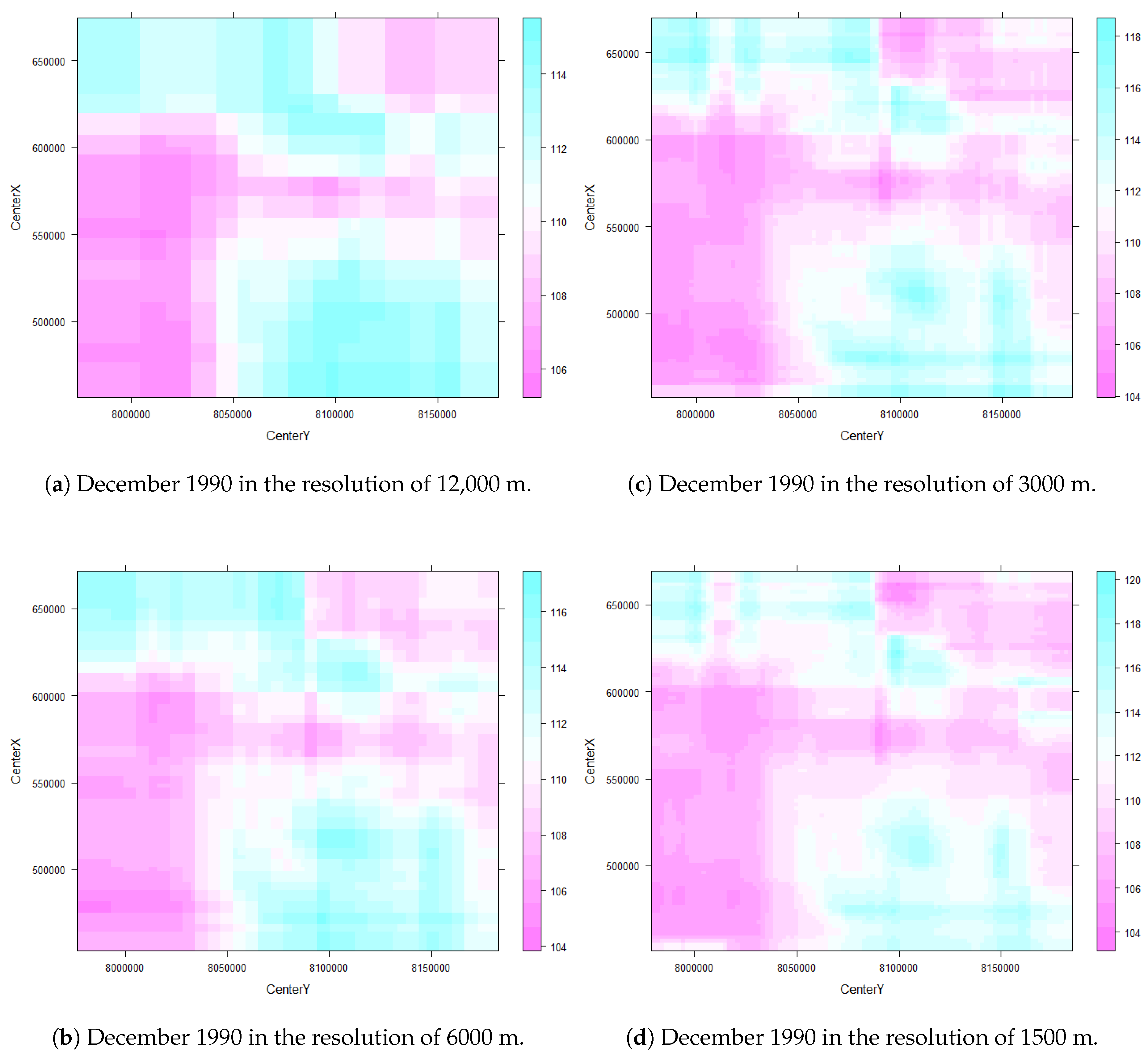
A spatial aggregation of remotely sensed data results generally in a loss of spatial detail. If the object of interest is, however, bigger than the pixel resolution an optimal resolution needs to be identified. In the case of monitoring heterogeneous land with Landsat (30 m pixels) a spatial aggregation and data reduction of remotely sensed information results in a smoothing effect and with increasing coarseness small features will become lost or mixed into neighbouring pixels. This is especially crucial when predicting green vegetation in different spatial aggregations resolutions where spectral information of green vegetation will be averaged over large areas. However, an increasing coarseness enables a faster processing time and is more efficient when dealing with big data challenges.
The Red and Near Infrared [
1] spectral information of remotely sensed imagery have considerable potential for monitoring green vegetation on a regional or local scale. Remote sensing measurement devices are not in direct contact with the objects they sense and therefore, offer great advantages and potential in recording large areas. Remotely sensed data are available from a wide range of sources, ranging from satellites to drones, and have been used for a very wide range of environmental applications [
2,
3,
4,
5,
6,
7,
8,
9,
10].
There is a strong advantage in using remotely sensed Landsat imagery for land use and land cover (LULC) analyses [
11,
12]. Landsat data are freely available [
13], the imagery covers a wide geographical area, and it avoids expensive, extensive and often impractical in situ measurement. The spatial resolution of a satellite pixel combines the reflected or emitted radiation from different objects on the Earth’s surface, and this spectral mixing effect results in a so-called mixed pixel [
14] or Mixel. With the decrease of spatial resolutions, spectra from individual objects cannot be separated and linked to specific features on the ground. There is a range of earth observation satellites available, with different spatial resolution, for example, MODIS (250, 500 and 1000 m) with a high temporal resolution to monitor vegetation health, Sentinel-2A/2B that simultaneously records land surface reflectance with a spatial resolution starting from 10 m up to 60 m, Sentinel 3 (Full resolution: 300 m and reduced resolution: 1.2 km) primarily used for climate-related studies on sea-land-surface temperatures, AVHRR (1.1 km) to monitor clouds and the thermal emission of terrestrial land, and SeaWiFS (1 km) that can quantify chlorophyll produced by marine phytoplankton. We refer to high resolution as <15 m, moderate resolution as 15–100 m, and low resolution as >100 m. LULC analysis using low spatial resolution (hundreds of meters) is more suitable for studies related to climate change, climate variability and environmental degradation.
Fractional cover (FCover) is a derived product based on Landsat 5 Thematic Mapper (TM) imagery. In a spectral unmixing approach the Landsat mixel information is separated into assigned biophysical variables, here bare soil, photosynthetic vegetation (green vegetation) and non-photosynthetic vegetation [
15,
16,
17,
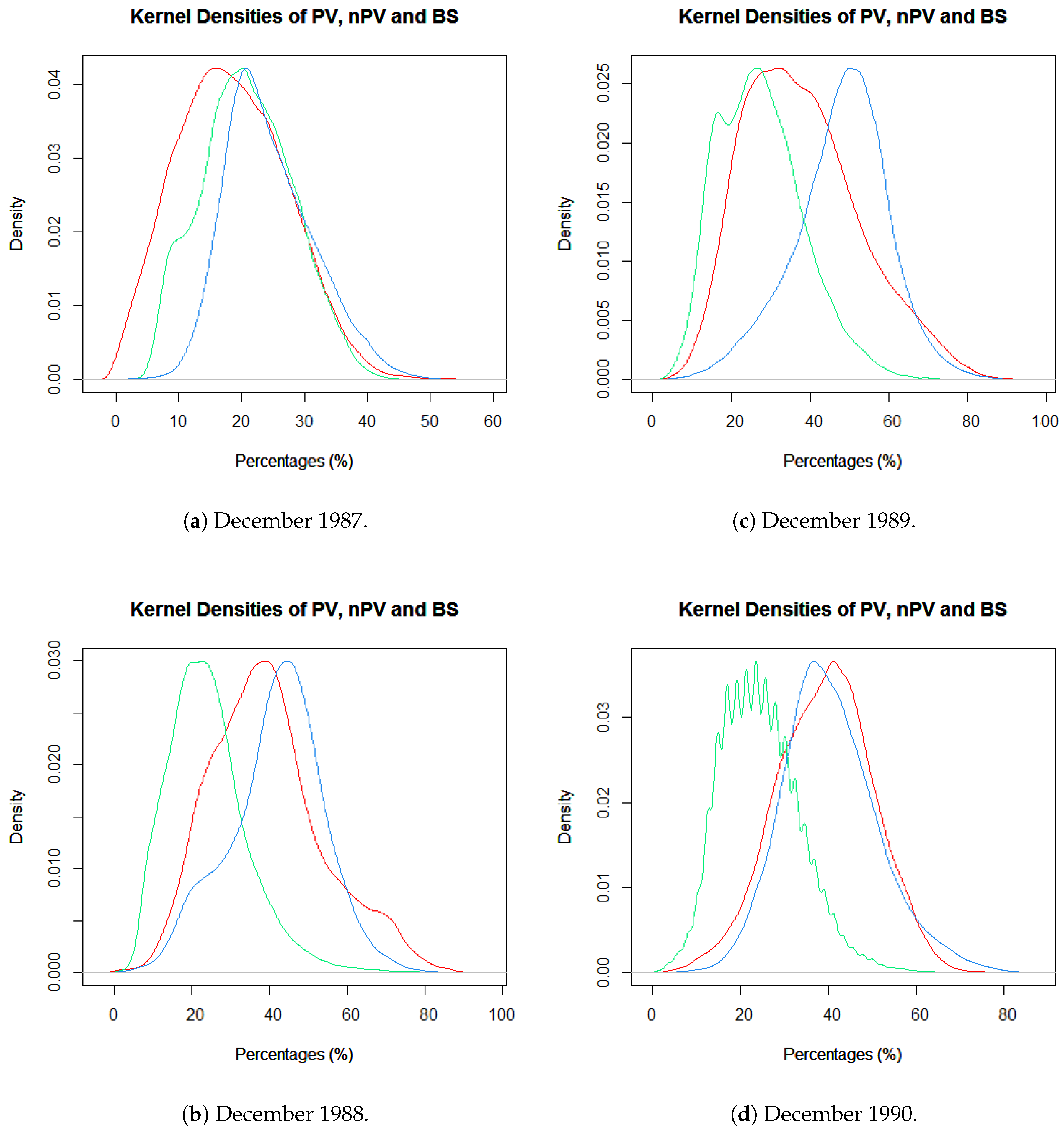
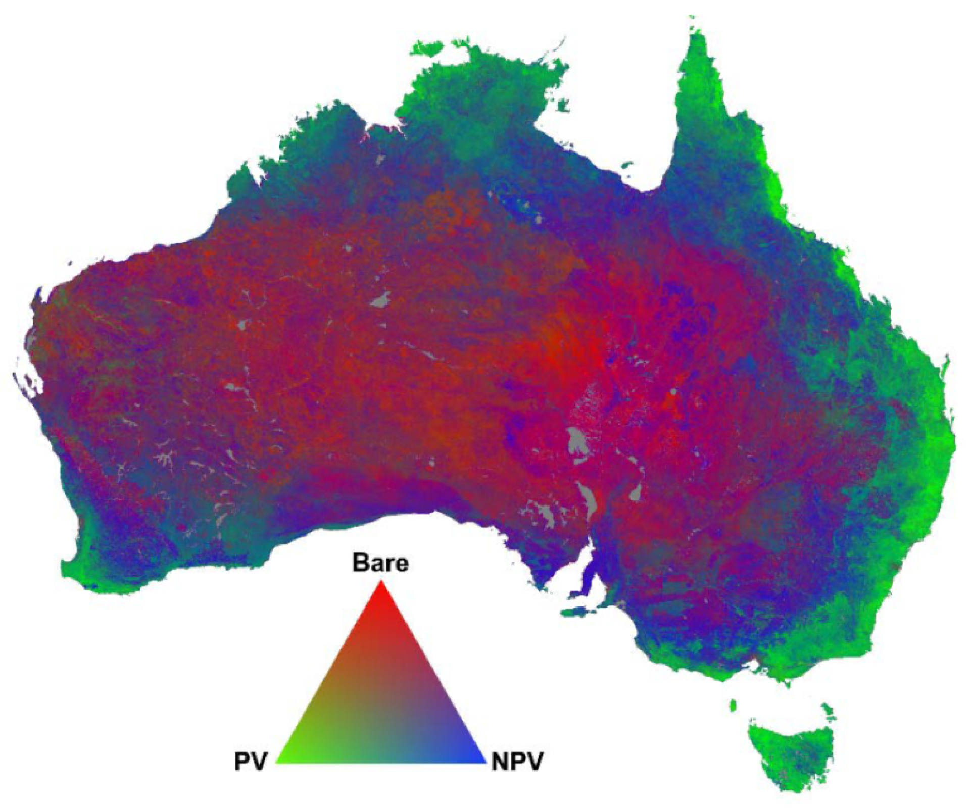
18]. A spectral unmixing technique was applied to estimate the proportion of green vegetation (PV), senescent or non-photosynthetic active vegetation (nPV) and bare soil (BS) represented in one pixel as percentages ranging from 0% (no representation of one ground cover type) to 100% (full representation) [
15,
18]. However, spectral unmixing is not limited to these fractions and not to Landsat imagery. The spectral unmixing approach used for our FCover data is described in [
15,
19,
20].
Using FCover provides a major advantage over using spectral bands and their derived vegetation indices like the NDVI. It is not required to perform an additional ground truth assessment since an extensive data collection has been conducted to collect samples of ground cover that are used for the spectral unmixing algorithm. The Australian FCover we are using for our case study is a standardised and validated product on similar LULC types on heterogeneous land and provided by a state government agency with an overall error of the fractional ground cover with an RMSE of 11.8% [
21]. A description of how the ground cover samples were collected is given in [
19].
FCover imagery is a fundamental site and landscape scale measurement required by landholders, non-government organizations and state and federal government departments in Australia [
22]. PV, nPV and BS are calculated using spectral unmixing models linked to an intensive field sampling program whereby more than 600 sites covering a wide variety of vegetation, soil and climate types were sampled to measure over-storey and ground cover [
23]. Fractional cover mapping has been applied in several rangeland systems [
24,
25,
26].
In Australia, FCover products are routinely produced using Landsat imagery and are available at the Terrestrial Ecosystem Research Network (TERN) AusCover remote sensing data archive [
22]. The AusCover Data portal aims to deliver consistent national time-series of remotely sensed biophysical parameters to support ecosystem research and natural resource management communities in Australia. These remote sensing products are based on past, current and future satellite image data sets with deliverables designed for Australian conditions. A similar and related product is persistent green vegetation fractions, that focus on woody and mostly vertical vegetation, such as trees, tree cover, tree density and canopy research [
21].
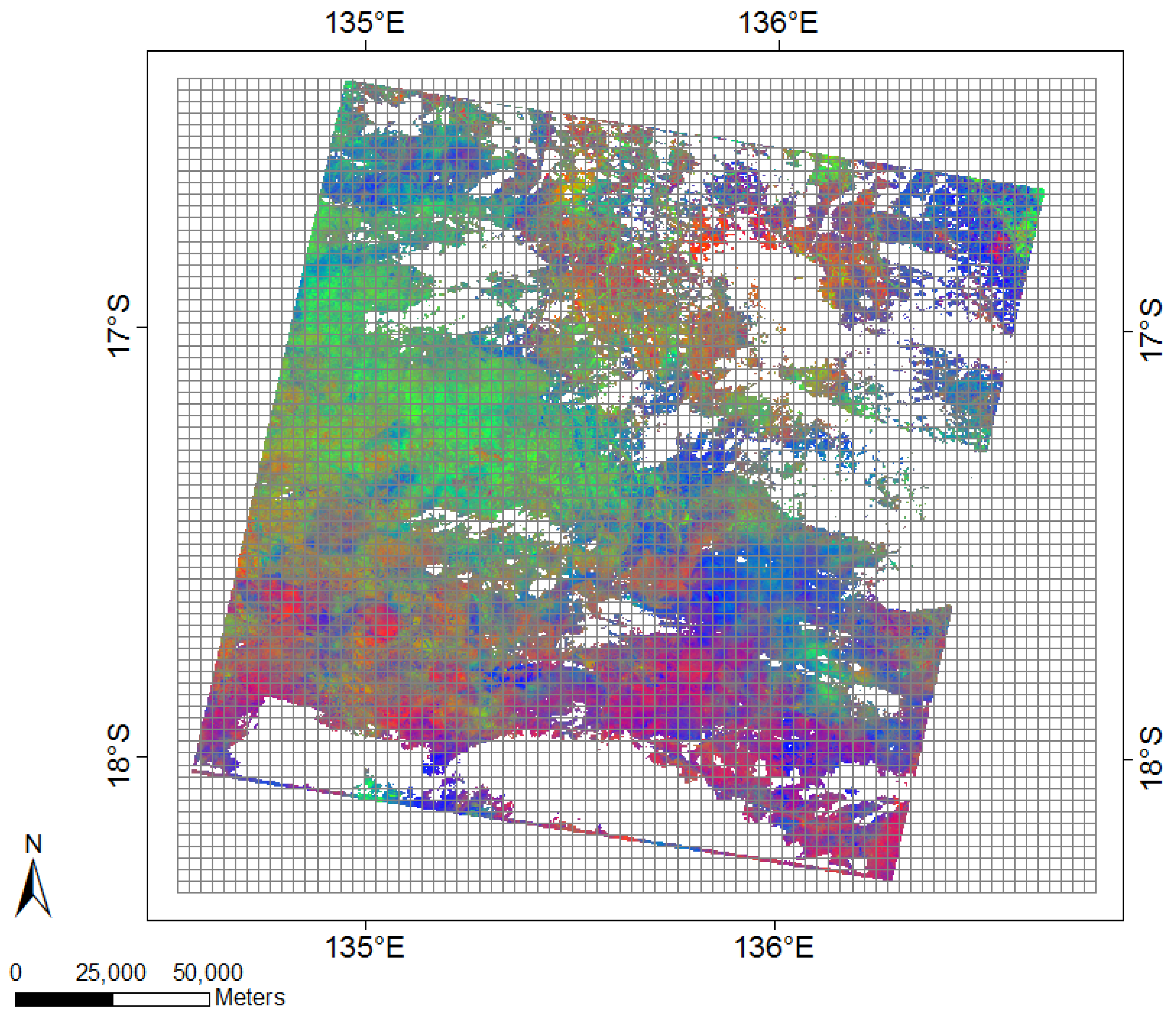
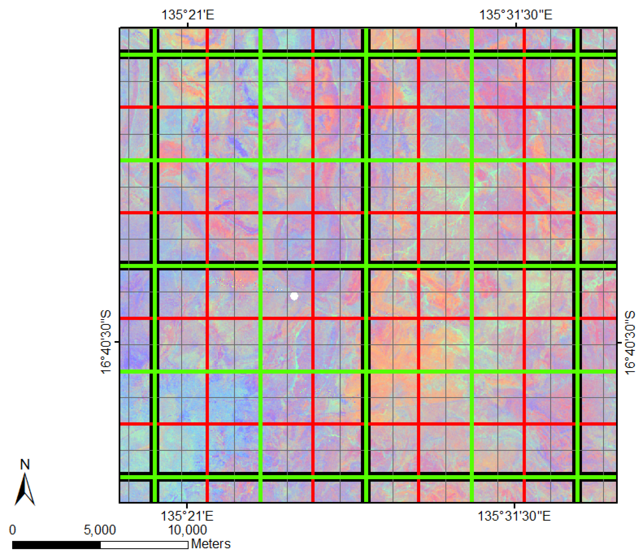
One way to reduce data volume is to aggregate pixels, but this is at the potential expense of loss of accuracy in assigning LULC types based on the coarser FCover values. In this paper, we investigate this issue by creating four even spaced grids and overlaying these on the FCover scenes. All pixels contained with the cell extent are then aggregated by calculating the arithmetic mean representing the green vegetation of this specific grid cell. This aggregation adds an additional level of uncertainty in the estimation of the coefficients of the model. However, by aggregating the fractions of green vegetation we create a source of potential bias and uncertainty in statistical analyses at different spatial resolutions. The modifiable area unit problem (MAUP) occurs when continuous measures of spatial phenomena are aggregated into a higher order grid [
27]. The association between variables depends on the size of the grid cell extent over which the FCover fractions are averaged.
Ershadi et al. [
28] investigated the effect of aggregating heat surface flux from fine (<100 m) to medium (approx 1 km) resolution using Landsat 5 imagery and indicated that aggregation using simple averaging methods have limited effect on land surface temperature compared to more sophisticated approaches. Moreover, by using the simple arithmetic mean to extract the required fraction of each grid cell we preserve the spatial distribution over the whole FCover scene [
29].
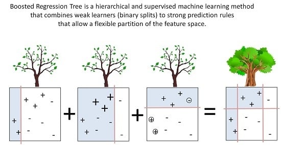
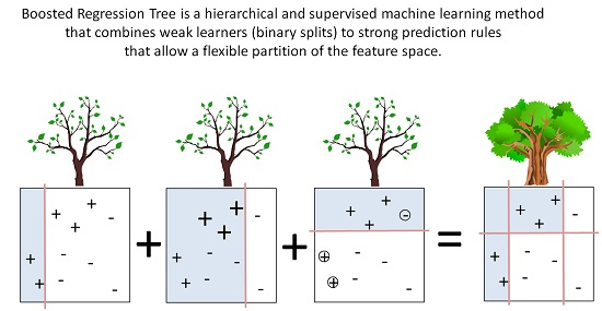
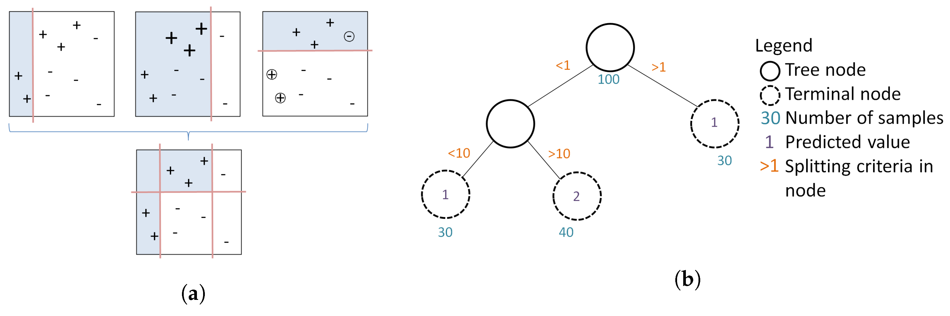
In this paper, we use a boosted regression tree (BRT) to link the response variable (FCover) to the two covariates, namely latitude and longitude of the centroid of the area. A BRT is a popular statistical and supervised machine learning approach that has been readily applied to remotely sensed data. Indeed, although they were first defined two decades ago, BRTs have only recently been extended to deal with the types of features that are characteristic of remotely sensed data, in particular, its spatial and temporal dynamics. BRTs combine two algorithms (regression trees and boosting) and arguably yield higher prediction accuracy than simple tree-based methods such as a Classification and Regression Trees (CART) [
30]. There are two major advantages of using BRT over more traditional regression methods. First, it allows a more flexible partition of the feature space that is not as rigid as using a simple linear regression. BRT combines simple binary partitions to form a complex prediction rule that can more accurately identify small areas of interest. Second, it can deal with missing values by default, such as masked out areas (clouds and cloud shadows), water bodies or the Scan Line Error of Landsat 7 ETM+. This is a great advantage especially when using remotely sensed imagery that has gone through several quality refinements and processing levels to filter out obscuring elements that leave data gaps behind.
The aggregated fractions of green vegetation derived from the FCover scene serve as our response variable. The delineated centroid coordinates from the midpoint of the spatial grid cells serve as surrogates for other spatial covariates and represent a north-south gradient shown as a vector of latitude coordinates and an east-west gradient shown as a vector of longitude coordinates. These surrogate variables will be used to statistically analyse the relationship to our response variable and the quantitative impact on prediction accuracy of different spatial aggregation schemes.
The use of latitude and longitude as surrogates for other covariates is not uncommon. For example, in a study of the geographic distribution of plant functional types [
31] the authors examined the relationship of precipitation and temperature on C3 and C4 grass types and shrubs using latitude and longitude coordinates and concluded that latitude and longitude can be used as surrogate variables for the main climatic dimensions in North America. The latitude and longitude explained a substantial portion of the variability of the distribution of the relative abundance of shrubs, C3 grasses, and C4 grasses. Along a given longitude, C3 grasses increased with latitude. As one moves westward, C4 grasses are replaced by shrubs. In another study [
32] the authors plotted latitude and longitude coordinates and included these as surrogate variables to account for variation in climate associated with geographic location within deciduous forested ecoregions. The response was an aggregated NDVI variable used as an on-site quantification of vegetation in North America.
In summary, the objective of our study was to analyse the statistical dependence between our two surrogates, the centroid coordinates in latitude and longitude, and their ability to predict the aggregated fractions of green vegetation delineated from the FCover scene. The focus is on the prediction accuracy achieved in four spatial resolutions and the preprocessing time needed to extract and aggregate the green fractions out of the FCover scene. We use a BRT to link FCover with the two covariates.
The paper is structured as follows.
Section 2 presents the data and BRT methodology used for predicting green vegetation using geographic centroid coordinates of evenly spaced spatial grid cells, the relevance of the spatial aggregation measured as a model fit and a brief reminder about the principles of spectral unmixing approaches and its outcome.
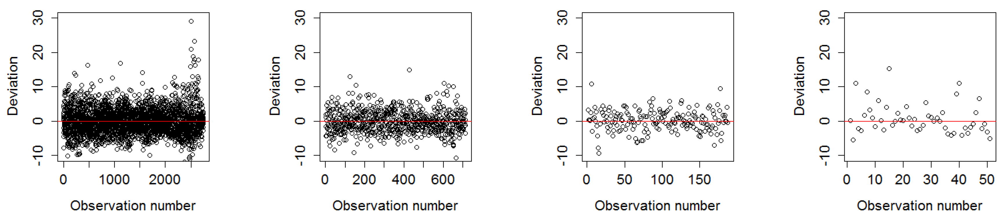
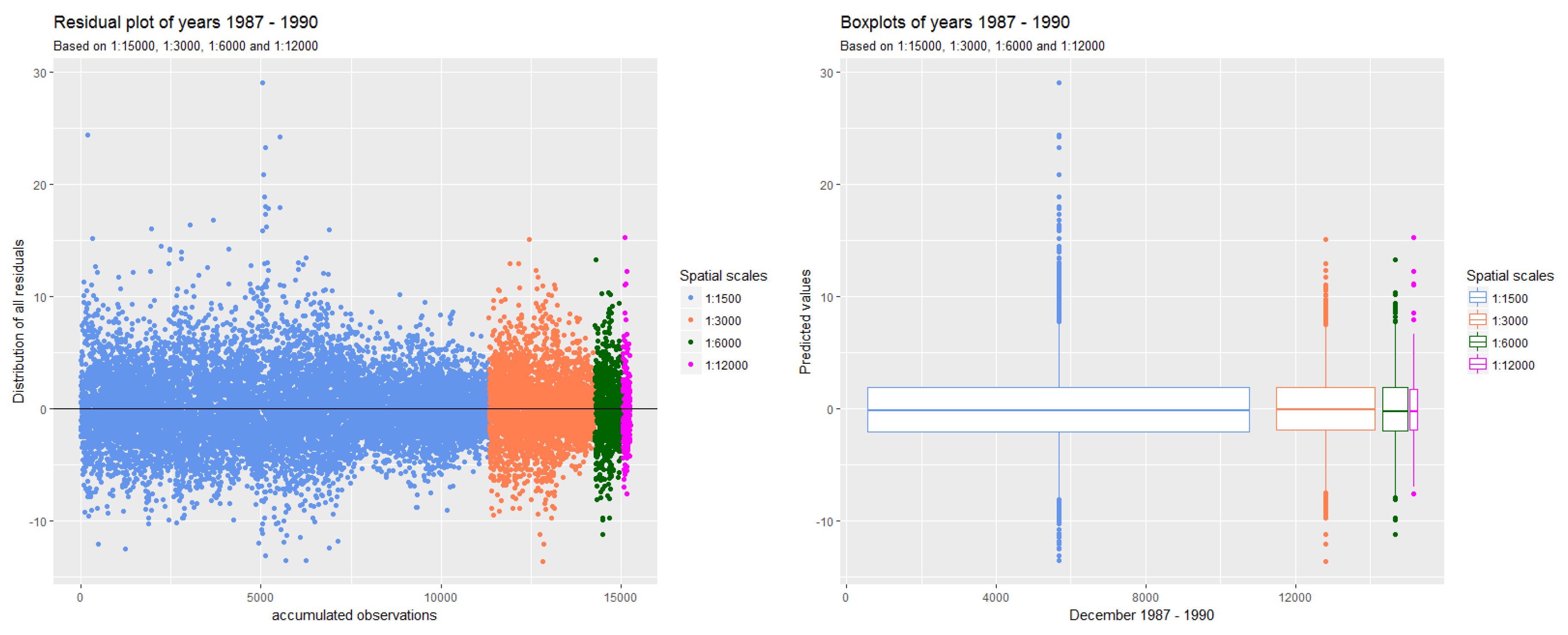
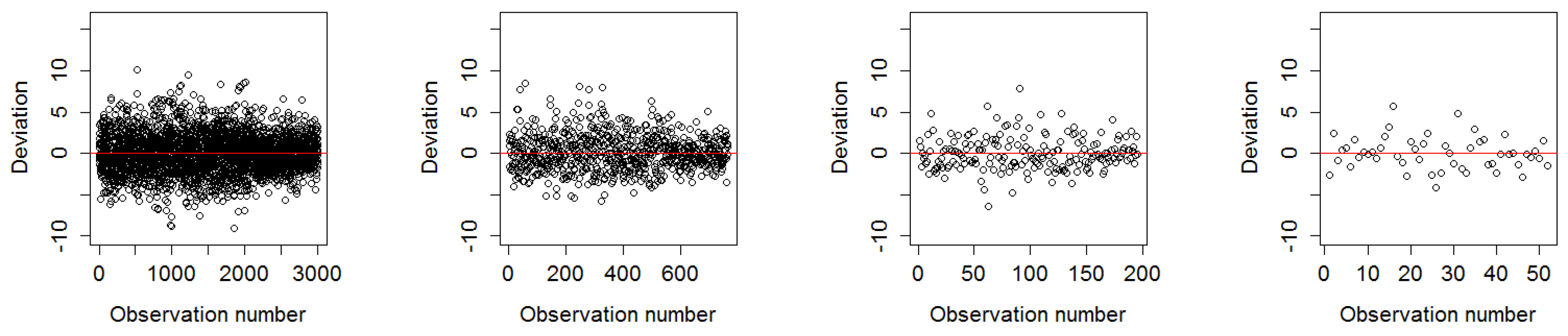
Section 3 presents the results structured in three groups: (1) the comparison of the model fit showing the distribution of the residuals around the mean, (2) the variable interactions as the relative influence and partial dependencies of the covariates on the response variable, the relationship and distribution of the predicted versus the observed test data set in marginal plots and model diagnostics and (3) the aggregation and scaling errors using different spatial resolutions. The outcome and the relevance of this work to real word scenarios and limitations of BRT are discussed in
Section 4.
4. Discussion
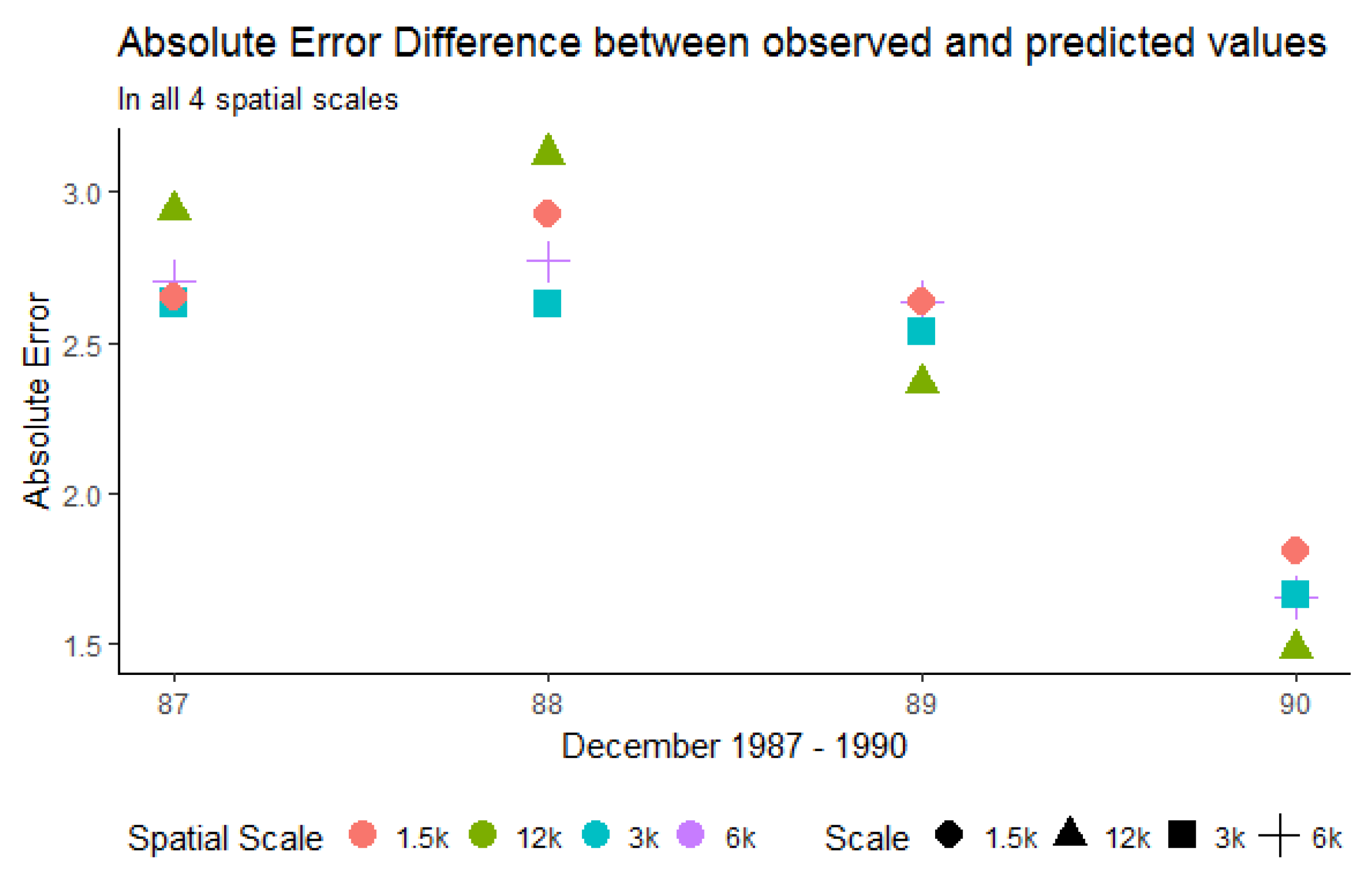
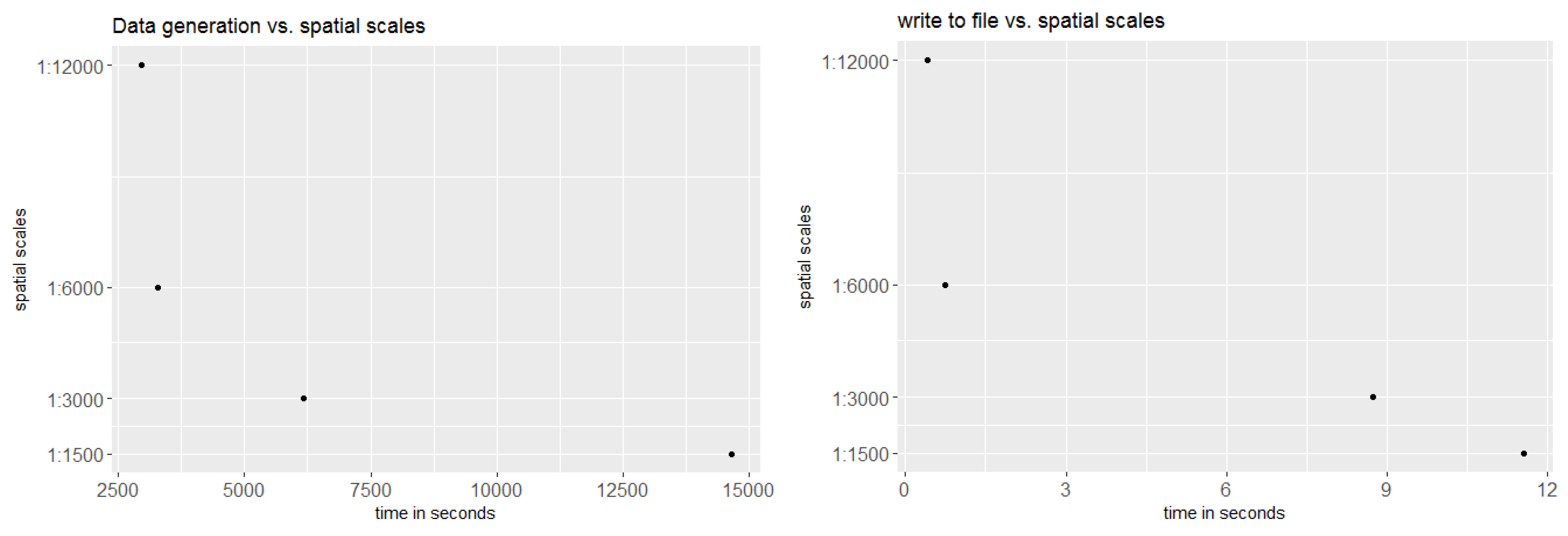
The goal of this paper was to investigate how spatial aggregation affects prediction accuracy of green vegetation using a BRT model. We focused our evaluation on a case study and chose four aggregation schemes that follow a linear scale. Aggregating the fractions of green vegetation and calculating the mean does alter the original fractions of PV. This alteration can be seen as the consequence of data compression. In our case, we introduced a compression that causes loss since the original fractions cannot be recovered by decompression. The results show that it is not necessary to compute FCover at full (30 m) spatial resolution to obtain satisfactory predictions. This is an important outcome since the computational time will be significantly reduced by spatially aggregating the fractions of the FCover scene.
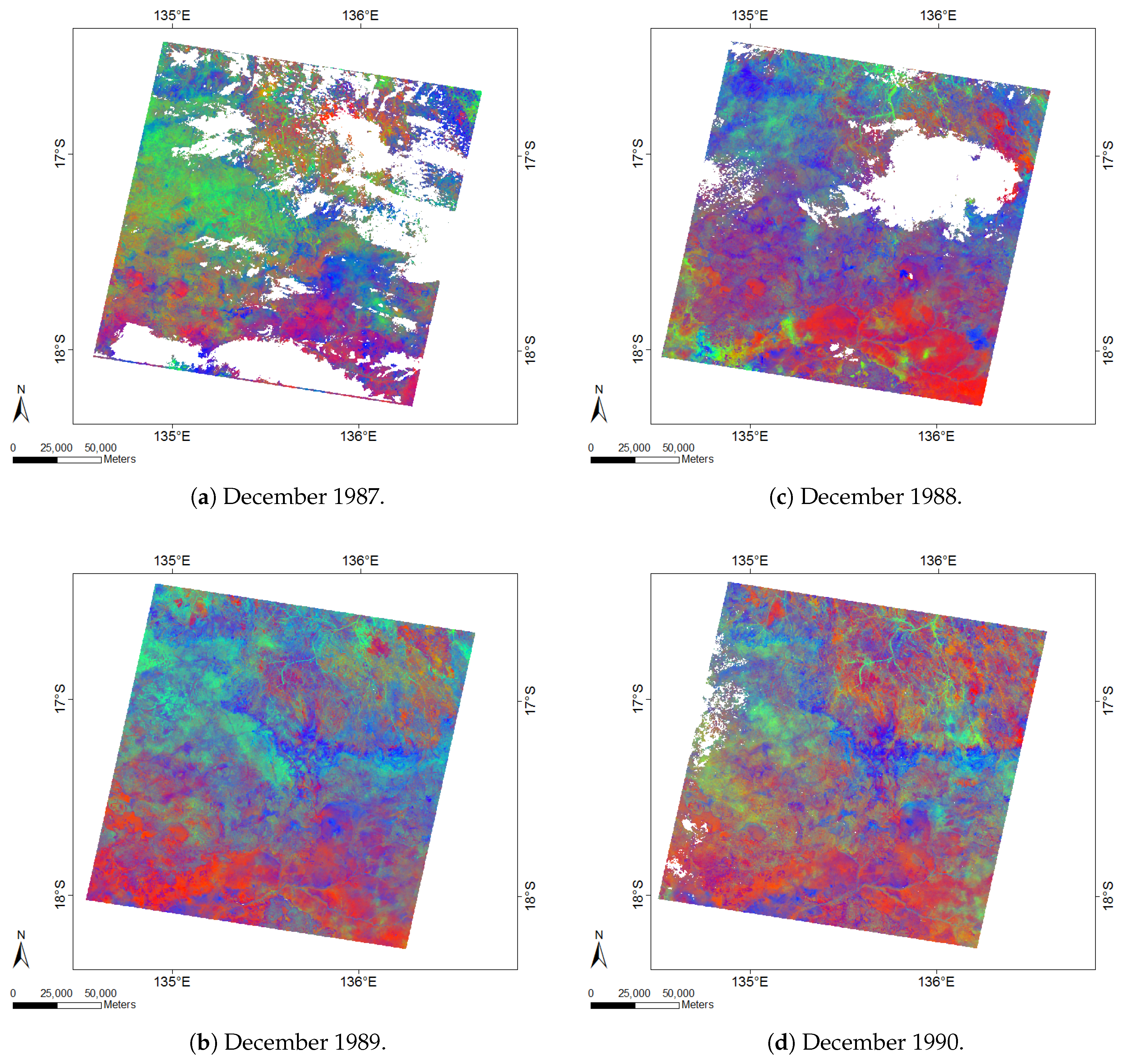
Figure 16 shows the reduction of time needed for the data generation process in extracting the means. This is especially important when more than one FCover scene is used. However, comparisons between aggregations are not straightforward, particularly because the data quality (showing large data gaps) and green vegetation cover differs between the scenes. Further investigation is still necessary to test BRT on homogeneous land to assess whether the best spatial aggregation resolution identified here as 6000 m is still the same and whether the prediction accuracy is affected by a different topography. We demonstrated that the BRT outperformed the LM by achieving much better RMSE rates.
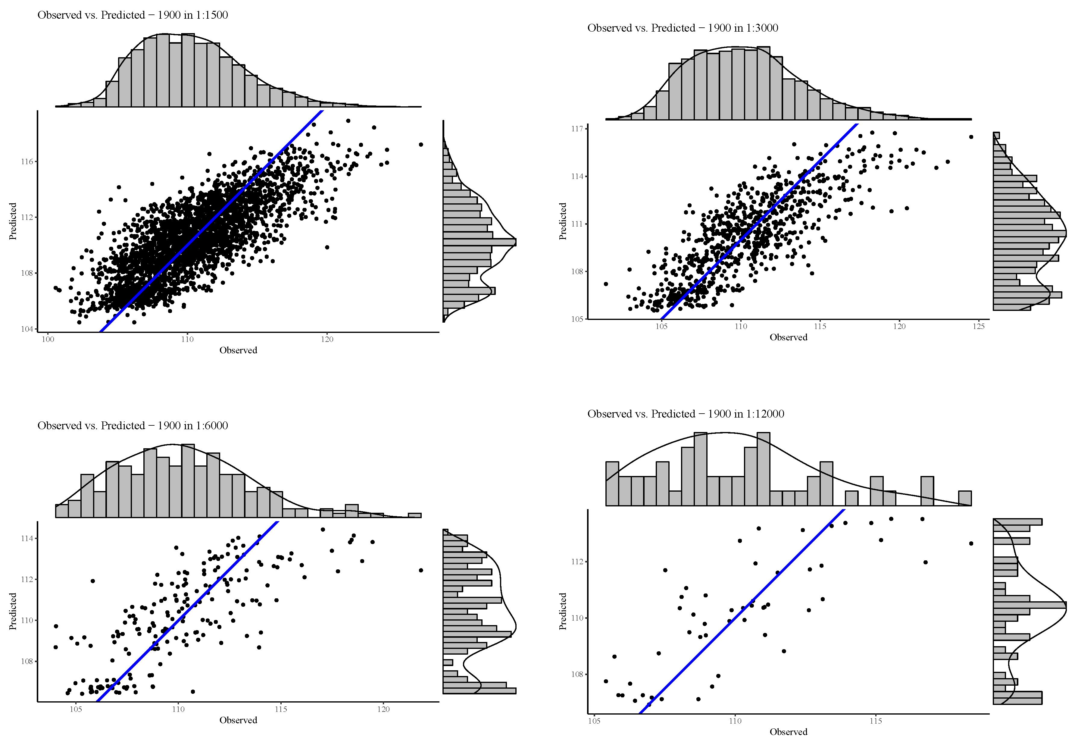
In this paper, we first demonstrated that the distribution of residuals around the mean is relatively consistent throughout the resolutions. Moreover, in our study latitude and longitude coordinates alone were shown to be able to effectively predict FCover. We showed the strong relationship between latitude and longitude in the marginal plots in
Figure 15.
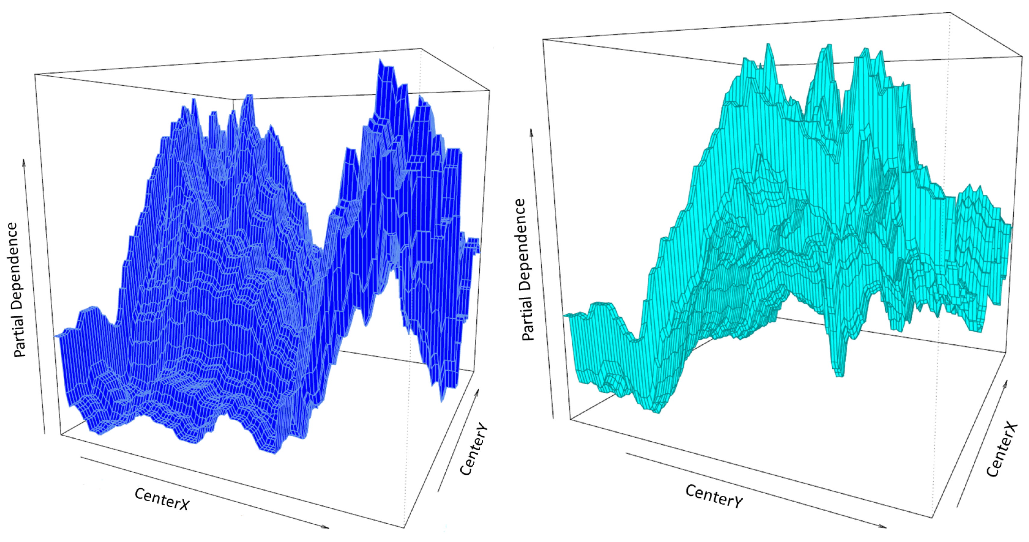
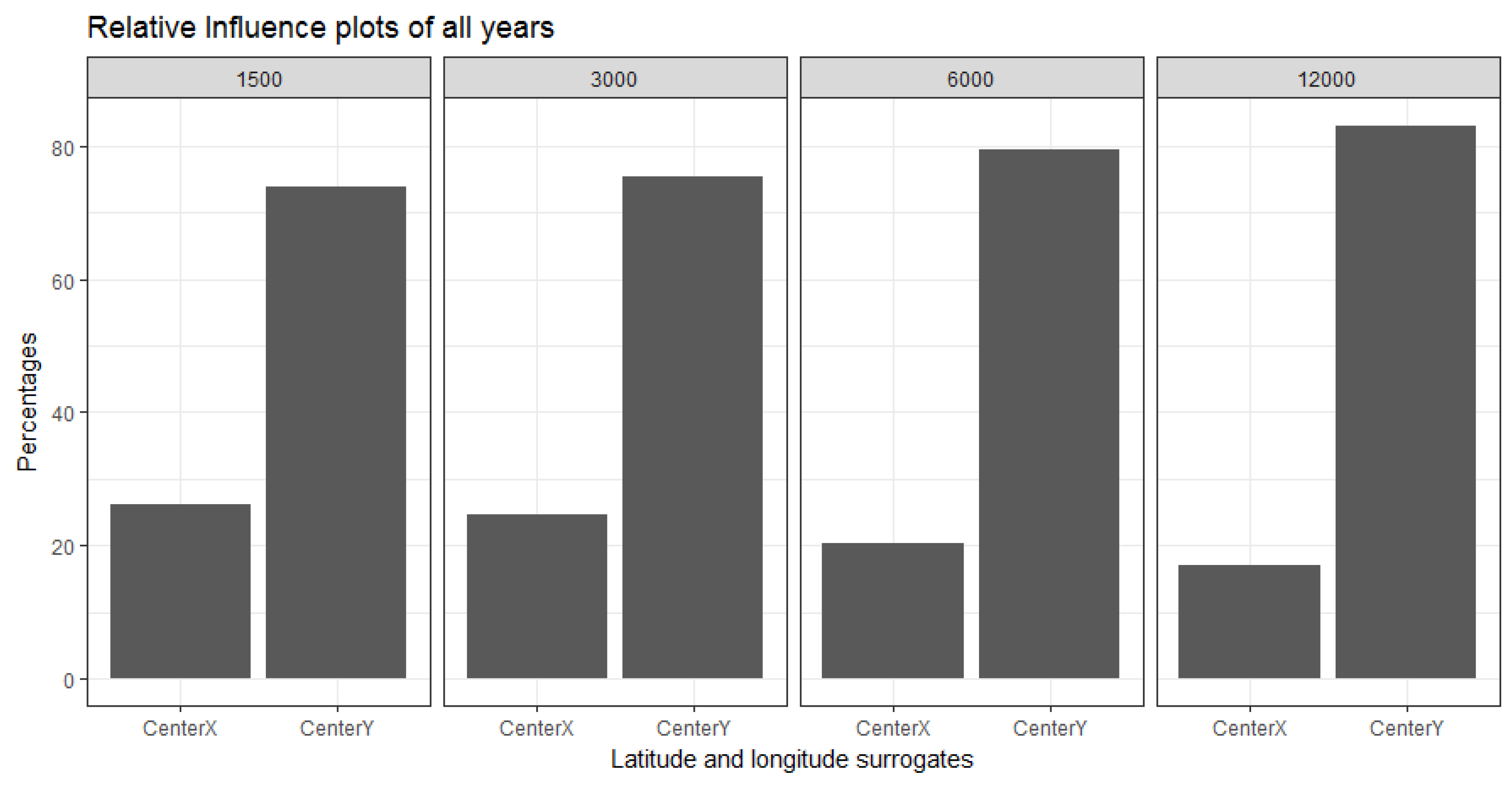
In the relative influence plots we demonstrated that the centroid of the latitudes (indicating North-South direction) are far more dominant in describing the aggregated FCover mean values. For reasons discussed in
Section 2.2 it is not surprising that the latitude dominates over longitude with regard to green vegetation. What is surprising though is the high contribution and very strong influence of around 80% as shown in
Figure 12.
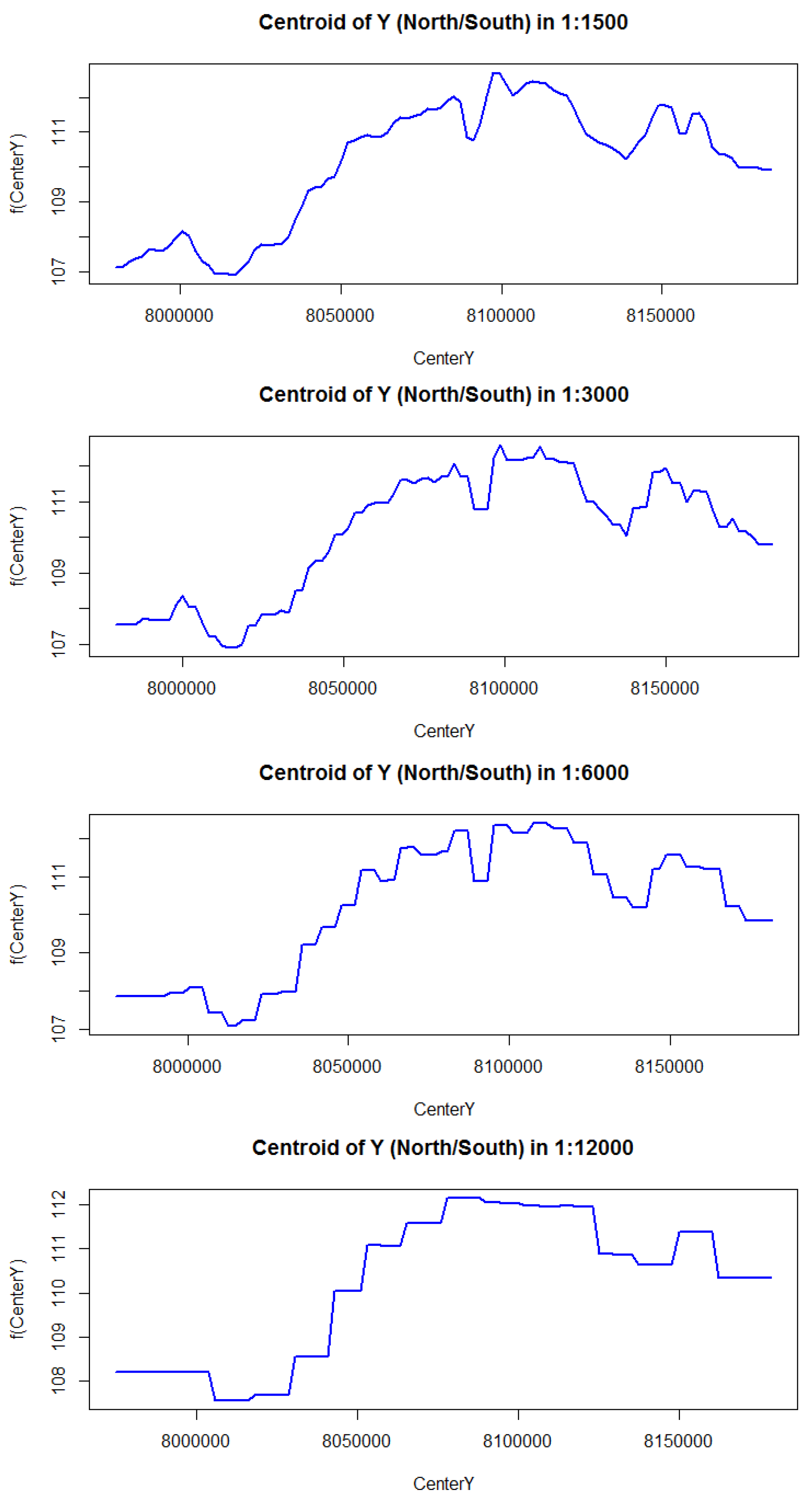
The marginal plots illustrate that BRT under-predicts high peak values throughout all resolutions. We argue that 72 FCover mean values of 12,000 m can represent the existing green vegetation in one scene. Further, we could demonstrate that the scene offered enough heterogeneous land cover and the Landsat footprint of 185 × 185 km was sufficient to show the targeted and generalisable results.
Another interesting investigation would be to use multi-sensory imagery and multi-granularity pixel sizes as additional covariates in the modelling process. We focused on the exact alignment of pixel edges to the spatial grid by choosing a resolution that incorporates full pixels. However, before we used the resolutions here, we had more common ones in 1000 m, 5000 m and 10,000 m and the data extraction time was significantly increased due to the effect of incorporating adjacent pixels that overlapped with the spatial grid cell.
Limitations of our approach can be found in the aggregation scheme using the arithmetic mean. When extracting the mean of a spatial grid cell we do not know the distribution of fractions within the grid cell since we only obtain one value representing the aggregated fractions. Different methods of aggregating values may provide better capture of cell statistics and data structure within a spatial grid cell.
An alternative way of using FCover fractions is to sum all the vegetation (nVP and VP) and compare those values with the fraction of bare soil in a presence/absence study. This could be useful in time series analysis, such as an investigation of an increase or decrease of vegetation versus bare soil. This is of particular interest with ongoing climate change towards desertification in arid or semi-arid areas. A potential approach is to use indicator functions that can encode logical and simple calculations by defining thresholds in order to investigate if fractions of the combined vegetation versus bare soil represent values greater than the set threshold of both classes. Depending on the magnitude of a fraction, the pixel could be mapped to categorical values used in the modelling process instead of our approach of using continuous values. BRT can deal with continuous and categorical response values.
There are many features of BRT that are advantageous for the problem considered here. The BRT model itself comprises a flexible regression structure with improved predictive performance effected through boosting. Boosting is an adaptive method for combining many simple models to give an improved predictive performance. In addition to the computational speed and accuracy of estimation, they can describe complex non-linearities and interactions between variables, accommodate missing data, include different types of input variables without the need for transformations or elimination of outliers, perform well in high-dimensional problems, and allow for different loss functions such as accurate identification of small areas of interest. Moreover, they can be visualised and interpreted easily, thus facilitating the translation of the analytic results to decision makers [
44]. The predictive accuracy of BRT has been investigated both theoretically [
42,
43] and in various applications [
51]. Although BRT models are complex, they can be summarized in ways that give powerful ecological insight, and their predictive performance is superior to most traditional modelling methods.
To sum up, BRT is a very flexible, statistical and hierarchical machine learning approach that can be used in various remote sensing aspects. In a study by Kotta [
52] the author combined hyperspectral remote sensing and BRT to test their ability to predict macrophyte and invertebrate species cover in the optically complex seawater of the Baltic Sea and concluded that there is a strong potential for BRT in modelling aquatic species. Further, Jafari et al. [
5] evaluated the suitability and performance of BRT for soil mapping using a limited point dataset in an arid region of Iran. The performance was tested in two scenarios: (i) using only the DEM and remote sensing covariates and (ii) additionally using the geomorphology map. Results showed that the geomorphology map contributed importantly to the prediction accuracy. In addition, Colin et al. [
50] combined a collection of GIS shapefiles, remotely sensed imagery, and aggregated and interpolated spatio-temporal information to one input file that resulted in a structured but noisy input file, showing inconsistencies and redundancies. It was shown that BRT can process different data granularities, heterogeneous data and missingness. A comparison with two similar regression models (Random Forests and Least Absolute Shrinkage and Selection Operator, LASSO) showed that BRT outperforms these in this instance. Last but not least, Pittman [
53] investigated coral reef ecosystems that are topographically complex environments and possess structural heterogeneity that influences the distribution, abundance and behaviour of marine organisms. They used BRT and LIDAR data that provided high resolution digital bathymetry from which the topographic complexity was quantified at seven spatial resolutions of 4, 15, 25, 50, 100, 200 and 300 m [
53]. They concluded that the combination of BRT and LIDAR has a great utility in the future development of benthic habitat maps and faunal distribution maps to support ecosystem-based management and marine spatial planning.

 ,
, 


