Abstract
Information on the spatial distribution of forest structure parameters (e.g., aboveground biomass, vegetation height) are crucial for assessing terrestrial carbon stocks and emissions. In this study, we sought to assess the potential and merit of multi-temporal dual-polarised L-band observations for vegetation height estimation in tropical deciduous and evergreen forests of Mexico. We estimated vegetation height using dual-polarised L-band observations and a machine learning approach. We used airborne LiDAR-based vegetation height for model training and for result validation. We split LiDAR-based vegetation height into training and test data using two different approaches, i.e., considering and ignoring spatial autocorrelation between training and test data. Our results indicate that ignoring spatial autocorrelation leads to an overoptimistic model’s predictive performance. Accordingly, a spatial splitting of the reference data should be preferred in order to provide realistic retrieval accuracies. Moreover, the model’s predictive performance increases with an increasing number of spatial predictors and training samples, but saturates at a specific level (i.e., at 12 dual-polarised L-band backscatter measurements and at around 20% of all training samples). In consideration of spatial autocorrelation between training and test data, we determined an optimal number of L-band observations and training samples as a trade-off between retrieval accuracy and data collection effort. In summary, our study demonstrates the merit of multi-temporal ScanSAR L-band observations for estimation of vegetation height at a larger scale and provides a workflow for robust predictions of this parameter.
1. Introduction
The status of tropical forests and their temporal dynamics can be assessed and monitored by measuring different forest biophysical parameters (e.g., vegetation height, canopy cover, stem volume and aboveground biomass (AGB)). Accurate spatial estimates of these parameters are crucial to assess terrestrial carbon (C) stocks and C-emissions, as well as to develop sustainable forest management strategies. Furthermore, these products can help provide a better understanding of the ecosystem dynamics and the effects of environmental drivers through modelling. Field measurements of forest biophysical parameters are, however, associated with high costs (e.g., they are labour intensive and time consuming) and are limited to point measurements, which may not adequately describe patterns at different spatial scales. Spatially explicit information on three-dimensional vegetation structure can be provided by Light Detection and Ranging (LiDAR) sensors (e.g., [1,2,3]). Laser pulses sent from a sensor are capable to penetrate the forest canopy and to directly measure vertical vegetation structure. LiDAR is usually operated from an airborne platform and thus limited to small spatial coverage. Both spaceborne as well as airborne LiDAR may provide samples of forest structure parameters over large areas (e.g., regional, national, continental scales) and need to be integrated with satellite imagery to derive wall-to-wall estimates of forest biophysical parameters.
Satellite imagery collected by Radio Detection and Ranging (RADAR) sensors are sensitive to forest structure parameters (e.g., [4,5,6,7,8,9,10,11]), as microwave signals have the capability to penetrate the vegetation profile, and thus to probe the three-dimensional vegetation structure. Furthermore, RADAR data are particularly useful for weather independent applications, as long wavelengths (with a spectral range between 1 cm and 1 m) penetrate clouds. A key parameter obtained from Synthetic Aperture Radar (SAR) data, backscatter intensity, measures the return energy from a target and is determined by the geometric and dielectric properties (which is mostly determined by the water content) of the reflective material, as well as by the frequency, polarisation and angle of incidence of the emitted wave [12]. Long wavelengths (e.g., at P-band and L-band) are more suitable for the retrieval of forest structure parameters (e.g., growing stock volume, AGB) because of their ability to penetrate deeper in forest canopies as compared to short wavelengths (e.g., at X-band and C-band) [7,13,14], and thus to interact with large branches (in order of the wavelength) and trunks. In general, the cross-polarised (HV, VH) waves are induced by volume scattering [15] (e.g., as occurring within woody canopies) and are thus more sensitive to volume and possess a stronger correlation with forest structure parameters compared to co-polarised (HH, VV) waves [16,17]. Advanced SAR techniques (e.g., interferometry (InSAR), polarimetry (PolSAR), polarimetric interferometry (PolInSAR), tomography (TomoSAR)) show promising results for estimating vegetation structure parameters [18,19,20,21,22,23]. For instance, studies based on TanDEM-X single-pass interferometer (e.g., [18,19,24,25]) reported promising sensitivity of the InSAR height to canopy height and thus to stem volume and AGB in boreal and tropical forests. Since the temporal baseline of the TanDEM-X mission is quasi zero, temporal decorrelation of the interferometric coherence can be excluded, and the InSAR coherence is primarily impacted by volume decorrelation. Furthermore, due to the short wavelength of TanDEM-X data (i.e., X-band), most of the incoming electromagnetic energy is scattered from the top of vegetation and the TanDEM-X InSAR height exhibits a strong correlation with vegetation height. For PolInSAR analysis, at least two full polarimetric (i.e., all polarisations are available) SAR datasets acquired from two slightly different positions are needed to determine the volume phase scattering centre, which is located close to the top of a canopy. Accordingly, this measurement is useful to estimate tree height. For TomoSAR methods, a stack of multi-baseline SAR data is required to delineate SAR Tomograms. From the Tomogram, the 3D position and scattering amplitude of each relevant scatterer can be derived, i.e., individual tomographic layers can be classified as surface layers, topmost layers and volume layers (e.g., middle heights). However, currently only one of these methods can be applied for large-scale mapping (i.e., single-pass InSAR), due to the lack of PolInSAR and TomoSAR data at this scale. Moreover, single-pass interferometry based on TanDEM-X data is also somehow limited due to data policy, including restricted data access for scientific use. Because of the data availability and technically less complex analysis compared to InSAR, PolInSAR and TomoSAR, most studies on the estimation of forest structure parameters are based on SAR backscatter analysis (e.g., for AGB estimation [26]). For instance, L-band backscatter was successfully applied to map fractional woody cover [27,28,29,30,31] as well as regional or global forests [32,33,34,35]. Moreover, L-band backscatter was used to predict vegetation height in various biomes from boreal [36] and temperate [4,37,38] to tropical forests [39].
In this study, we examine the potential of multi-temporal L-band SAR backscatter acquired by the Advanced Land Observation Satellite 2 Phased Array L-band Synthetic Aperture Radar 2 (ALOS-2 PALSAR-2) in ScanSAR mode to estimate vegetation height over tropical deciduous and evergreen forests in the Yucatan peninsula, Mexico. ScanSAR data exhibit much larger swath width compared to Stripmap data (i.e., 350 km vs. 70 km) and accordingly can cover wider areas at higher repetition rates. For instance, ScanSAR acquisitions cover the entire tropical region approximately every 42 days. Therefore, we analyse the performance of the multi-temporal combination of L-band backscatter for vegetation height mapping. Airborne LiDAR-based vegetation height is used as reference data for model training and validation.
In this paper, we demonstrate the value of multi-temporal PALSAR-2 ScanSAR mosaics compared to open global PALSAR-2 Stripmap Fine Beam Dual Polarisation (FBD) mosaics. Moreover, we apply two different validation approaches to show the effect of spatial autocorrelation on model performance. In previous studies (e.g., [38,39]) it was reported that statistical models improve by increasing the number of spatial predictors as well as response variables. We examine these findings considering two different validation schemes, which include and minimise the autocorrelation. The results of the study are relevant in the context of the upcoming L-band missions for global vegetation monitoring (e.g., ALOS-4, NISAR, SAOCOM, Tandem-L) and an increasing number of L-band SAR data in the near future. Since vegetation height correlates with other forest parameters (e.g., AGB, tree canopy cover) [40,41,42], we can assume that similar results can be achieved for the estimation of AGB and tree canopy cover using multi-temporal dual-polarised L-band SAR backscatter.
2. Materials and Methods
2.1. Study Area
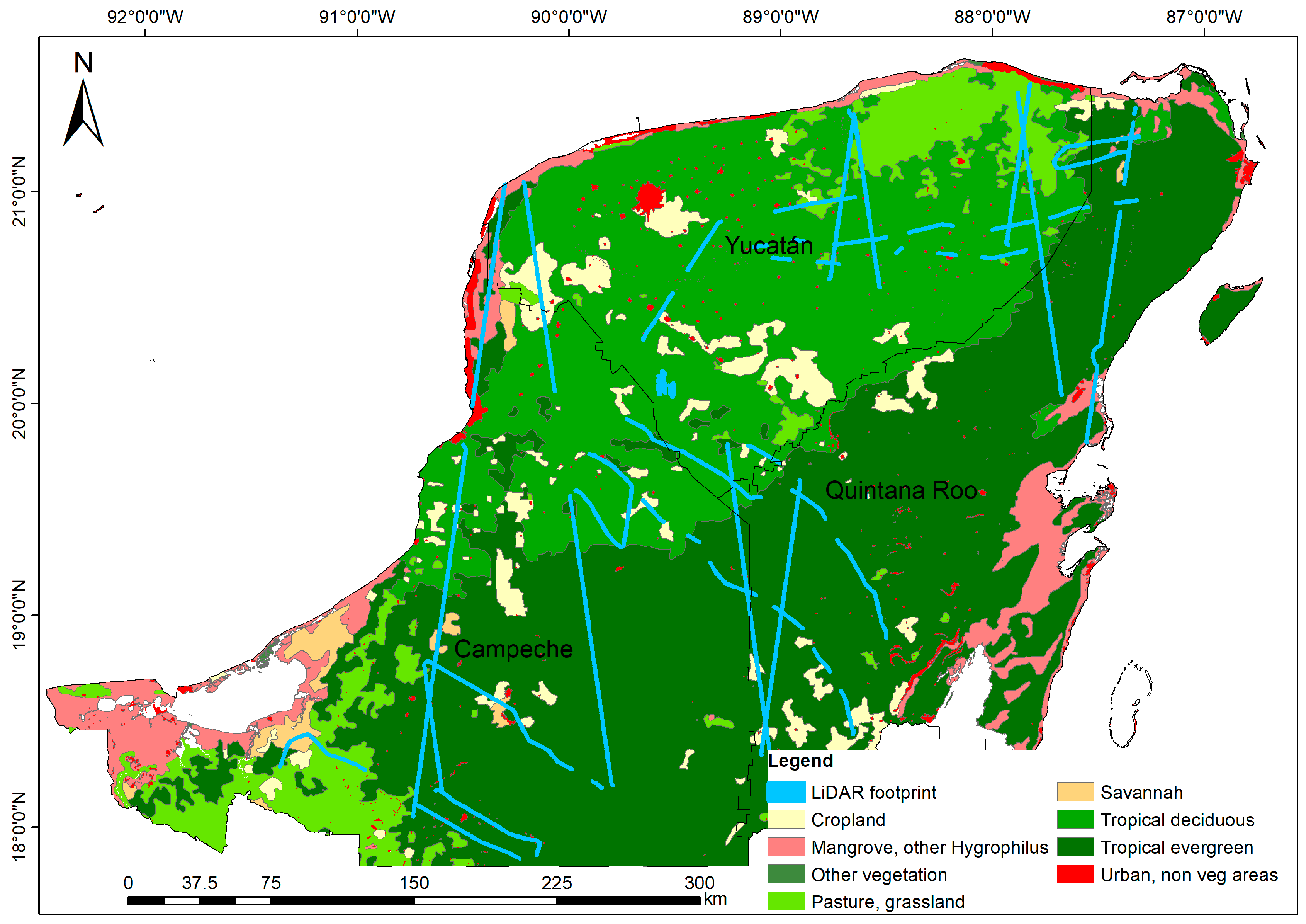
The study area is the Yucatan peninsula, Mexico, which is mostly covered by tropical deciduous and evergreen forests (Figure 1). According to a land use map for 2010 generated by the Mexican National Institute for Statistics and Geography (INEGI) [43], around 1/3 of the total area (i.e., ~140,000 km2) is covered by tropical deciduous forests (i.e., ~42,000 km2), whereas around 1/2 of the total area is covered by tropical evergreen forests (~68,000 km2). Based on ca. 5000 field plots collected over the entire peninsula during the National Forest Inventory programme between 2004 and 2011 [44], mean tree height is 9 m (max. height 27 m), mean diameter at breast height (DBH) is 13 cm (max. DBH 46 cm), mean basal area is 12 m2·ha−1 (max. 36 m2·ha−1) and mean AGB is 70 t·ha−1 (max. AGB 227 t·ha−1). The area of the peninsula is rather flat. According to the Shuttle Radar Topography Mission (SRTM) Digital Elevation Model (DEM) version 4.1 [45], average elevation is 62 m with a standard deviation of 70.8 m. The average slope is 1.3° with a standard deviation of 1.5°.

Figure 1.
Study area. Land use and vegetation map of Mexico from the Mexican National Institute for Statistics and Geography (INEGI) Series IV [43] with the available airborne LiDAR strips.
The regional climate is tropical sub-humid with slightly higher air temperatures in summer than in winter (Figure 2). The average annual temperature between 2013 and 2017 was ~27 °C [46]. Average annual precipitation ranges from 1000 to 1500 mm, while the period between May and November is characterised by pronounced rainfall, and the relatively dry period extends between December and April (Figure 2) [46]. Furthermore, the rainfall increases from north (~1100 mm mean annual total precipitation between 2013 and 2017 for the federal state of Yucatan) to south (~1400–1450 mm mean annual total precipitation between 2013 and 2017 for the federal states of Campeche and Quintana Roo, respectively). The forests in the north-western part of the peninsula have experienced slash-and-burn agriculture for 2000 years, resulting in forest patches at different succession stages [47]. In contrast, the southern and eastern parts of the Yucatan peninsula show one of the lowest annual deforestation rates, with some nearly intact areas of tropical forest in Central America (e.g., Calakmul Biosphere Reserve) [47].
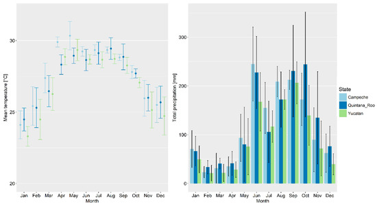
Figure 2.
Mean monthly air temperature (circles on the left-hand side) and total monthly precipitation (bars on the right-hand side) for three Mexican federal states for the years 2013–2017. Error bars represent monthly standard deviations.
2.2. Remote Sensing Data
2.2.1. Airborne LiDAR Data
Small-footprint discrete-return airborne LiDAR data were collected by the NASA’s G-LiHT imager [48] in April–May 2013 over entire Mexico (Figure 1). The average pulse density was approximately 6 returns·m−2. The data over the Yucatan peninsula were acquired during leaf-off conditions, which can lead to an underestimation of vegetation height. The LiDAR returns were classified into “ground returns”, “shrub returns” (i.e., non-ground returns below 1.37 m) and “tree returns” (i.e., returns above 1.37 m). From the topography-normalised point clouds, 88 plot-aggregated LiDAR metrics (e.g., percentiles, density metrics for “shrub returns”, “tree returns” and “all returns”) as described in [49,50,51] were calculated at 13 m spatial resolution. These LiDAR metrics correspond to the vertical structure of a target. Both LiDAR point cloud, as well as metrics, can be downloaded from the NASA G-LiHT data portal [52]. In this study, a LiDAR metric, percentile 100% of all returns (hereafter p100) (i.e., top-of-canopy estimate), was used as reference data (i.e., for model training and result validation). In the next step, we aggregated this LiDAR metric from 13 m × 13 m to 100 m × 100 m using block averaging and nearest neighbour resampling, i.e., a top-of-canopy estimate for a 13 m × 13 m pixel was averaged to 100 m. In total, ca. 150,000·1 ha LiDAR samples (ca. 1% of the total area of the Yucatan peninsula) were used as reference data for wall-to-wall mapping of vegetation height. Although LiDAR provides an estimation of height, its accuracy might be higher than field height measurements, especially in a forest with a closed canopy, where the top of a tree is difficult to detect from the ground.
2.2.2. SAR Data
The multi-temporal L-band SAR backscatter measurements used in this study were collected by the ALOS-2 PALSAR-2 sensor in dual-polarisation (i.e., HH and HV) ScanSAR mode between October 2014 and February 2018 (resulting in 24 ScanSAR mosaics). ALOS-2 PALSAR-2 ScanSAR data feature a swath width of ca. 350 km and a repetition rate of ca. 42 days [53]. The data were distributed by the Japan Aerospace Exploration Agency (JAXA) in the frame of the Kyoto & Carbon Initiative as 1° × 1° tiles with a pixel spacing of 50 m. Single ScanSAR tiles were then mosaicked to provide wall-to-wall L-band backscatter mosaics (hereafter ScanSAR mosaics) over the entire peninsula. In addition to the ScanSAR mosaics, three annual global PALSAR-2 mosaics based on Stripmap Fine Beam Dual Polarisation (i.e., HH and HV) data from 2015, 2016 and 2017 (hereafter FBD mosaics) [54] were used in the study to examine the merit of ScanSAR time series data. The FBD mosaics feature a pixel spacing of 25 m. Both ScanSAR and FBD mosaics were pre-processed (slope-corrected and orthorectified) by JAXA. In the next step, ScanSAR and FBD mosaics were speckle-filtered using the multi-temporal filter by Quegan et al. [55,56]. Finally, the speckle-filtered ScanSAR and FBD mosaics were aggregated to a pixel spacing of 100 m using block averaging and nearest neighbour resampling. The SAR data were aggregated to a pixel spacing of 100 m as a trade-off between the efficiency of the model and the spatial details [38]. The model’s predictive performance increases with decreasing of spatial scale caused by reduction of speckle in SAR data and local variability in reference data [7,30,38,57]. 24 ScanSAR mosaics and 3 FBD mosaics were then used separately for vegetation height estimation (Section 2.4) (Table 1).

Table 1.
Dataset used in the study.
2.3. Splitting Methods of Reference Data
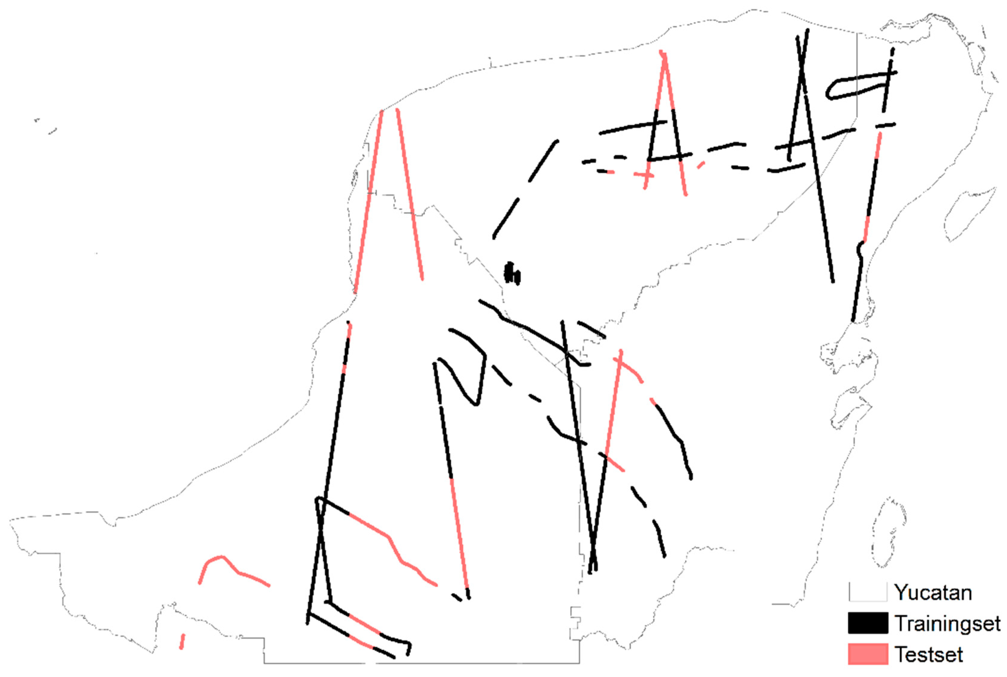
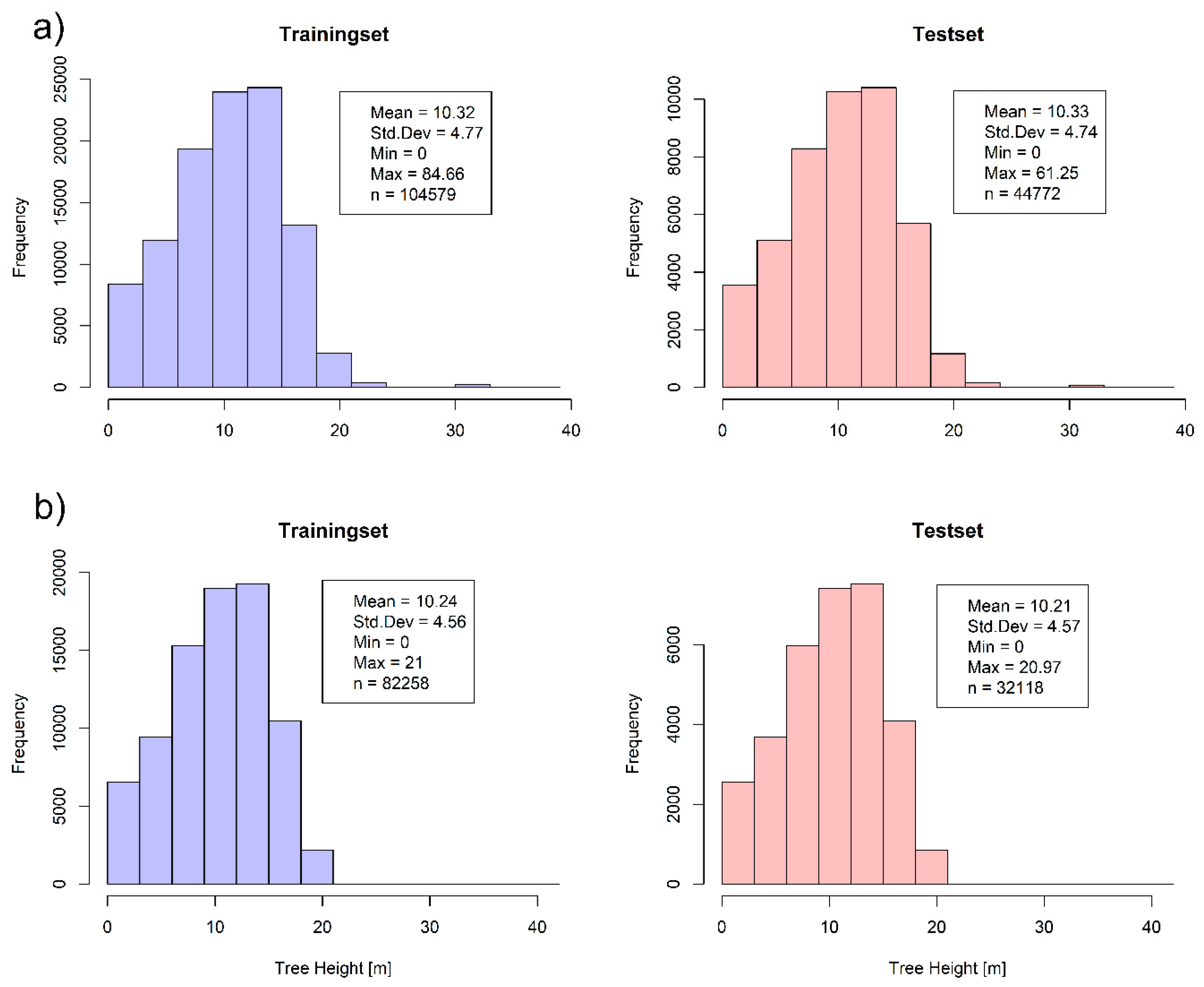
For model training and validation of SAR-based estimates, we applied two different splitting methods of the reference data (i.e., LiDAR-based vegetation height). For both approaches, 70% of the reference data were selected for model training (calibration) and the remaining 30% were used for testing (validation). In the first approach, we applied stratified random sampling, i.e., the data were split based on value intervals with ignoring spatial location of the samples. For this, intervals of 3 m were selected, i.e., 70/30 partition for each 3 m height class. We used intervals of 3 m as a trade-off between a sufficient number of samples for each height class and small enough bins to ensure the intra-class similarity. This splitting approach does not consider spatial autocorrelation between the training and test datasets, which generally results in overoptimistic model prediction statistics [58]. Therefore, in the second splitting approach, we divided the reference data based on their spatial location using k-means clustering of spatial coordinates (i.e., latitude and longitude) (Figure 3) using the R package “sperrorest” [58]. The first splitting approach will hereafter be called “stratified random sampling”, while the second splitting approach will be called “spatial sampling”. After data splitting using a “stratified random sampling” approach, the value distribution in training and test dataset is similar (Figure 4a). In “spatial sampling” after data splitting based on their geographical location, we fit the histograms of training and test data to each other, to ensure that value distribution in both datasets is similar, and the differences in the model’s predictive performance are from spatial autocorrelation and not from different value distributions. For this, the number of samples for specific 3 m height classes have been reduced until similar height distributions in the training and test datasets are reached (Figure 4b).
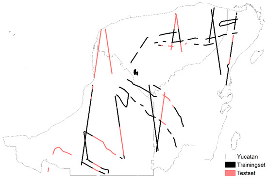
Figure 3.
Location of training and validation data using the “spatial sampling” approach of the LiDAR metric p100. Black stripes represent model training data; red stripes represent validation data.
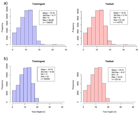
Figure 4.
Histograms of LiDAR-based vegetation height data used for training and test using (a) “stratified random sampling” (i.e., based on value intervals while ignoring spatial location) and (b) “spatial sampling” (i.e., based on spatial location).
2.4. Estimation of Vegetation Height from SAR Data
To estimate vegetation height using PALSAR-2 L-band backscatter, we applied different scenarios comprising two splitting approaches of reference data (i.e., “stratified random sampling” and “spatial sampling”) and two sets of input variables (i.e., ScanSAR and FBD mosaics). For all scenarios, the estimation of vegetation height was performed using a machine learning algorithm, namely Random Forests (RF) [59]. This machine learning algorithm generates an ensemble of regression trees with a random selection of predictors at each node as well as with a random subset of samples for each tree to prevent overfitting. To calculate a single estimate, the predictions of each regression tree are averaged [59]. We selected RF, since it is computationally efficient and has already been successfully applied to map vegetation structure metrics over large areas (e.g., AGB, vegetation height) with high retrieval accuracy (e.g., [37,60,61,62]). We generated RF models with 500 regression trees.
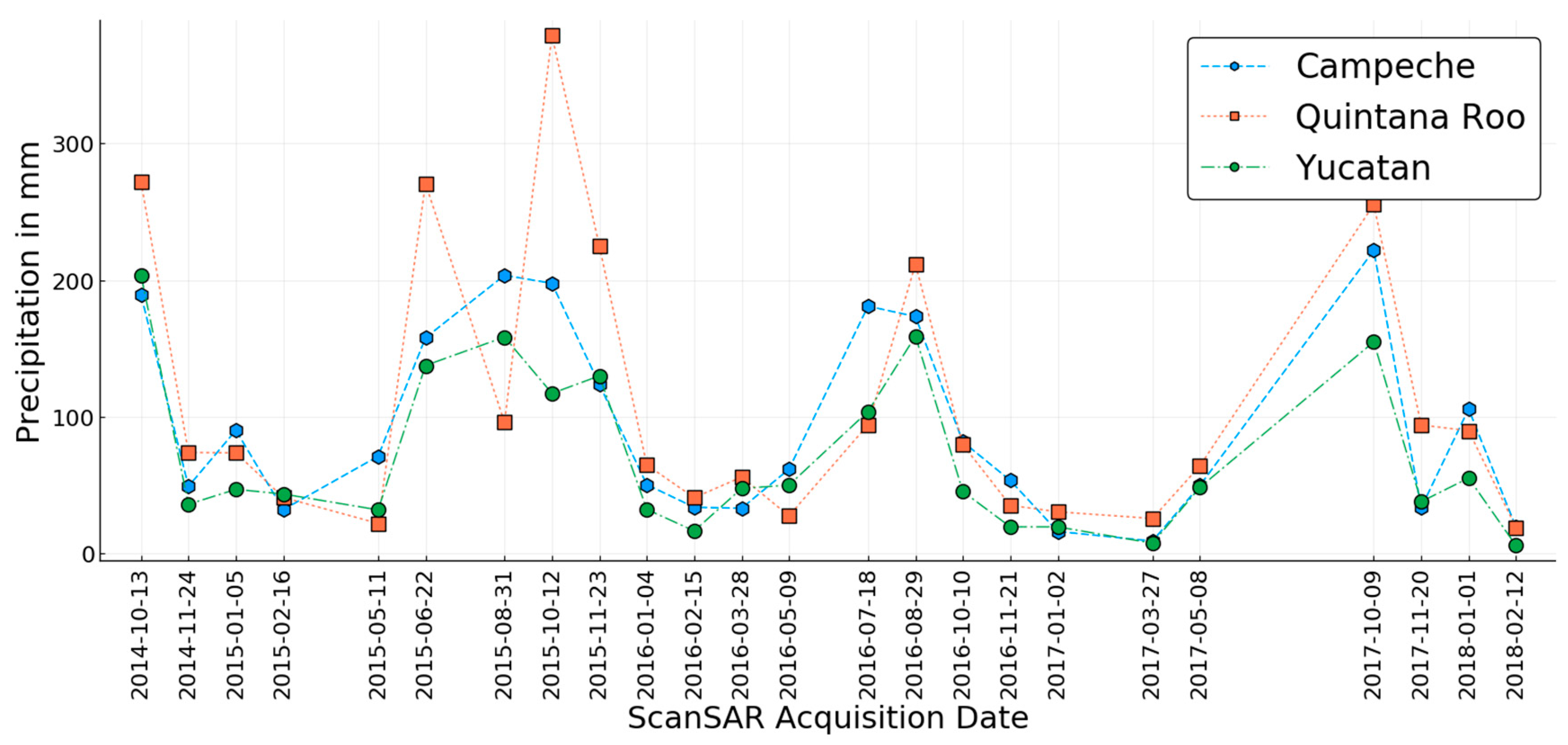
We furthermore investigated the impact of multi-temporal combination of ScanSAR data on the model’s predictive performance. Therefore, we modelled vegetation height using a different number of input layers. The acquisition date of a single ScanSAR mosaic can be found in Figure 5 (note: a single mosaic can be comprised of different ScanSAR products with slightly different acquisition dates (+/− one week from the reference date in Figure 5).We first estimated vegetation height with the first four ScanSAR scenes from2014–2015 (i.e., mosaics from 13 October 2014 to 16 February 2015 (Figure 5)) and added four further scenes at each step, i.e., we estimated vegetation height using 4, 8, 12, 16, 20 and 24 ScanSAR mosaics. The reference data were split using “stratified random sampling” and “spatial sampling” with 100 repetitions, i.e., the training and testing data were selected 100 times using both approaches to get reliable goodness-of-fit statistics (i.e., R2 and RMSE). Additionally, we performed the same steps for speckle unfiltered ScanSAR data to show the effect of speckle filtering.
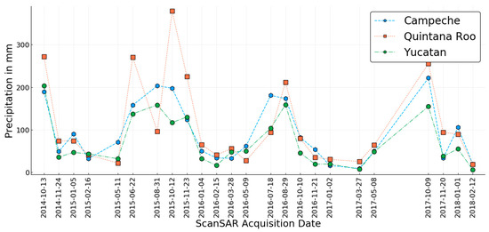
Figure 5.
Acquisition dates of the ScanSAR mosaics with corresponding monthly precipitation for the three federal states from [46].
Finally, we examined the impact of the number of training samples on the model prediction performance. Therefore, from the training set, 1%, 5%, and every decile (i.e., 10%, 20% ... 90%) of the data were sampled randomly 100 times and model performance statistics (i.e., R2 and RMSE) for each scenario were analysed. The validation dataset from “stratified random sampling” and “spatial sampling” (e.g., red stripes in Figure 3) remained unchanged.
3. Results
3.1. Estimation of Vegetation Height from SAR Data
We first sought to determine the merit of multi-temporal ScanSAR mosaics compared to the annual global FBD mosaics to map vegetation height. To examine this, we modelled vegetation height using ScanSAR and FBD mosaics separately. As described above, we applied two validation approaches, i.e., “stratified random sampling” and “spatial sampling” of reference data.
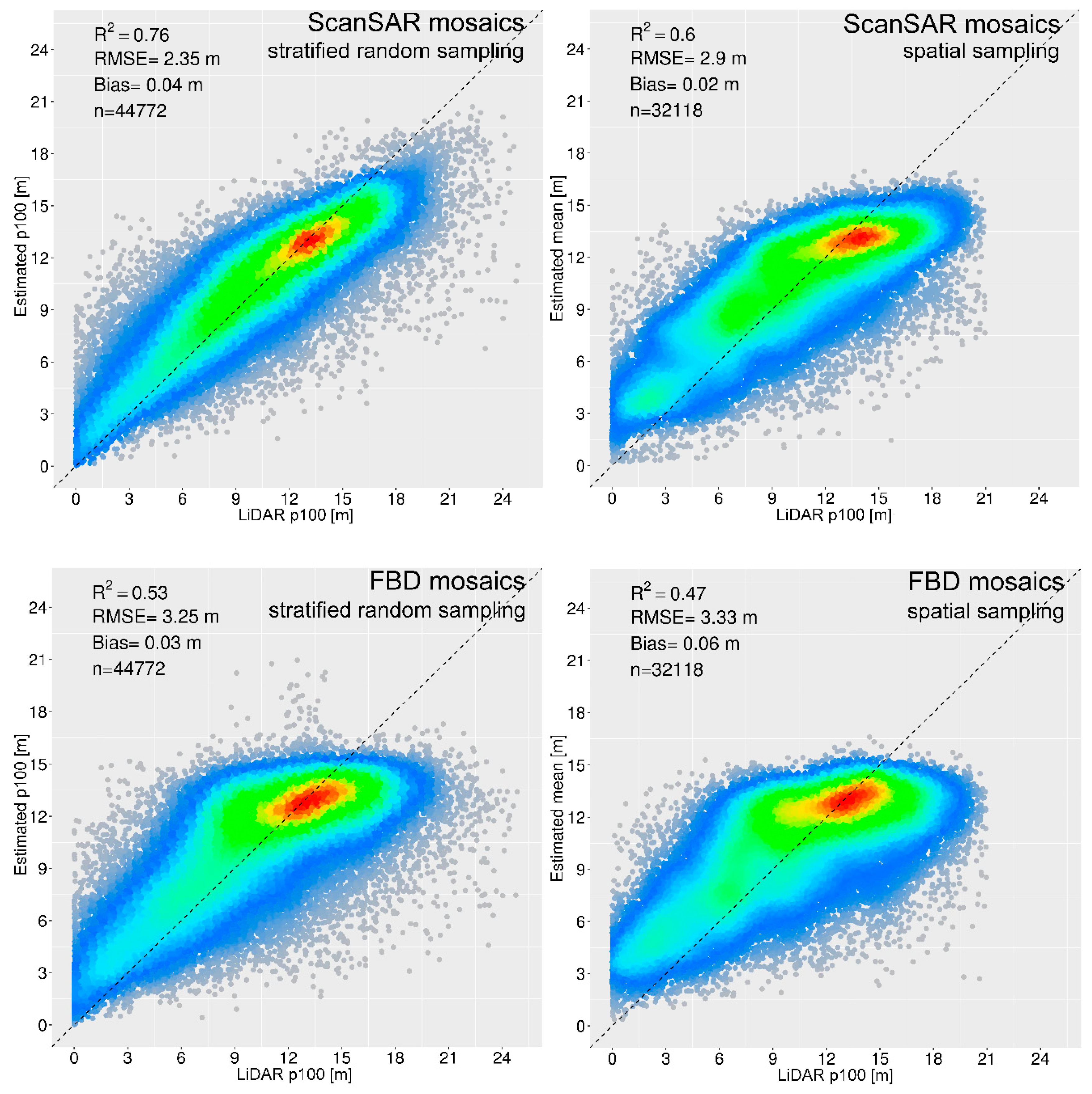
The results based on the “stratified random sampling” approach provide higher goodness-of-fit statistics (R2 and RMSE) compared to the “spatial sampling” approach for different sets of input variables (i.e., ScanSAR and FBD mosaics) (Figure 6). This is caused by the spatial autocorrelation of reference data, which is ignored in the “stratified random sampling” approach. In contrast, the “spatial sampling” validation considers this effect, providing a more realistic estimation of the model’s predictive performance [58], and might contribute to building a more robust predictive model. Furthermore, in the “spatial sampling” validation, the effect of over- and underestimations at low and high ranges, respectively, is more apparent compared to “stratified random sampling”. The effect of over- and underestimations at both ends have been reported in many studies that have applied an ensemble of regression trees (e.g., Random Forests) [39,63,64].
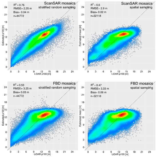
Figure 6.
ScanSAR (above) and FBD (bottom)-based vegetation height estimates plotted against LiDAR p100 metric. The training and test data were split using “stratified random sampling” (left) and “spatial sampling” (right). ScanSAR mosaics (24 scenes) show higher retrieval accuracy compared to FBD mosaics (3 scenes) due to a larger number of SAR images. The “stratified random sampling” approach shows higher goodness-of-fit statistics compared to the “spatial sampling” approach due to spatial autocorrelation between training and test data.
Moreover, the FBD-based vegetation height estimates are more biased at low and high ranges compared to the results based on ScanSAR mosaics for both validation scenarios (Figure 6). In other words, FBD-based vegetation height estimates tend to average height values of the training data. In the difference map between the two products (Figure 7), the FBD height possesses greater values in the areas with small vegetation (e.g., the northern part of the peninsula) compared to the ScanSAR-based product (i.e., it shows a larger overestimation), while in the intact areas (e.g., the Calakmul Biosphere Reserve) the FBD height exhibits lower values than in the ScanSAR height (i.e., it shows a larger underestimation).
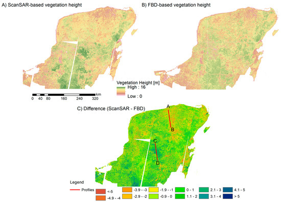
Figure 7.
Vegetation height estimates based on ScanSAR (A) and FBD (B) mosaics using the “spatial sampling” approach. The difference map (C) between the two products depicts disagreements in areas with low (northern part) and tall trees (central and southern parts). The height values over the two red transects (A-B profile and C-D profile) are shown in Figure 8. White gaps in the ScanSAR-based vegetation height map resulted from the gaps in the ScanSAR backscatter mosaics.
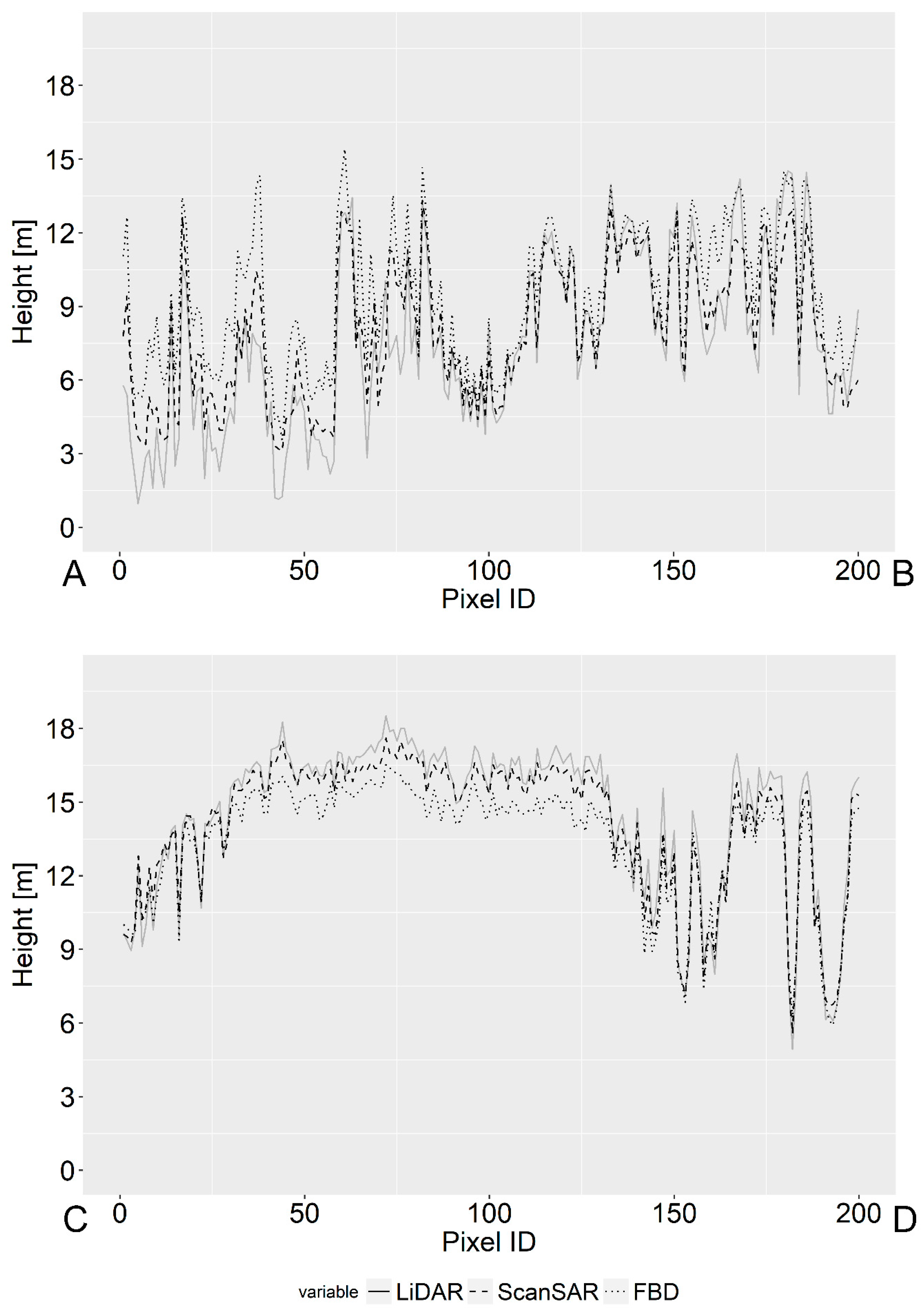
For areas with obvious disagreements between the two maps and where LiDAR data were available, transects of vegetation height (red stripes at the bottom of Figure 7) were generated (Figure 8). Compared to the LiDAR measurements, both SAR-based vegetation height maps show an overestimation of small vegetation and an underestimation of tall vegetation. The over- und underestimation at both ends (small and large trees) is partly caused by a tree-based regression (e.g., Random Forests and Cubist), where single predictions of each tree are averaged. Thus, height at low and high range tends to a mean value. Larger bias is observed for the FBD-based estimates (Figure 8). Accordingly, the increasing number of spatial predictors results in a reduction of the bias at both ends (i.e., the lowest and highest vegetation heights). Moreover, a lower deviation from LiDAR height for the A-B transect between pixel IDs 80–150 (Figure 8) can be observed. This is caused by the fact that this part of the LiDAR transect was used for model training, while other parts are independent (Figure 3 and Figure 8).
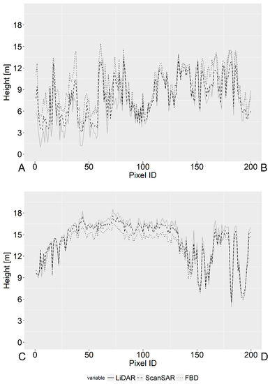
Figure 8.
Transects of the vegetation height of the three products over areas with small (upper profile) and tall trees (bottom profile). The upper image shows vegetation height for the transect A-B in the northern part of the peninsula (Figure 7), while the bottom image shows vegetation height for the transect C-D in the central part of the peninsula (Figure 7). The FBD-based map overestimated height in areas with small vegetation and underestimated in areas with tall vegetation more noticeably compared to the ScanSAR-based map. For visualisation reasons, every 5 pixels from north to south was averaged.
3.2. Impact of Number of L-Band Observations on Model’s Predictive Performance
Here, we analysed the influence of the number of spatial predictors on model prediction performance. For this analysis, we used ScanSAR mosaics only. As mentioned in Section 2.4, the reference data were divided into training and test data using “stratified random sampling” and “spatial sampling” with 100 repetitions. Furthermore, to show the effect of a speckle filter on the model’s predictive performance, unfiltered and multi-temporal speckle-filtered SAR data after [56] were used as predictive variables. The models based on “stratified random sampling” demonstrate a steady increase of R² and decrease of RMSE using both unfiltered and filtered SAR data (Figure 9 upper and bottom left). Moreover, the results based on the filtered SAR data possess much higher R² and lower RMSE compared to the results from unfiltered SAR data. The increase of R2 and decrease of RMSE from 4 to 8 scenes and further is much stronger in the models based on speckle-filtered SAR data. This is most likely caused by the fact that the applied filter uses a 7 × 7 moving window and thus strengthens the spatial autocorrelation between training and test data.
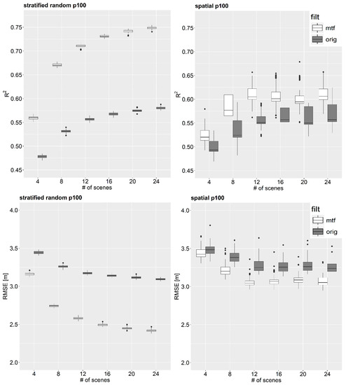
Figure 9.
Impact of number of scenes on model prediction performance using “stratified random sampling” (left) and “spatial sampling” (right) for multi-temporal Quegan speckle-filtered data (“mtf”, white boxplots) and unfiltered ScanSAR data (“orig”, dark-grey boxplot).
Another observation is that the variance of the model statistics based on “stratified random sampling” is much lower compared to the model statistics based on “spatial sampling”. Considering the models based on “spatial sampling”, those based on filtered data possess higher R2 and lower RMSE compared to those based on unfiltered SAR data (Figure 9 upper and bottom right). However, the differences in the statistics are not as high as in the “stratified random sampling” models. This confirms that the differences between the results based on filtered and unfiltered SAR data using “stratified random sampling” are caused by the spatial autocorrelation of the reference data. Finally, it can be observed that for more than 12 scenes, further increment of acquisitions does not result in further improvement of R2 and RMSE.
3.3. Impact of Number of Samples on Model Prediction Performance
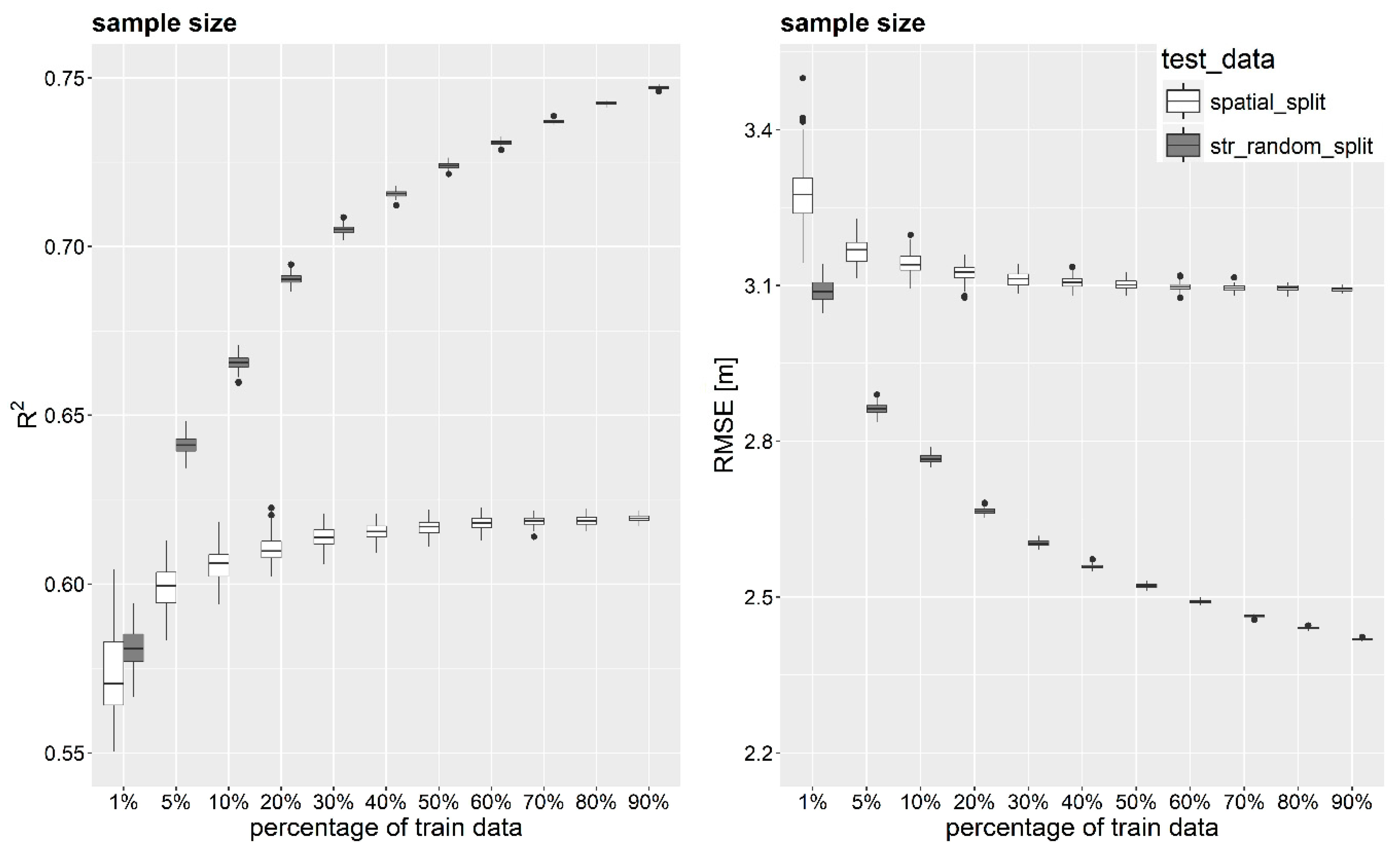
To test the impact of number of training samples on model’s predictive performance, the test data from both sampling strategies remained unchanged, while training set from both sampling strategies were sampled randomly 100 times with 1%, 5%, and every decile of the data. According to Figure 10 (dark-grey boxplots), for the “stratified random sampling” scenario, an increasing number of training data results in a steady improvement of the goodness-of-fit statistics (i.e., increase of R2 of about 27% and decrease of RMSE of about 22%). This is again caused by the spatial autocorrelation between training and test data, i.e., with an increasing number of training data, the probability to be adjoined with test data increases, resulting in continuous improvement of retrieval accuracies. However, if spatial autocorrelation is considered (i.e., the “spatial sampling” scenario), the model’s predictive performance saturates with an increasing number of training samples (Figure 10, white boxplots). With an increasing number of training data in the “spatial sampling” scenario, the model performance is enhanced up to a threshold of 20% of the training data, and very slightly afterwards. Additionally, the variance in the model statistics decreases with an increasing number of training samples. Based on the results, a threshold of around 20% of training data represents a plausible trade-off between model efficiency and data collection effort. 20% of training data corresponds here to 20,000 1-ha samples.
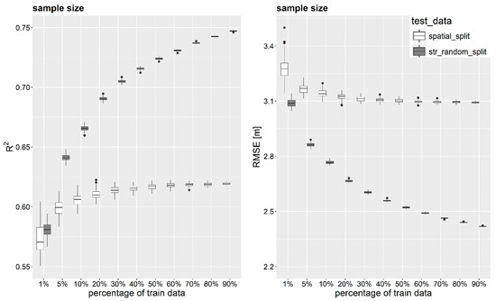
Figure 10.
Impact of sample quantity on model prediction performance using “stratified random sampling” (dark-grey boxplot) and “spatial sampling” (white boxplot). With an increasing number of training samples, the model performance increases continuously for “stratified random sampling” and saturates for “spatial sampling”. 1% of training data corresponds to 1000 1-ha samples.
4. Discussion and Summary
We examined the potential of multi-temporal L-band SAR backscatter to estimate vegetation height. Additionally, we investigated the impact of the number of spatial predictors and training samples on the model’s predictive performance given that the dataset is characterised by spatial autocorrelation.
This study has three main implications. First, we showed the value of multi-temporal L-band SAR backscatter for estimation of vegetation height. It is well known that, depending on forest structure, L-band SAR backscatter saturates in dense forests at biomass levels around 100 t/ha [65,66,67]. Our results indicate that including more L-band observations in a statistical model can partly help to reduce under- and overestimation at low and high ranges of a forest parameter, respectively (Figure 8). These results are in agreement with previous studies reporting that the usage of multi-temporal L- and C-band SAR data improves retrieval accuracies of growing stock volume and AGB [4,8,23,68,69]. We found, however, that after a specific number of observations, the model’s predictive performance is not further enhanced. In our case, using 12 dual-polarised L-band SAR observations, we estimated vegetation height with similar retrieval accuracies as using 24 dual-polarised L-band SAR observations (Figure 9). Obviously, 10–12 ScanSAR observations are sufficient to represent the multi-seasonal conditions of the forest vegetation over one year including dry and wet conditions at different phenological stages (i.e., leaf-off/leaf-on). According to our findings, the integration of 12 additional ScanSAR scenes does not lead to further prediction improvements. Hence, no relevant additional information can be gained from these images.
Second, spatial autocorrelation in the training and test dataset must be considered to provide a realistic predictive performance of the model. In the case where spatial autocorrelation in the reference data is ignored, estimation of the model’s performance is overoptimistic, caused by spatial autocorrelation between training and test data [58]. Moreover, ignoring spatial autocorrelation between training and test data can lead to incorrect conclusions, e.g., an increasing number of spatial predictors and/or training samples leads to steady improvements of the model’s predictive performance.
Third, an increasing number of training samples leads to improvements in the model’s predictive performance, but it saturates at a specific percentage of training samples. In contrast, Xu et al. [39] reported steady improvements of model performance with an increasing number of training samples in tropical forests. Garcia et al. [38] showed that retrieval accuracies were enhanced and saturated at a different percentage of training samples depending on forest structure (i.e., temperate broadleaf, mixed or coniferous forests). Nonetheless, neither study split the training and test data using geographical location of them, which might result in an overoptimistic model performance due to the likely spatial autocorrelation. In our study, using 20% of the training data was sufficient to get a similar level of accuracy as using 100% of the training data (Figure 6 and Figure 10). 20% of the training data represents 20,000 1-ha samples, though it is still a large number of training data. In any case, it is crucial that training samples represent the entire range of values (in our case vegetation height) from different forest types (i.e., deciduous and evergreen forests) of the study area.
As expected, speckle filtering of the SAR images resulted in a better retrieval accuracy. However, using a speckle filter based on a moving window approach strengthens the spatial autocorrelation in the reference data. Nowadays, with the increasing availability of SAR time series (e.g., Sentinel-1), novel approaches that rely on temporal patterns only can be applied to suppress speckle and preserve spatial details without spatial blurring [70]. Furthermore, since the difference in acquisition time between LiDAR and SAR data is between one to five years, significant changes (caused, e.g., by fire or deforestation) within the LiDAR transects might have occurred, which together with forest growth reduce model’s predictive performance [71].
As shown in several studies [38,39,63,71,72], retrieval accuracies of forest structure parameters can be improved by including additional information from optical remote sensing data, i.e., Landsat or Sentinel-2 surface reflectance, and digital surface model (e.g., SRTM DEM). Nevertheless, in this study, we analysed the performance of multi-temporal L-band backscatter data only for the estimation of vegetation height. Since vegetation height correlates with other forest parameters (e.g., AGB, tree canopy cover) [40,41,42], we can assume that similar results can be achieved for the estimation of AGB and tree canopy cover using multi-temporal dual-polarised L-band SAR backscatter.
5. Conclusions
ALOS-2 PALSAR-2 ScanSAR data provide time series of dual-polarised L-band observations (~10 observations per year) over wider areas (i.e., 350 km) at medium spatial resolution (i.e., 50 m), which is crucial for land monitoring at national or continental scales. In this study, we investigated the potential of this dataset to map vegetation height over tropical deciduous and evergreen forests of the Yucatan peninsula, Mexico. For this, we used airborne LiDAR-based vegetation height for the training of L-band backscatter using the Random Forests algorithm. Specifically, we examined the value of multi-temporal L-band data for the estimation of vegetation height taking the spatial autocorrelation between training and test data into account. Our results indicate that ignoring spatial autocorrelation between training and test data lead to an overoptimistic model’s predictive performance. Accordingly, a spatial splitting of the reference data into training and test data should be preferred to provide realistic retrieval accuracies. Moreover, based on this analysis, we determined an optimal number of L-band observations and training samples as a trade-off between retrieval accuracies and data collection effort.
Open data policies such as those of the ESA and NASA stimulate development of novel approaches based on these data (e.g., Landsat, Sentinels). Bearing in mind new L-band missions in near future (ALOS-4, NISAR, SAOCOM, Tandem-L) that will provide time series of L-band observations, open L-band PALSAR-2 ScanSAR data for the scientific community would foster further development of innovative algorithms for forest monitoring including mapping of forest structure parameters and detection of deforestation and forest degradation over large areas to support international climate initiatives (e.g., UN Reducing Emissions from Deforestation and Forest Degradation+ programme).
Author Contributions
M.U. and C.T. conceived and designed the experiments; M.U. performed the experiments; M.U. and F.C. analysed the data; M.U. wrote the paper; all co-authors assisted the lead author in writing and revising the manuscript. All authors read and approved the final manuscript.
Funding
M.U. was funded by the International Max Planck Research School for Global Biogeochemical Cycles. This work was partly funded by the German Aerospace Center (DLR) in the Sentinel4REDD project (FKZ: 50EE1540).
Acknowledgments
M.U. conducted this work under the International Max Planck Research School for Global Biogeochemical Cycles and acknowledges its funding and support. This work has been undertaken within the framework of the JAXA Kyoto & Carbon Initiative. ALOS PALSAR mosaic data were available from ©JAXA PALSAR MOSAIC 2014. The authors would like to thank JAXA for providing ALOS-2 PALSAR-2 ScanSAR data and NASA for providing airborne LiDAR data.
Conflicts of Interest
The authors declare no conflict of interest. The funders had no role in the design of the study; in the collection, analyses, or interpretation of data; in the writing of the manuscript, and in the decision to publish the results.
References
- Lefsky, M.A.; Cohen, W.B.; Harding, D.J.; Parker, G.G.; Acker, S.A.; Gower, S.T. Lidar remote sensing of above-ground biomass in three biomes. Glob. Ecol. Biogeogr. 2002, 11, 393–399. [Google Scholar] [CrossRef]
- Clark, M.L.; Clark, D.B.; Roberts, D.A. Small-footprint LiDAR estimation of sub-canopy elevation and tree height in a tropical rain forest landscape. Remote Sens. Environ. 2004, 91, 68–89. [Google Scholar] [CrossRef]
- Asner, G.P.; Hughes, R.F.; Vitousek, P.M.; Knapp, D.E.; Kennedy-Bowdoin, T.; Boardman, J.; Martin, R.E.; Eastwood, M.; Green, R.O. Invasive plants transform the three-dimensional structure of rain forests. Proc. Natl. Acad. Sci. USA 2008, 105, 4519–4523. [Google Scholar] [CrossRef] [PubMed]
- Cartus, O.; Santoro, M.; Kellndorfer, J. Mapping forest aboveground biomass in the Northeastern United States with ALOS PALSAR dual-polarization L-band. Remote Sens. Environ. 2012, 124, 466–478. [Google Scholar] [CrossRef]
- Lucas, R.; Armston, J.; Fairfax, R.; Fensham, R.; Accad, A.; Carreiras, J.; Kelley, J.; Bunting, P.; Clewley, D.; Bray, S. An evaluation of the ALOS PALSAR L-band backscatter—Above ground biomass relationship Queensland, Australia: Impacts of surface moisture condition and vegetation structure. IEEE J. Sel. Top. Appl. Earth Obs. Remote Sens. 2010, 3, 576–593. [Google Scholar] [CrossRef]
- Mitchard, E.T.A.; Saatchi, S.S.; Lewis, S.L.; Feldpausch, T.R.; Woodhouse, I.H.; Sonké, B.; Rowland, C.; Meir, P. Measuring biomass changes due to woody encroachment and deforestation/degradation in a forest–savanna boundary region of central Africa using multi-temporal L-band RADAR backscatter. Remote Sens. Environ. 2011, 115, 2861–2873. [Google Scholar] [CrossRef]
- Saatchi, S.; Marlier, M.; Chazdon, R.L.; Clark, D.B.; Russell, A.E. Impact of spatial variability of tropical forest structure on RADAR estimation of aboveground biomass. Remote Sens. Environ. 2011, 115, 2836–2849. [Google Scholar] [CrossRef]
- Santoro, M.; Beer, C.; Cartus, O.; Schmullius, C.; Shvidenko, A.; McCallum, I.; Wegmüller, U.; Wiesmann, A. Retrieval of growing stock volume in boreal forest using hyper-temporal series of Envisat ASAR ScanSAR backscatter measurements. Remote Sens. Environ. 2011, 115, 490–507. [Google Scholar] [CrossRef]
- Santos, J.R.; Freitas, C.C.; Araujo, L.S.; Dutra, L.V.; Mura, J.C.; Gama, F.F.; Soler, L.S.; Sant’Anna, S.J.S. Airborne P-band sar applied to the aboveground biomass studies in the Brazilian tropical rainforest. Remote Sens. Environ. 2003, 87, 482–493. [Google Scholar] [CrossRef]
- Tanase, M.A.; Panciera, R.; Lowell, K.; Tian, S.; Hacker, J.M.; Walker, J.P. Airborne multi-temporal L-band polarimetric SAR data for biomass estimation in semi-arid forests. Remote Sens. Environ. 2014, 145, 93–104. [Google Scholar] [CrossRef]
- Berninger, A.; Lohberger, S.; Stängel, M.; Siegert, F. SAR-based estimation of above-ground biomass and its changes in tropical forests of kalimantan using L- and C-band. Remote Sens. 2018, 10, 831. [Google Scholar] [CrossRef]
- Raney, R.K. RADAR fundamentals: Technical perspective. In Principles & Applications of Imaging RADAR. Manual of Remote Sensing; Henderson, F.M., Lewis, A.J., Eds.; John Wiley: New York, NY, USA, 1996; pp. 9–130. [Google Scholar]
- Le Toan, T.; Beaudoin, A.; Riom, J.; Guyon, D. Relating forest biomass to SAR data. IEEE Trans. Geosci. Remote Sens. 1992, 30, 403–411. [Google Scholar] [CrossRef]
- Lucas, R.M.; Moghaddam, M.; Cronin, N. Microwave scattering from mixed-species forests, Queensland, Australia. IEEE Trans. Geosci. Remote Sens. 2004, 42, 2142–2159. [Google Scholar] [CrossRef]
- Lee, J.-S.; Pottier, E. Polarimetric RADAR Imaging: From Basics to Applications; CRC Press: Boca Raton, FL, USA, 2009. [Google Scholar]
- Rauste, Y.; Hame, T.; Pulliainen, J.; Heiska, K.; Hallikainen, M. RADAR-based forest biomass estimation. Int. J. Remote Sens. 1994, 15, 2797–2808. [Google Scholar] [CrossRef]
- Watanabe, M.; Shimada, M.; Rosenqvist, A.; Tadono, T.; Matsuoka, M.; Shakil Ahmad, R.; Ohta, K.; Furuta, R.; Nakamura, K.; Moriyama, T. Forest structure dependency of the relation between L-band σ0 and biophysical parameters. IEEE Trans. Geosci. Remote Sens. 2006, 44, 3154–3165. [Google Scholar] [CrossRef]
- Askne, J.I.H.; Fransson, J.E.S.; Santoro, M.; Soja, M.J.; Ulander, L.M.H. Model-based biomass estimation of a hemi-boreal forest from multitemporal TanDEM-X acquisitions. Remote Sens. 2013, 5, 5574–5597. [Google Scholar] [CrossRef]
- Solberg, S.; Astrup, R.; Breidenbach, J.; Nilsen, B.; Weydahl, D. Monitoring spruce volume and biomass with InSAR data from TanDEM-X. Remote Sens. Environ. 2013, 139, 60–67. [Google Scholar] [CrossRef]
- Hajnsek, I.; Kugler, F.; Lee, S.-K.; Papathanassiou, K.P. Tropical-forest-parameter estimation by means of Pol-InSAR: The indrex-II campaign. IEEE Trans. Geosci. Remote Sens. 2009, 47, 481–493. [Google Scholar] [CrossRef]
- Papathanassiou, K.P.; Cloude, S.R. Single-baseline polarimetric SAR interferometry. IEEE Trans. Geosci. Remote Sens. 2001, 39, 2352–2363. [Google Scholar] [CrossRef]
- Dinh Ho Tong, M.; Thuy Le, T.; Rocca, F.; Tebaldini, S.; d’Alessandro, M.M.; Villard, L. Relating P-band synthetic aperture RADAR tomography to tropical forest biomass. IEEE Trans. Geosci. Remote Sens. 2014, 52, 967–979. [Google Scholar] [CrossRef]
- Antropov, O.; Rauste, Y.; Häme, T.; Praks, J. Polarimetric ALOS PALSAR time series in mapping biomass of boreal forests. Remote Sens. 2017, 9, 999. [Google Scholar] [CrossRef]
- Solberg, S.; Hansen, E.H.; Gobakken, T.; Næssset, E.; Zahabu, E. Biomass and InSAR height relationship in a dense tropical forest. Remote Sens. Environ. 2017, 192, 166–175. [Google Scholar] [CrossRef]
- Schlund, M.; von Poncet, F.; Kuntz, S.; Boehm, H.-D.V.; Hoekman, D.H.; Schmullius, C. TanDEM-X elevation model data for canopy height and aboveground biomass retrieval in a tropical peat swamp forest. Int. J. Remote Sens. 2016, 37, 5021–5044. [Google Scholar] [CrossRef]
- Santoro, M.; Cartus, O. Research pathways of forest above-ground biomass estimation based on SAR backscatter and interferometric SAR observations. Remote Sens. 2018, 10, 608. [Google Scholar] [CrossRef]
- Bucini, G.; Hanan, N.P.; Boone, R.B.; Smit, I.P.J.; Saatchi, S.S.; Lefsky, M.A.; Asner, G.P. Woody fractional cover in Kruger National Park, South Africa. In Ecosystem Function in Savannas; CRC Press: Boca Raton, FL, USA, 2010; pp. 219–237. [Google Scholar]
- Li, S.; Potter, C.; Hiatt, C.; Shupe, J. Fusion of hyperspectral and L-band SAR data to estimate fractional vegetation cover in a coastal california scrub community. J. Geophys. Remote Sens. 2012, 1, 1000104. [Google Scholar]
- Musick, H.B.; Schaber, G.S.; Breed, C.S. AIRSAR studies of woody shrub density in semiarid rangeland: Jornada Del Muerto, New Mexico. Remote Sens. Environ. 1998, 66, 29–40. [Google Scholar] [CrossRef]
- Urbazaev, M.; Thiel, C.; Mathieu, R.; Naidoo, L.; Levick, S.R.; Smit, I.P.J.; Asner, G.P.; Schmullius, C. Assessment of the mapping of fractional woody cover in Southern African savannas using multi-temporal and polarimetric ALOS PALSAR L-band images. Remote Sens. Environ. 2015, 166, 138–153. [Google Scholar] [CrossRef]
- Naidoo, L.; Mathieu, R.; Main, R.; Wessels, K.; Asner, G.P. L-band synthetic aperture RADAR imagery performs better than optical datasets at retrieving woody fractional cover in deciduous, dry savannahs. Int. J. Appl. Earth Obs. Geoinf. 2016, 52, 54–64. [Google Scholar] [CrossRef]
- Dong, J.; Xiao, X.; Sheldon, S.; Biradar, C.; Zhang, G.; Dinh Duong, N.; Hazarika, M.; Wikantika, K.; Takeuhci, W.; Moore, B., III. A 50-m forest cover map in Southeast Asia from ALOS/PalSAR and its application on forest fragmentation assessment. PLoS ONE 2014, 9, e85801. [Google Scholar] [CrossRef] [PubMed]
- Shimada, M.; Itoh, T.; Motooka, T.; Watanabe, M.; Shiraishi, T.; Thapa, R.; Lucas, R. New global forest/non-forest maps from ALOS PALSAR data (2007–2010). Remote Sens. Environ. 2014, 155, 13–31. [Google Scholar] [CrossRef]
- Thiel, C.J.; Thiel, C.; Schmullius, C.C. Operational large-area forest monitoring in Siberia using ALOS PALSAR summer intensities and winter coherence. IEEE Trans. Geosci. Remote Sens. 2009, 47, 3993–4000. [Google Scholar] [CrossRef]
- Thiel, C.; Drezet, P.; Weise, C.; Quegan, S.; Schmullius, C. RADAR remote sensing for the delineation of forest cover maps and the detection of deforestation. Forestry 2006, 79, 589–597. [Google Scholar] [CrossRef]
- Suzuki, R.; Kim, Y.; Ishii, R. Sensitivity of the backscatter intensity of ALOS/PalSAR to the above-ground biomass and other biophysical parameters of boreal forest in Alaska. Polar Sci. 2013, 7, 100–112. [Google Scholar] [CrossRef]
- Cartus, O.; Kellndorfer, J.; Rombach, M.; Walker, W. Mapping canopy height and growing stock volume using airborne LiDAR, ALOS PALSAR and landsat ETM+. Remote Sens. 2012, 4, 3320–3345. [Google Scholar] [CrossRef]
- García, M.; Saatchi, S.; Ustin, S.; Balzter, H. Modelling forest canopy height by integrating airborne LiDAR samples with satellite RADAR and multispectral imagery. Int. J. Appl. Earth Obs. Geoinf. 2018, 66, 159–173. [Google Scholar] [CrossRef]
- Xu, L.; Saatchi, S.S.; Yang, Y.; Yu, Y.; White, L. Performance of non-parametric algorithms for spatial mapping of tropical forest structure. Carbon Balance Manag. 2016, 11, 18. [Google Scholar] [CrossRef] [PubMed]
- Chave, J.; Andalo, C.; Brown, S.; Cairns, M.A.; Chambers, J.Q.; Eamus, D.; Folster, H.; Fromard, F.; Higuchi, N.; Kira, T.; et al. Tree allometry and improved estimation of carbon stocks and balance in tropical forests. Oecologia 2005, 145, 87–99. [Google Scholar] [CrossRef] [PubMed]
- Colgan, M.S.; Asner, G.P.; Swemmer, T. Harvesting tree biomass at the stand level to assess the accuracy of field and airborne biomass estimation in savannas. Ecol. Appl. 2013, 23, 1170–1184. [Google Scholar] [CrossRef] [PubMed]
- Saatchi, S.S.; Harris, N.L.; Brown, S.; Lefsky, M.; Mitchard, E.T.; Salas, W.; Zutta, B.R.; Buermann, W.; Lewis, S.L.; Hagen, S.; et al. Benchmark map of forest carbon stocks in tropical regions across three continents. Proc. Natl. Acad. Sci. USA 2011, 108, 9899–9904. [Google Scholar] [CrossRef] [PubMed]
- INEGI. Conjunto Nacional de Uso del Suelo y Vegetación a Escala 1:250,000, Serie iv; INEGI: Aguascalientes, Mexico, 2010. [Google Scholar]
- CONAFOR. Inventario Nacional Forestal y de Suelos. Informe 2004–2009; CONAFOR: Zapopan, Mexico, 2012. [Google Scholar]
- CSI, C. Srtm 90m Digital Elevation Database v4.1. Available online: http://www.cgiar-csi.org/data/srtm-90m-digital-elevation-database-v4-1 (accessed on 2 September 2016).
- SMN. Resumenes Mensuales de Temperaturas y Lluvia. Available online: https://smn.cna.gob.mx/es/climatologia/temperaturas-y-lluvias/resumenes-mensuales-de-temperaturas-y-lluvias (accessed on 5 June 2018).
- Urquiza-Haas, T.; Dolman, P.M.; Peres, C.A. Regional scale variation in forest structure and biomass in the Yucatan Peninsula, Mexico: Effects of forest disturbance. For. Ecol. Manag. 2007, 247, 80–90. [Google Scholar] [CrossRef]
- Cook, B.; Corp, L.; Nelson, R.; Middleton, E.; Morton, D.; McCorkel, J.; Masek, J.; Ranson, K.; Ly, V.; Montesano, P. Nasa goddard’s LiDAR, hyperspectral and thermal (G-LIHT) airborne imager. Remote Sens. 2013, 5, 4045–4066. [Google Scholar] [CrossRef]
- Evans, J.; Hudak, A.; Faux, R.; Smith, A.M. Discrete return LiDAR in natural resources: Recommendations for project planning, data processing, and deliverables. Remote Sens. 2009, 1, 776–794. [Google Scholar] [CrossRef]
- Næsset, E. Predicting forest stand characteristics with airborne scanning laser using a practical two-stage procedure and field data. Remote Sens. Environ. 2002, 80, 88–99. [Google Scholar] [CrossRef]
- Goetz, S.; Steinberg, D.; Dubayah, R.; Blair, B. Laser remote sensing of canopy habitat heterogeneity as a predictor of bird species richness in an eastern temperate forest, USA. Remote Sens. Environ. 2007, 108, 254–263. [Google Scholar] [CrossRef]
- NASA. Nasa G-LIHT Data. Available online: https://glihtdata.gsfc.nasa.gov/ (accessed on 5 June 2018).
- Rosenqvist, A.; Shimada, M.; Suzuki, S.; Ohgushi, F.; Tadono, T.; Watanabe, M.; Tsuzuku, K.; Watanabe, T.; Kamijo, S.; Aoki, E. Operational performance of the ALOS global systematic acquisition strategy and observation plans for ALOS-2 PALSAR-2. Remote Sens. Environ. 2014, 155, 3–12. [Google Scholar] [CrossRef]
- JAXA. New Global 25m-Resolution PALSAR-2/PALSAR Mosaic and Global Forest/Non-Forest Map. Available online: http://www.eorc.jaxa.jp/ALOS/en/palsar_fnf/data/index.htm (accessed on 31 July 2016).
- Quegan, S.; Le Toan, T.; Yu, J.J.; Ribbes, F.; Floury, N. Multitemporal ERS SAR analysis applied to forest mapping. IEEE Trans. Geosci. Remote Sens. 2000, 38, 741–753. [Google Scholar] [CrossRef]
- Quegan, S.; Yu, J.J. Filtering of multichannel SAR images. IEEE Trans. Geosci. Remote Sens. 2001, 39, 2373–2379. [Google Scholar] [CrossRef]
- Mathieu, R.; Naidoo, L.; Cho, M.A.; Leblon, B.; Main, R.; Wessels, K.; Asner, G.P.; Buckley, J.; Van Aardt, J.; Erasmus, B.F.N.; et al. Toward structural assessment of semi-arid African savannahs and woodlands: The potential of multitemporal polarimetric RADARSAT-2 fine beam images. Remote Sens. Environ. 2013, 138, 215–231. [Google Scholar] [CrossRef]
- Brenning, A. Spatial Cross-Validation and Bootstrap for the Assessment of Prediction Rules in Remote Sensing: The R Package ‘Sperrorest’. In Proceedings of the 2012 IEEE International Geoscience and Remote Sensing Symposium (IGARSS), Munich, Germany, 23–27 July 2012; pp. 5372–5375. [Google Scholar]
- Breiman, L. Random forests. Mach. Learn. 2001, 45, 5–32. [Google Scholar] [CrossRef]
- Avitabile, V.; Baccini, A.; Friedl, M.A.; Schmullius, C. Capabilities and limitations of landsat and land cover data for aboveground woody biomass estimation of uganda. Remote Sens. Environ. 2012, 117, 366–380. [Google Scholar] [CrossRef]
- Baccini, A.; Laporte, N.; Goetz, S.J.; Sun, M.; Dong, H. A first map of tropical Africa’s above-ground biomass derived from satellite imagery. Environ. Res. Lett. 2008, 3, 045011. [Google Scholar] [CrossRef]
- Baccini, A.; Goetz, S.J.; Walker, W.S.; Laporte, N.T.; Sun, M.; Sulla-Menashe, D.; Hackler, J.; Beck, P.S.A.; Dubayah, R.; Friedl, M.A.; et al. Estimated carbon dioxide emissions from tropical deforestation improved by carbon-density maps. Nat. Clim. Chang. 2012, 2, 182–185. [Google Scholar] [CrossRef]
- Cartus, O.; Kellndorfer, J.; Walker, W.; Franco, C.; Bishop, J.; Santos, L.; Fuentes, J. A national, detailed map of forest aboveground carbon stocks in Mexico. Remote Sens. 2014, 6, 5559–5588. [Google Scholar] [CrossRef]
- Urbazaev, M.; Thiel, C.; Cremer, F.; Dubayah, R.; Migliavacca, M.; Reichstein, M.; Schmullius, C. Estimation of forest aboveground biomass and uncertainties by integration of field measurements, airborne LiDAR, and SAR and optical satellite data in Mexico. Carbon Balance Manag. 2018, 13, 5. [Google Scholar] [CrossRef] [PubMed]
- Mermoz, S.; Le Toan, T.; Villard, L.; Réjou-Méchain, M.; Seifert-Granzin, J. Biomass assessment in the cameroon savanna using ALOS PALSAR data. Remote Sens. Environ. 2014, 155, 109–119. [Google Scholar] [CrossRef]
- Mitchard, E.T.A.; Saatchi, S.S.; Gerard, F.F.; Lewis, S.L.; Meir, P. Measuring woody encroachment along a forest–savanna boundary in Central Africa. Earth Interact. 2009, 13, 1–29. [Google Scholar] [CrossRef]
- Yu, Y.; Saatchi, S. Sensitivity of L-band SAR backscatter to aboveground biomass of global forests. Remote Sens. 2016, 8, 522. [Google Scholar] [CrossRef]
- Santoro, M.; Eriksson, L.; Askne, J.; Schmullius, C. Assessment of stand-wise stem volume retrieval in boreal forest from JERS-1 L-band SAR backscatter. Int. J. Remote Sens. 2006, 27, 3425–3454. [Google Scholar] [CrossRef]
- Santoro, M.; Beaudoin, A.; Beer, C.; Cartus, O.; Fransson, J.E.S.; Hall, R.J.; Pathe, C.; Schmullius, C.; Schepaschenko, D.; Shvidenko, A.; et al. Forest growing stock volume of the northern hemisphere: Spatially explicit estimates for 2010 derived from Envisat ASAR. Remote Sens. Environ. 2015, 168, 316–334. [Google Scholar] [CrossRef]
- Cremer, F.; Urbazaev, M.; Berger, C.; Mahecha, M.D.; Schmullius, C.; Thiel, C. An image transform based on temporal decomposition. IEEE Geosci. Remote Sens. Lett. 2018, 15, 537–541. [Google Scholar] [CrossRef]
- Urbazaev, M.; Thiel, C.; Migliavacca, M.; Reichstein, M.; Rodriguez-Veiga, P.; Schmullius, C. Improved multi-sensor satellite-based aboveground biomass estimation by selecting temporally stable forest inventory plots using NDVI time series. Forests 2016, 7, 169. [Google Scholar] [CrossRef]
- Rodríguez-Veiga, P.; Saatchi, S.; Tansey, K.; Balzter, H. Magnitude, spatial distribution and uncertainty of forest biomass stocks in Mexico. Remote Sens. Environ. 2016, 183, 265–281. [Google Scholar] [CrossRef]
© 2018 by the authors. Licensee MDPI, Basel, Switzerland. This article is an open access article distributed under the terms and conditions of the Creative Commons Attribution (CC BY) license (http://creativecommons.org/licenses/by/4.0/).

