Fractal-Based Local Range Slope Estimation from Single SAR Image with Applications to SAR Despeckling and Topographic Mapping


Abstract

1. Introduction
2. Materials and Methods
2.1. Direct Model
2.1.1. Surface Model
- H: Hurst coefficient (0 < H < 1) related to the fractal dimension D = 3 − H;
- T: topothesy [m], i.e., the distance over which chords joining points on the surface have a surface-slope mean-square deviation equal to unity.
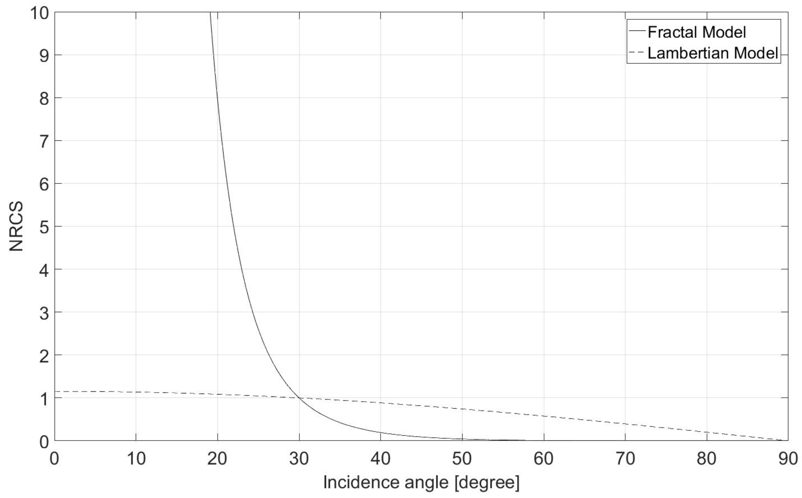
2.1.2. Scattering Model
2.1.3. Imaging Model
2.2. Model Inversion
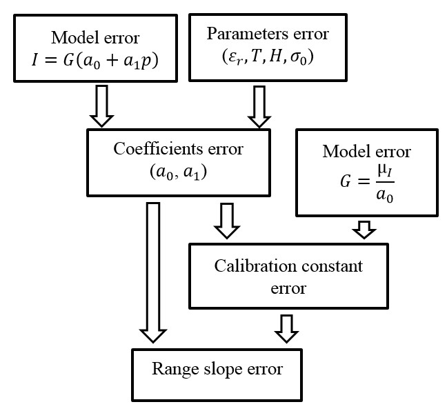
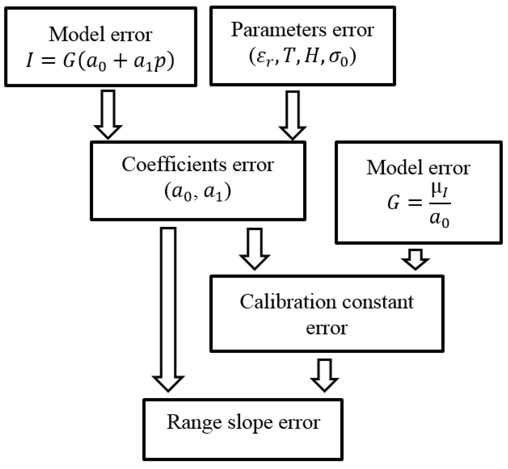
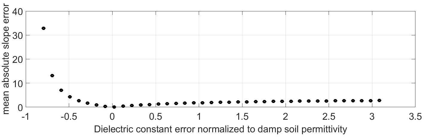
Error Source Evaluation
2.3. High-Level Products
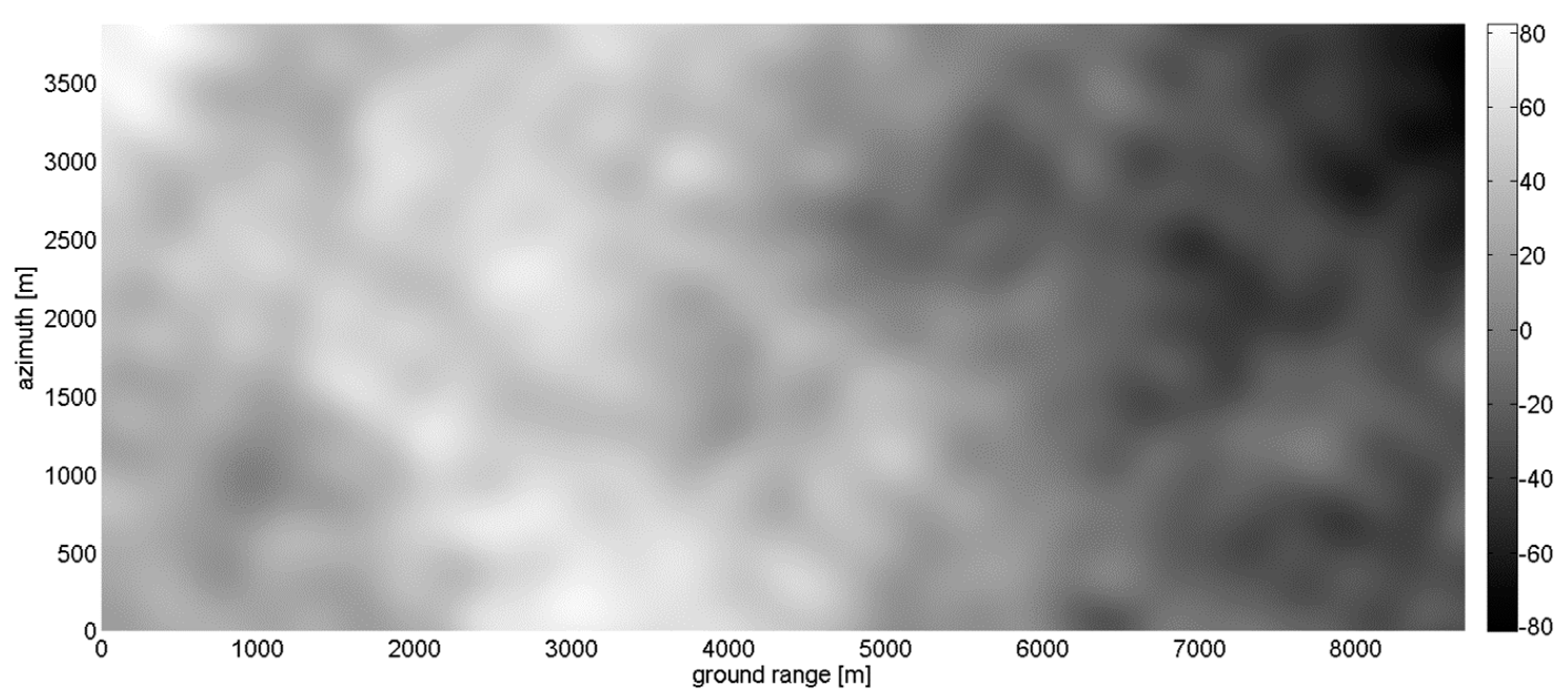
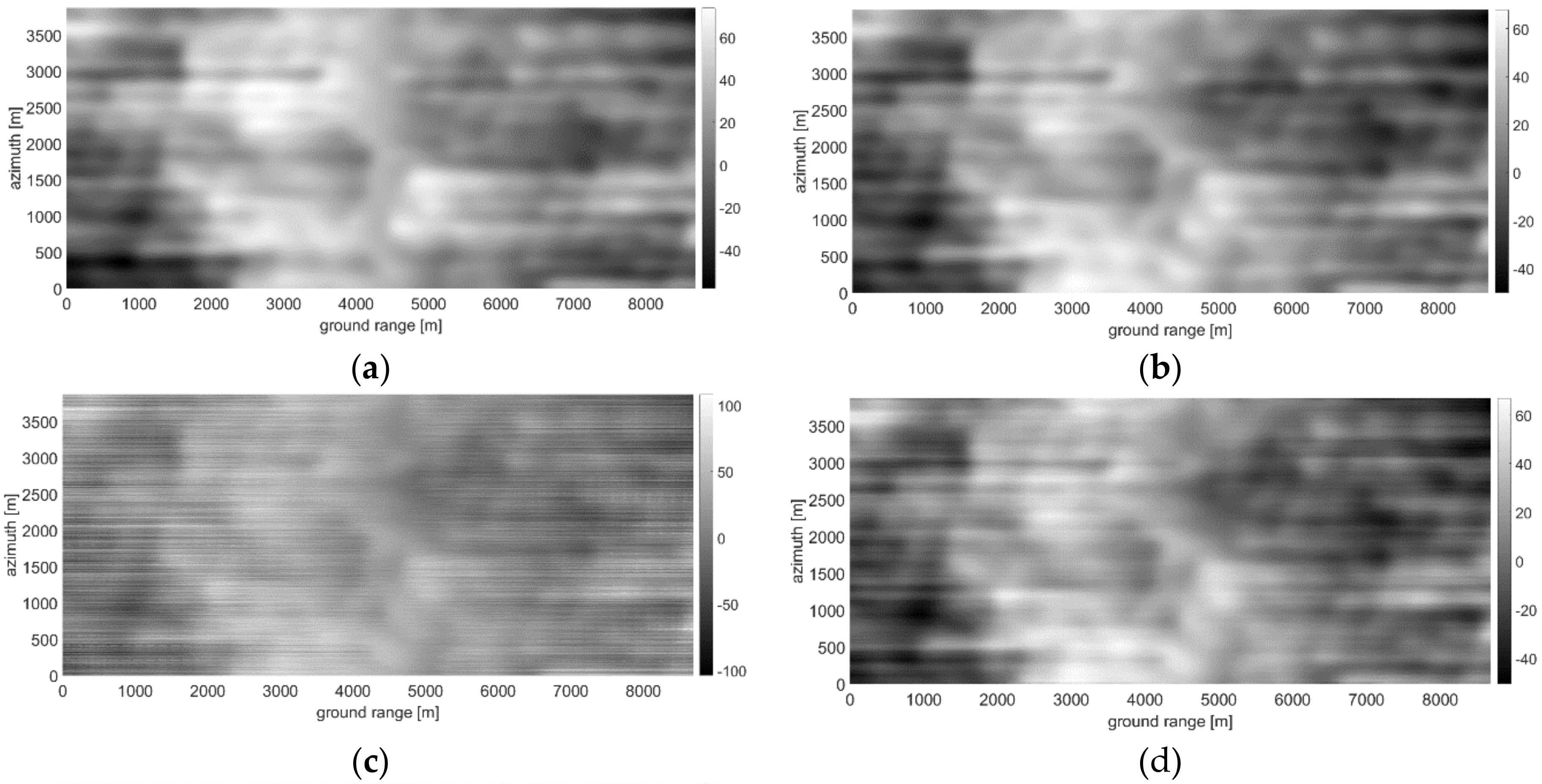
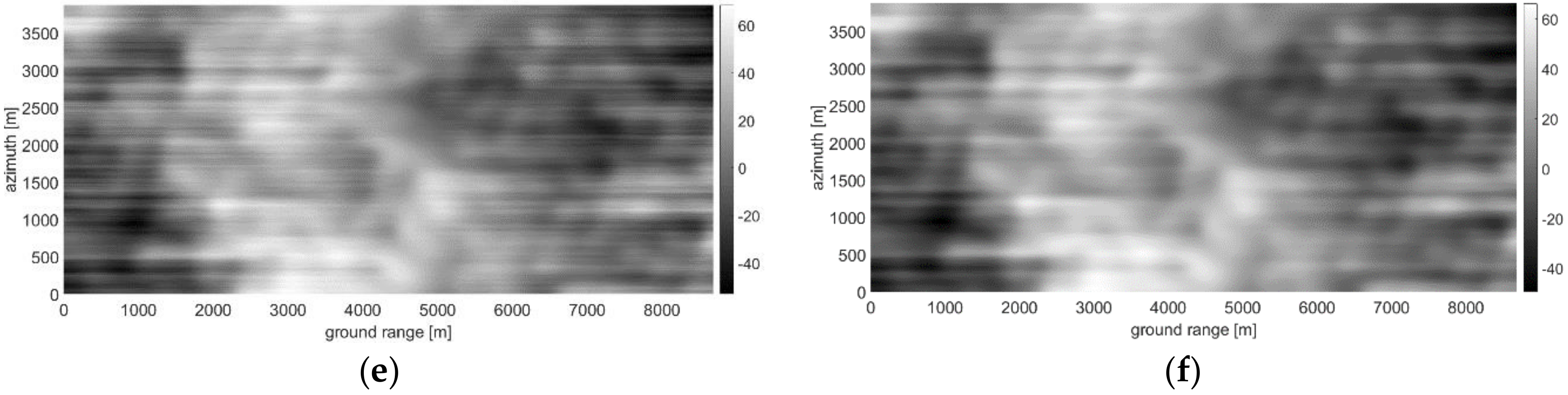
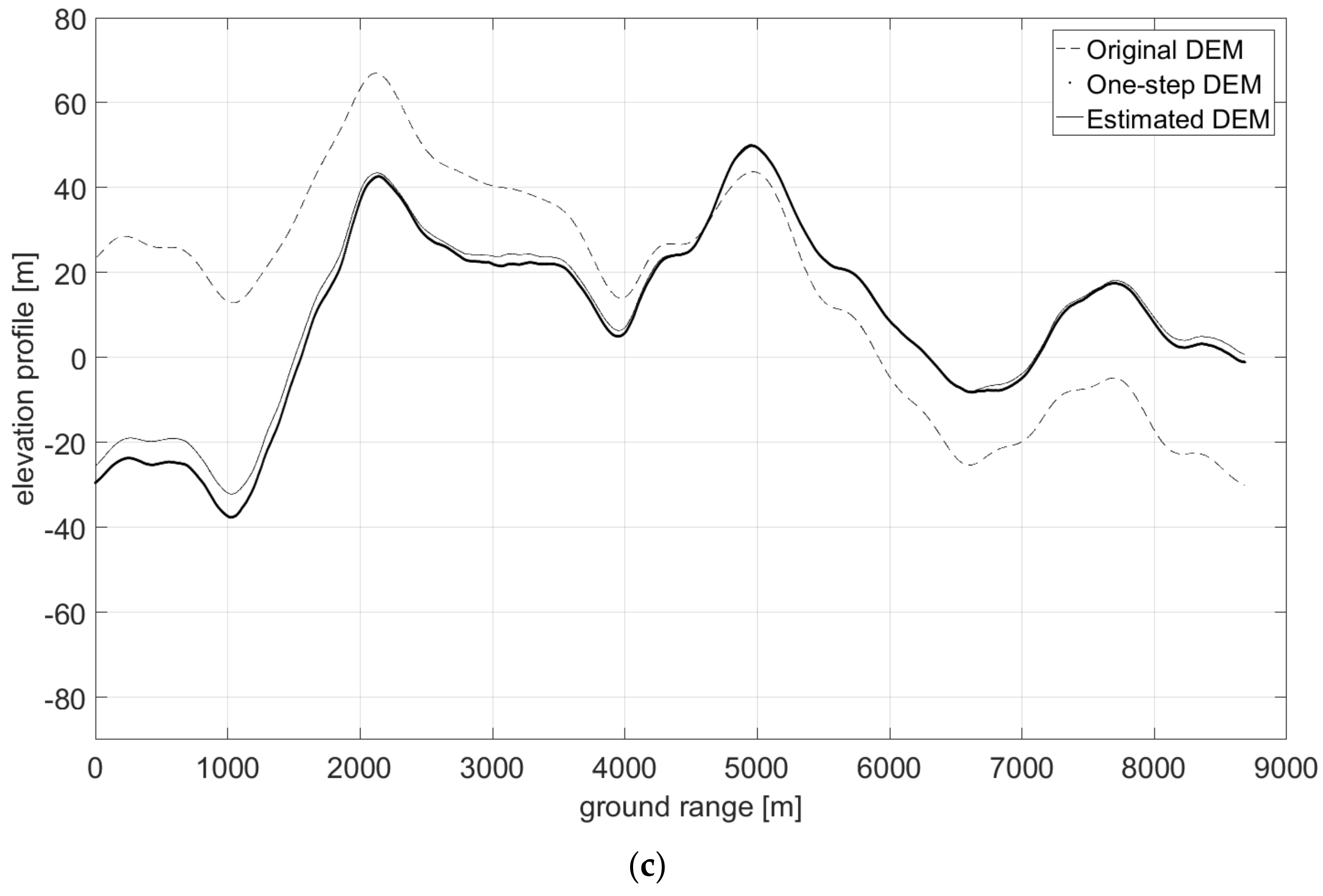
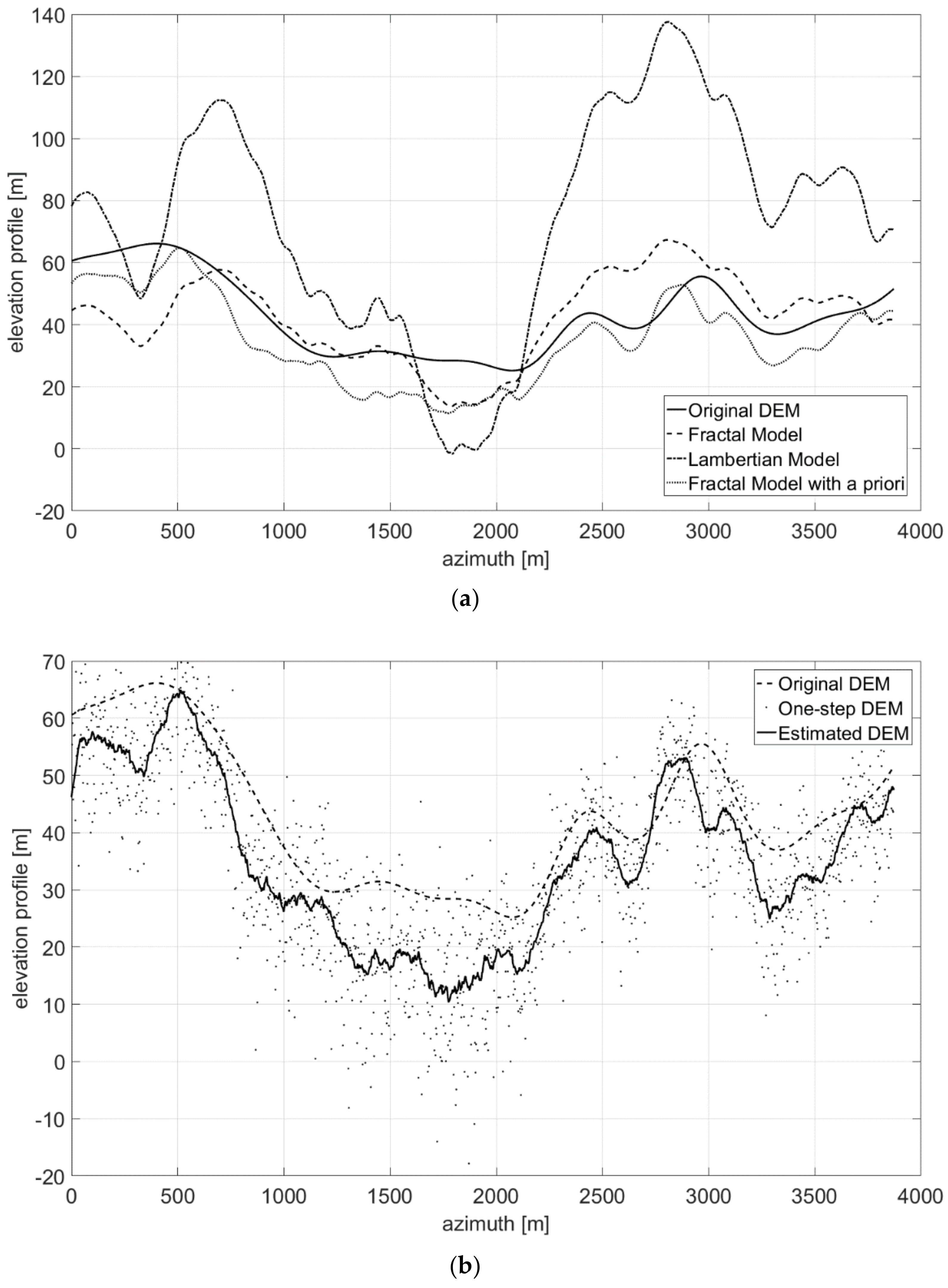
2.3.1. DEM Generation
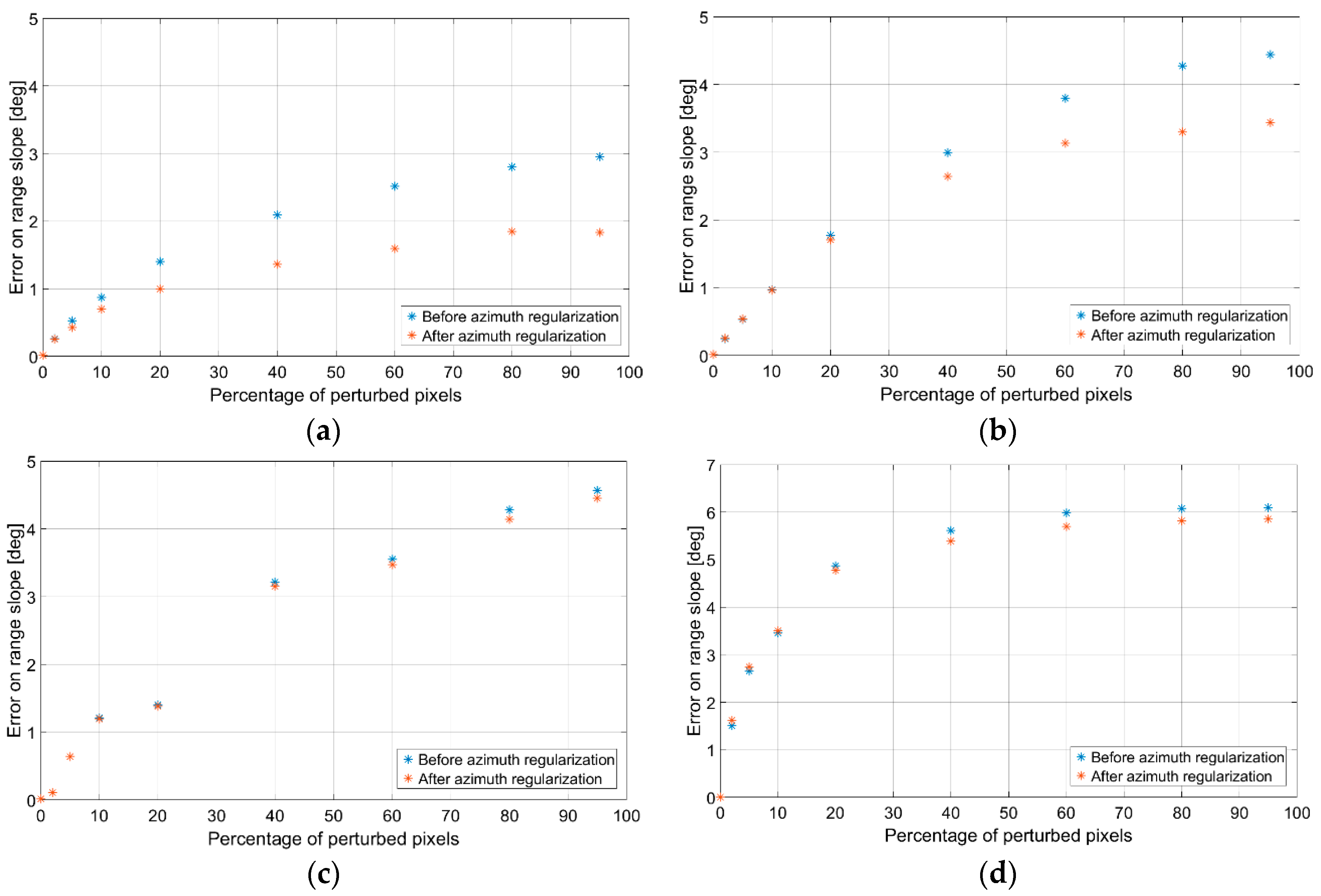
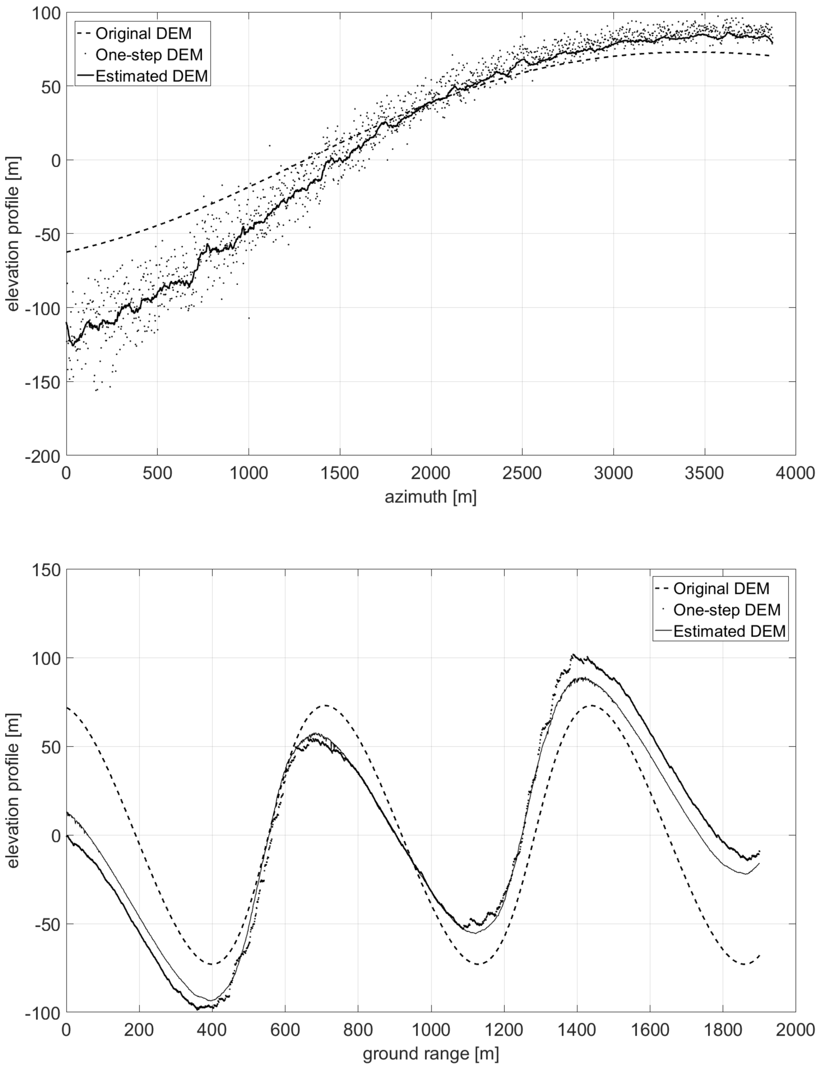
- First, neglecting the local azimuth slope q, it is possible to solve (11) for the unique unknown p, thus obtaining an initial estimate of the height map through slope integration in the range direction. Indeed, according to (11) image amplitude is linearly related to the range component of terrain slope, at least in a first-order approximation. Hence, individual SAR range lines can be independently integrated to generate elevation profiles.
- The raw guess of the DEM obtained in the first step does not account for azimuth slopes, so that the reconstructed DEM presents unnatural patterns along the range axis, due to independent range line integration. Therefore, the second step consists in a regularization procedure able to correct the integration errors, also taking into account the azimuth component of the slope q.
2.3.2. Scattering-Based Despeckling
3. Results and Discussion
3.1. Hypotheses Validation
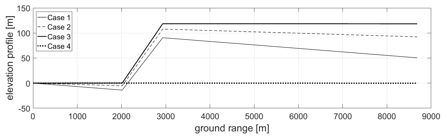
3.2. Sinusoidal DEM
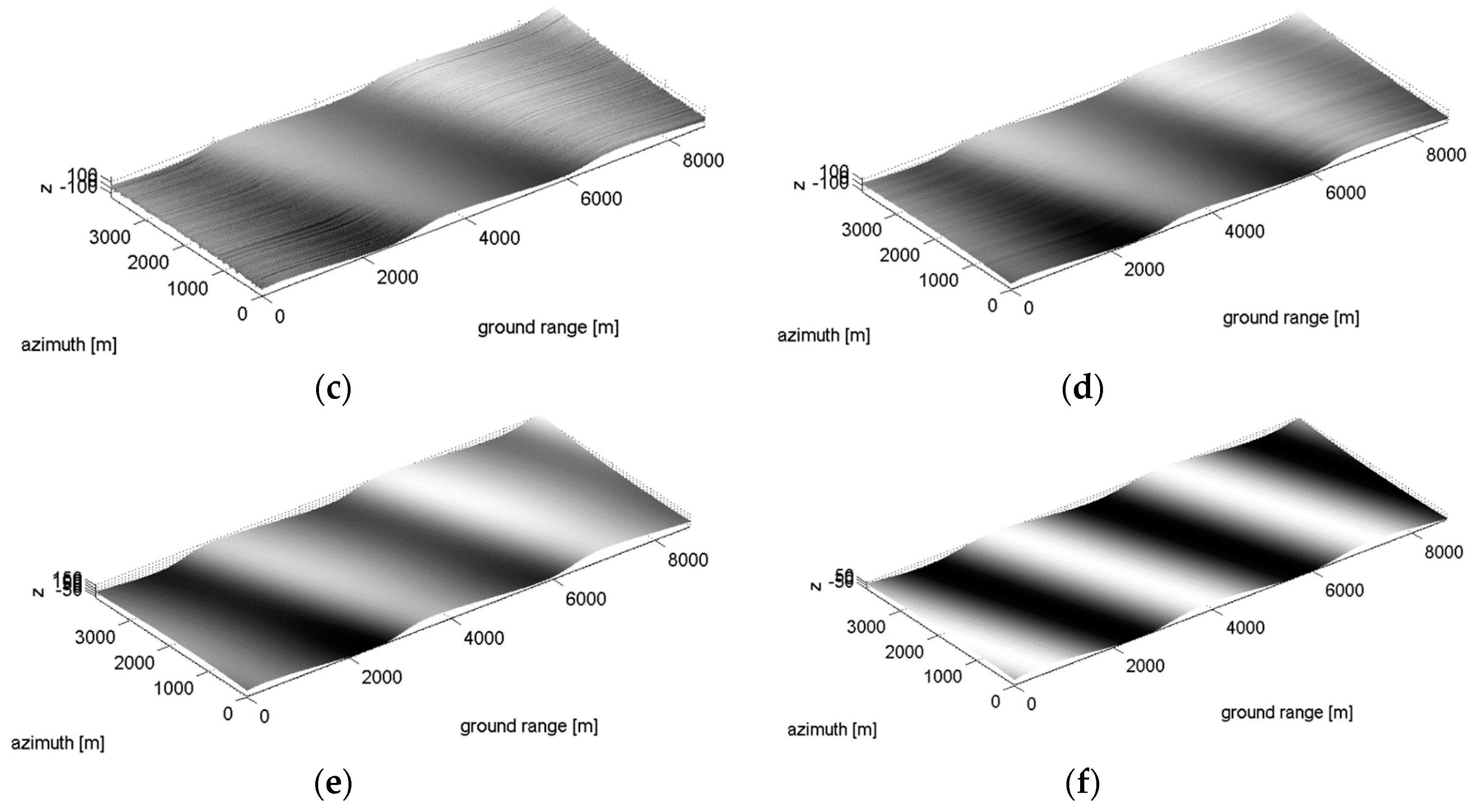
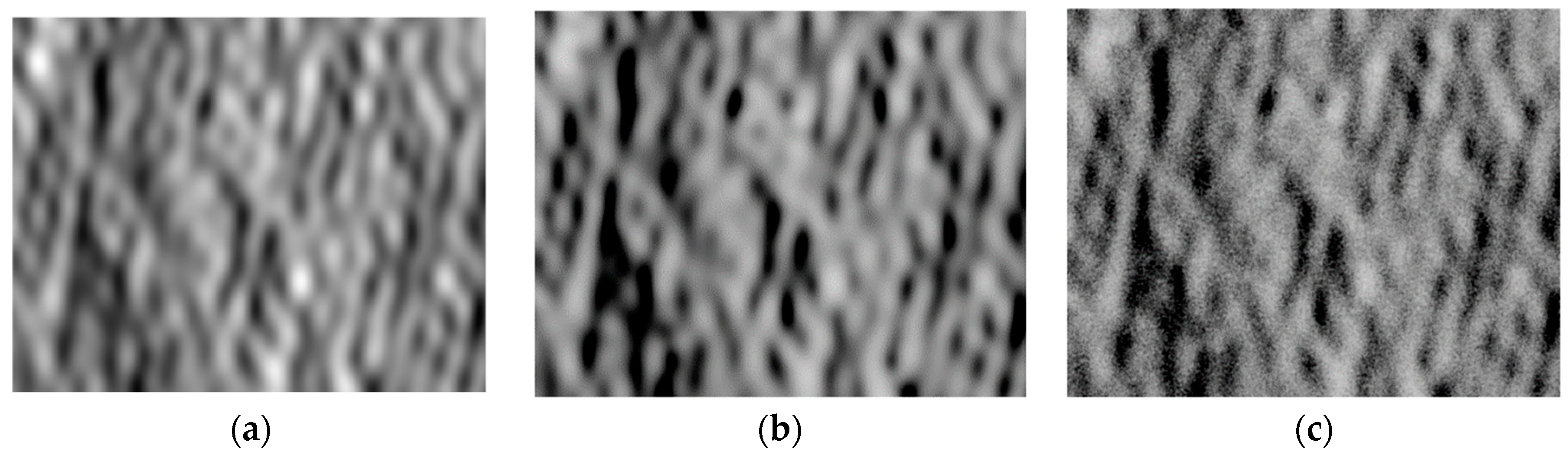
3.3. Fractal DEM
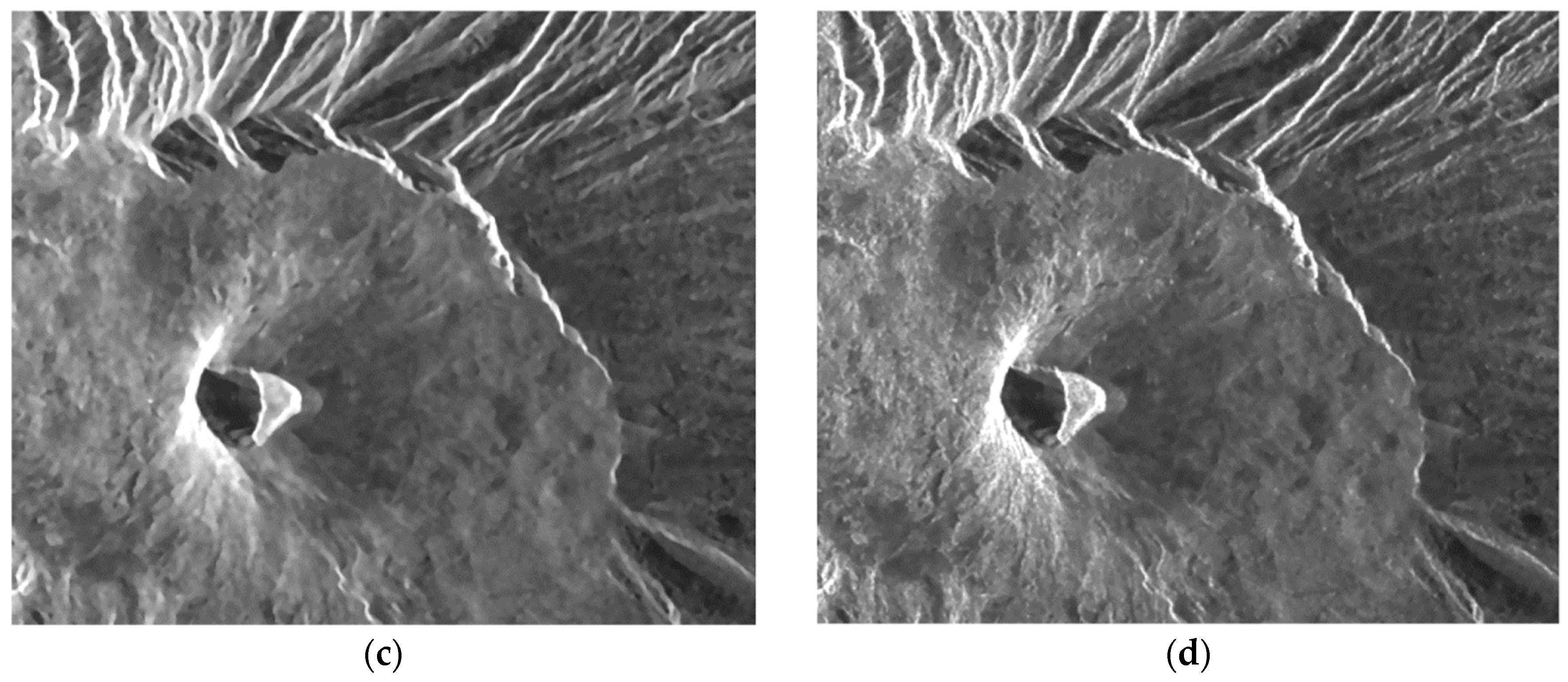
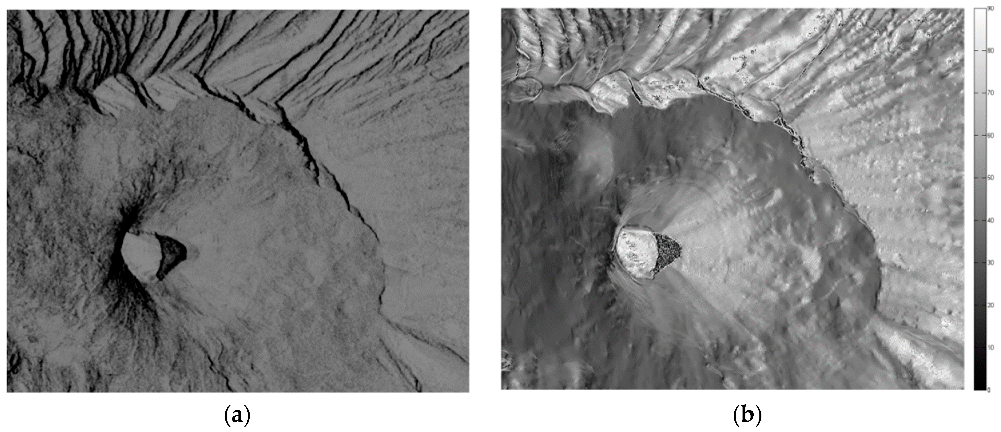
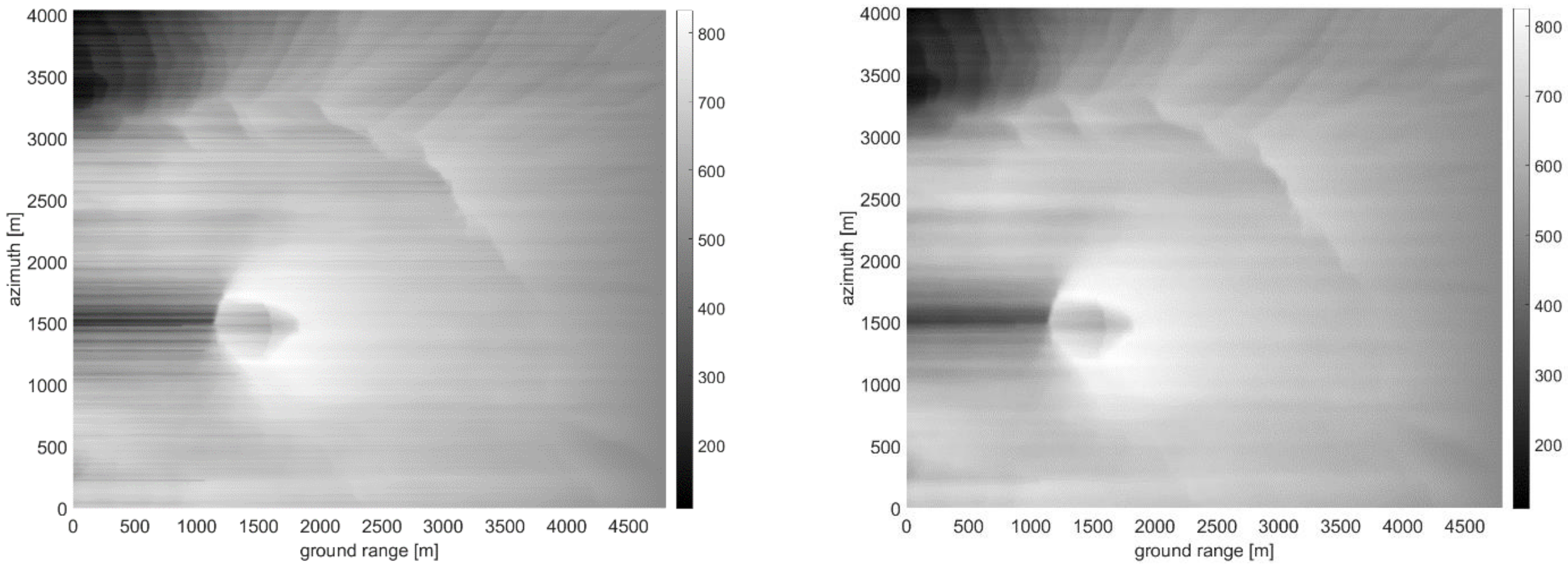
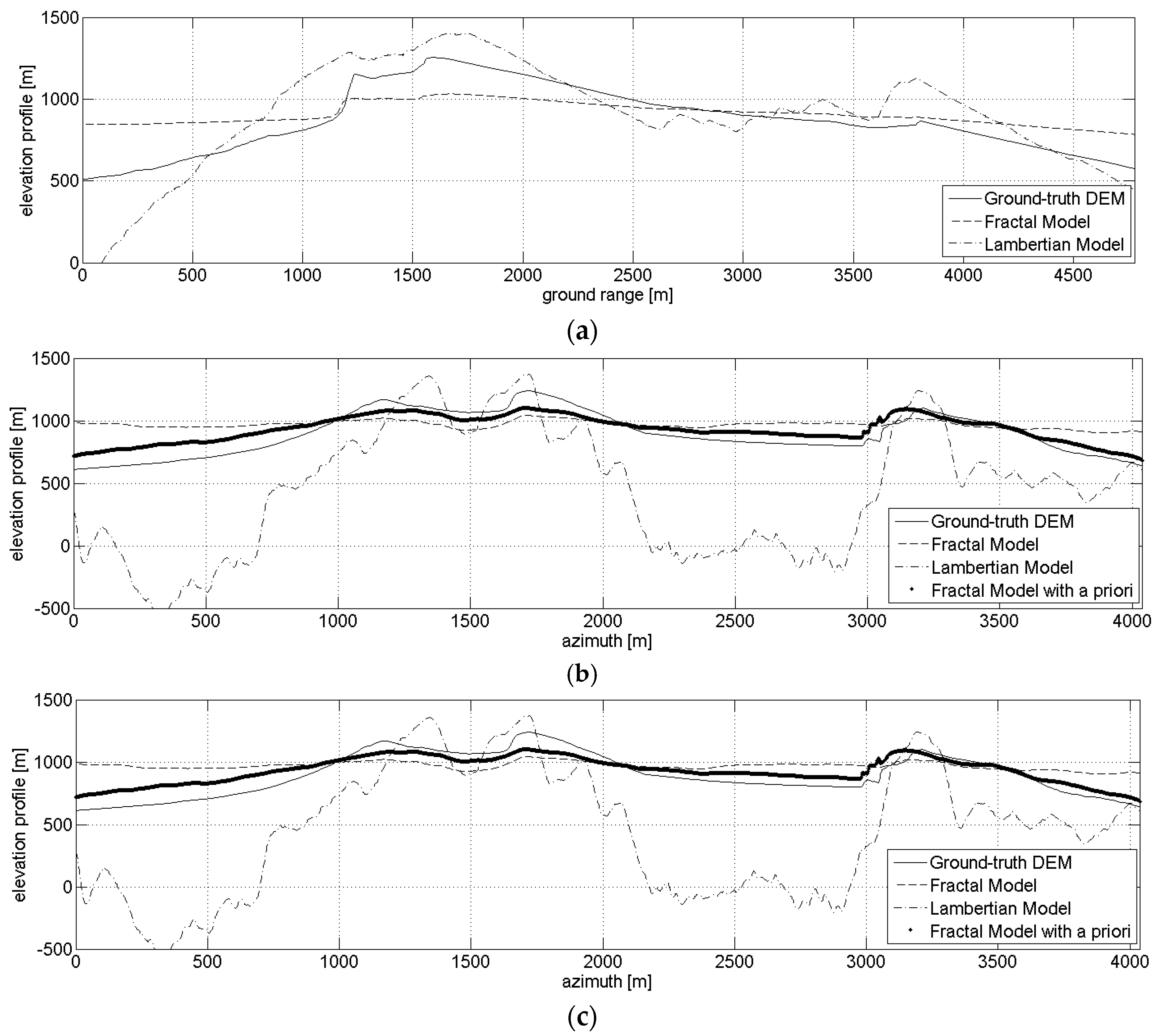
3.4. Actual Case Study
4. Conclusions
Author Contributions
Funding
Conflicts of Interest
Appendix A
References
- Dumitru, C.O.; Datcu, M. Information Content of Very High Resolution SAR Images: Study of Feature Extraction and Imaging Parameters. IEEE Trans. Geosci. Remote Sens. 2013, 51, 4591–4610. [Google Scholar] [CrossRef]
- Grasset, O.; Dougherty, M.K.; Coustenis, A.; Bunce, E.J.; Erd, C.; Titov, D.; Blanc, M.; Coates, A.; Drossart, P.; Fletcher, L.N.; et al. JUpiter ICy moons Explorer (JUICE): An ESA mission to orbit Ganymede and to characterise the Jupiter system. Planet. Space Sci. 2013, 78, 1–21. [Google Scholar] [CrossRef]
- Elachi, C.; Wall, S.; Allison, M.; Anderson, Y.; Boehmer, R.; Callahan, P.; Encrenaz, P.; Flamini, E.; Franceschetti, G.; Gim, Y.; et al. Cassini Radar Views of the Surface of Titan. Science 2005, 308, 970–974. [Google Scholar] [CrossRef] [PubMed]
- Neish, C.D.; Lorenz, R.D.; Kirk, R.L. Radar topography of domes on planetary surfaces. Icarus 2008, 196, 552–564. [Google Scholar] [CrossRef]
- Radebaugh, J.; Lorenz, R.D.; Lunine, J.I.; Wall, S.D.; Boubin, G.; Reffet, E.; Kirk, R.L.; Lopes, R.M.; Stofan, E.R.; Soderblom, L.; et al. Dunes on Titan observed by Cassini Radar. Icarus 2008, 194, 690–703. [Google Scholar] [CrossRef]
- Neish, C.D.; Lorenz, R.D. Elevation distribution of Titan’s craters suggests extensive wetlands. Icarus 2014, 228, 27–34. [Google Scholar] [CrossRef]
- Dhond, U.R.; Aggarwal, J.K. Structure from stereo—A review. IEEE Trans. Syst. Man Cybern. 1989, 19, 1489–1510. [Google Scholar] [CrossRef]
- Dowman, I.; Pu-Huai, C.; Clochez, O.; Saundercock, G. Heighting from stereoscopic ERS-1 data. In Proceedings of the Second ERS-1 Symposium, Hamburg, Germany, 11–14 October 1993; pp. 609–614. [Google Scholar]
- Massonnet, D.; Rabaute, T. Radar interferometry: Limits and potential. IEEE Trans. Geosci. Remote Sens. 1993, 31, 455–464. [Google Scholar] [CrossRef]
- Ostrov, D.N. Boundary Conditions and Fast Algorithms for Surface Reconstructions from Synthetic Aperture Radar Data. IEEE Trans. Geosci. Remote Sens. 1999, 37, 335–346. [Google Scholar] [CrossRef]
- Wildey, R.L. Radarclinometry for the Venus radar mapper. Photogramm. Eng. Remote Sens. 1986, 52, 41–50. [Google Scholar]
- Horn, B.K.P. Obtaining shapes from shading information; MIT Press: Cambridge, UK, 1989. [Google Scholar]
- Brooks, M.J.; Horn, B.K.P. Shape from Shading; MIT Press: Cambridge, UK, 1989. [Google Scholar]
- Paquerault, S.; Maitre, H. A New Method for Backscatter Model Estimation and Elevation Map Computation Using Radarclinometry. EUROPTO-SPIE Int. Soc. Opt. Eng. 1998, 3497. [Google Scholar] [CrossRef]
- Le Hegarat-Mascle, S.; Zribi, M.; Ribous, L. Retrieval of elevation by radarclinometry in arid or semi-arid regions. Int. J. Remote Sens. 2005, 26, 2877–2899. [Google Scholar] [CrossRef]
- Chen, X.; Wang, C.; Zhang, H. DEM Generation Combining SAR Polarimetry and Shape-From-Shading Techniques. IEEE Geosci. Remote Sens. Lett. 2009, 6, 28–32. [Google Scholar] [CrossRef]
- Schuler, D.L.; Lee, J.S.; Grandi, G.D. Measurement of topography using polarimetric SAR images. IEEE Trans. Geosci. Remote Sens. 1996, 34, 1266–1277. [Google Scholar] [CrossRef]
- Markham, K.J.; Morris, W.A. A comparison of radar altimetry and repeat pass interferometry as methods of producing digital terrain elevation models. In Proceedings of the Geoscience and Remote Sensing Symposium, Toronto, Canada, 24–28 June 2002. [Google Scholar]
- Anderson, J.M.M.; Qatshan, A.S.A. Matched filtering-based estimation of ground elevation using laser altimetry. IEEE Trans. Geosci. Remote Sens. 2001, 39, 2168–2175. [Google Scholar] [CrossRef]
- Van Diggelen, J. A photometric investigation of the slopes and the heights of the ranges of hills in the Maria of the moon. Bull. Astron. Inst. Neth. 1951, 11, 283–290. [Google Scholar]
- Wildey, R.L. The surface integral approach to radarclinometry. Earth Moon Planets 1988, 41, 141–153. [Google Scholar] [CrossRef]
- Frankot, R.T.; Chellappa, R. A method for enforcing integrability in shape-from-shading algorithms. IEEE Trans. Pattern Anal. Mach. Intell. 1988, 10, 439–451. [Google Scholar] [CrossRef]
- Guindon, B. Development of a Shape-from-Shading Technique for the Extraction of Topography Models from Individual Spaceborne SAR Images. IEEE Trans. Geosci. Remote Sens. 1990, 28, 654–661. [Google Scholar]
- Bors, A.G.; Hancock, E.R.; Wilson, R.C. Terrain Analysis Using Radar Shape-from-Shading. IEEE Trans. Pattern Anal. Mach. Intell. 2003, 25, 974–992. [Google Scholar] [CrossRef]
- Schuler, D.L.; Lee, J.S.; Kasilingam, D.; Nesti, G. Surface roughness and slope measurements using polarimetric SAR data. IEEE Trans. Geosci. Remote Sens. 2002, 40, 687–698. [Google Scholar] [CrossRef]
- Schuler, D.L.; Ainsworth, T.L.; Lee, J.S. Topographic mapping using polarimetric SAR data. Int. J. Remote Sens. 1998, 19, 141–160. [Google Scholar] [CrossRef]
- Schuler, D.L.; Lee, J.S.; Ainsworth, T.L.; Grunes, M.R. Terrain topography measurement using multipass polarimetric synthetic aperture radar data. Radio Sci. 2000, 35, 813–832. [Google Scholar] [CrossRef]
- Di Martino, G.; Riccio, D.; Zinno, I. SAR Imaging of Fractal Surfaces. IEEE Trans. Geosci. Remote Sens. 2012, 50, 630–644. [Google Scholar] [CrossRef]
- Neish, C.D.; Lorenz, R.D.; Kirk, R.L.; Wye, L.C. Radarclinometry of the sand seas of Africa’s Namibia and Saturn’s moon Titan. Icarus 2010, 208, 385–394. [Google Scholar] [CrossRef]
- Di Martino, G.; Di Simone, A.; Iodice, A.; Riccio, D. Scattering-Based Non-Local Means SAR Despeckling. IEEE Trans. Geosci. Remote Sens. 2016, 54, 3574–3588. [Google Scholar] [CrossRef]
- Di Martino, G.; Di Simone, A.; Iodice, A.; Poggi, G.; Riccio, D.; Verdoliva, L. Scattering-Based SARBM3D. IEEE J. Sel. Top. Appl. Earth Observ. Remote Sens. 2016, 9, 2131–2144. [Google Scholar] [CrossRef]
- Di Martino, G.; Di Simone, A.; Iodice, A.; Riccio, D.; Ruello, G. Non-local means SAR despeckling based on scattering. In Proceedings of the IEEE International Geoscience and Remote Sensing Symposium (IGARSS), Milan, Italy, 26–31 July 2015; pp. 3172–3174. [Google Scholar]
- Frankot, R.T.; Chellappa, R. Estimation of Surface Topography from SAR Imagery Using Shape from Shading Techniques. Artif. Intell. 1990, 43, 271–310. [Google Scholar] [CrossRef]
- Mandelbrot, B. The Fractal Geometry of Nature; Freeman: New York, NY, USA, 1983. [Google Scholar]
- Falconer, K. Fractal Geometry; John Wiley: Chichester, UK, 1990. [Google Scholar]
- Feder, J.S. Fractals; Plenum Press: New York, NY, USA, 1988. [Google Scholar]
- Shepard, M.K.; Campbell, B.A.; Bulmer, M.H.; Farr, T.G.; Gaddis, L.R. The roughness of natural terrain: A planetary and remote sensing perspective. J. Geophys. Res. 2001, 106, 32777–32795. [Google Scholar] [CrossRef]
- Campbell, B.A. Scale-dependent surface roughness behavior and its impact on empirical models for radar backscatter. IEEE Trans. Geosci. Remote Sens. 2009, 47, 3480–3488. [Google Scholar] [CrossRef]
- Pentland, A.P. Fractal-Based Description of Natural Scenes. IEEE Trans. Pattern Anal. Mach. Intell. 1984, PAMI-6, 661–674. [Google Scholar] [CrossRef]
- Franceschetti, G.; Riccio, D. Scattering, Natural Surfaces and Fractals; Academic Press: Burlington, MA, USA, 2007. [Google Scholar]
- Franceschetti, G.; Iodice, A.; Maddaluno, S.; Riccio, D. A Fractal-Based Theoretical Framework for Retrieval of Surface Parameters from Electromagnetic Backscattering Data. IEEE Trans. Geosci. Remote Sens. 2000, 38, 641–650. [Google Scholar] [CrossRef]
- Franceschetti, G.; Lanari, R. Synthetic Aperture Radar (SAR) Processing; CRC Press: New York, NY, USA, 1999. [Google Scholar]
- Di Martino, G.; Iodice, A.; Riccio, D.; Ruello, G.; Zinno, I. Angle Independence Properties of Fractal Dimension Maps Estimated from SAR Data. IEEE J. Sel. Top. Appl. Earth Observ. Remote Sens. 2013, 6, 1242–1253. [Google Scholar] [CrossRef]
- Ulander, L.M.H. Radiometric Slope Correction of Synthetic-Aperture Radar images. IEEE Trans. Geosci. Remote Sens. 1996, 34, 1115–1122. [Google Scholar] [CrossRef]
- Zhang, Q.; Yuan, Q.; Li, J.; Yang, Z.; Ma, X. Learning a Dilated Residual Network for SAR Image Despeckling. Remote Sens. 2018, 10, 196. [Google Scholar] [CrossRef]
- Wang, P.; Zhang, H.; Patel, V.M. SAR Image Despeckling Using a Convolutional Neural Network. IEEE Signal Process. Lett. 2018, 24, 1763–1767. [Google Scholar] [CrossRef]
- Ma, X.; Wu, P.; Wu, Y.; Shen, H. A Review on Recent Developments in Fully Polarimetric SAR Image Despeckling. IEEE J. Sel. Top. Appl. Earth Observ. Remote Sens. 2018, 11, 743–758. [Google Scholar] [CrossRef]
- Deledalle, C.-A.; Denis, L.; Tupin, F. Iterative weighted maximum likelihood denoising with probabilistic patch-based weights. IEEE Trans. Image Process. 2009, 18, 2661–2672. [Google Scholar] [CrossRef] [PubMed]
- Parrilli, S.; Poderico, M.; Angelino, C.V.; Verdoliva, L. A nonlocal SAR image denoising algorithm based on LLMMSE wavelet shrinkage. IEEE Trans. Geosci. Remote Sens. 2012, 50, 606–616. [Google Scholar] [CrossRef]
- Di Simone, A. Sensitivity Analysis of the Scattering-Based SARBM3D Despeckling Algorithm. Sensors 2016, 16, 971. [Google Scholar] [CrossRef] [PubMed]
- Di Martino, G.; Di Simone, A.; Iodice, A.; Riccio, D. Sensitivity Analysis of a Scattering-Based Nonlocal Means Despeckling Algorithm. Eur. J. Remote Sens. 2017, 50, 87–97. [Google Scholar]
- Franceschetti, G.; Migliaccio, M.; Riccio, D.; Schirinzi, G. SARAS: A SAR raw signal simulator. IEEE Trans. Geosci. Remote Sens. 1992, 30, 110–123. [Google Scholar] [CrossRef]
- Di Martino, G.; Poderico, M.; Poggi, G.; Riccio, D.; Verdoliva, L. Benchmarking Framework for SAR Despeckling. IEEE Trans. Geosci. Remote Sens. 2014, 52, 1596–1615. [Google Scholar] [CrossRef]
- Ruello, G.; Blanco, P.; Iodice, A.; Mallorqui, J.J.; Riccio, D.; Broquetas, A.; Franceschetti, G. Synthesis, construction and validation of a fractal surface. IEEE Trans. Geosci. Remote Sens. 2006, 44, 1403–1412. [Google Scholar]
- Berry, M.V.; Lewis, Z.V. On the Weierstrass-Mandelbrot fractal function. Proc. R. Soc. Lond. A Math. Phys. Sci. 1980, 370, 459–484. [Google Scholar] [CrossRef]
- Tsang, L.; Kong, J.A.; Ding, K. Scattering of Electromagnetic Waves, Theories and Applications; John Wiley: New York, NY, USA, 2000. [Google Scholar]
- Di Martino, G.; Di Simone, A.; Iodice, A.; Riccio, D.; Ruello, G. Estimation of the local incidence angle map from a single SAR image. In Proceedings of the ESA Living Planet Symposium 2016, ESA SP 740, Prague, Czech Republic, 9–13 May 2016. [Google Scholar]
- Di Martino, G.; Poggi, G.; Riccio, D.; Verdoliva, L. Effects of despeckling on the estimation of fractal dimension from SAR images. In Proceedings of the Geoscience and Remote Sensing Symposium (IGARSS), Melbourne, Australia, 21–26 July 2013. [Google Scholar]


| Error Magnitude | Elevation (m) | Range Slope (°) | Azimuth Slope (°) | ||||||||
|---|---|---|---|---|---|---|---|---|---|---|---|
| Median | Mean | Std dev | Median | Mean | Std dev | Median | Mean | Std dev | |||
| Before azimuth filtering | Fractal Model | 34.1 | 38.5 | 26.8 | 1.40 | 1.41 | 1.00 | 1.67 | 1.79 | 1.16 | |
| Lambertian Model | 132.9 | 150.0 | 106.1 | 10.20 | 10.46 | 5.94 | 3.73 | 5.54 | 5.08 | ||
| After azimuth filtering | Unknown starting points | Fractal Model | 33.9 | 38.2 | 26.7 | 1.41 | 1.41 | 0.99 | 1.67 | 1.65 | 0.64 |
| Lambertian Model | 132.5 | 149.0 | 105.0 | 10.07 | 10.35 | 5.89 | 2.36 | 4.66 | 4.66 | ||
| Known starting points | Fractal Model | 27.6 | 28.0 | 17.2 | 1.42 | 1.41 | 0.99 | 0.33 | 0.48 | 0.43 | |
| Lambertian Model | 124.5 | 137.2 | 94.5 | 10.07 | 10.35 | 5.89 | 0.87 | 3.21 | 4.50 | ||
| Error Magnitude | Elevation (m) | Range Slope (°) | Azimuth Slope (°) | ||||||||
|---|---|---|---|---|---|---|---|---|---|---|---|
| Median | Mean | Std dev | Median | Mean | Std dev | Median | Mean | Std dev | |||
| Before azimuth filtering | Fractal Model | 30.0 | 35.3 | 26.3 | 2.78 | 4.23 | 4.78 | 74.46 | 63.27 | 25.34 | |
| Lambertian Model | 112.1 | 129.7 | 94.6 | 12.22 | 13.43 | 10.45 | 84.53 | 76.33 | 19.37 | ||
| After azimuth filtering | Unknown starting points | Fractal Model | 29.2 | 33.7 | 24.1 | 2.36 | 3.67 | 4.50 | 9.70 | 14.00 | 12.90 |
| Lambertian Model | 110.4 | 124.7 | 88.1 | 9.56 | 12.42 | 10.71 | 21.02 | 25.39 | 20.17 | ||
| Known starting points | Fractal Model | 23.5 | 25.2 | 16.9 | 2.36 | 3.67 | 4.50 | 9.60 | 13.86 | 12.97 | |
| Lambertian Model | 101.2 | 112.4 | 77.6 | 9.57 | 12.42 | 10.71 | 28.53 | 31.54 | 23.18 | ||
| Error Magnitude | Elevation (m) | Range Slope (°) | Azimuth Slope (°) | ||||||||
|---|---|---|---|---|---|---|---|---|---|---|---|
| Median | Mean | Std dev | Median | Mean | Std dev | Median | Mean | Std dev | |||
| Before azimuth filtering—Unknown starting points—Fractal Model | 19.6 | 22.3 | 15.9 | 0.59 | 0.75 | 0.68 | 2.97 | 3.61 | 2.98 | ||
| After azimuth filtering | Unknown starting points | Fractal Model | 19.7 | 22.3 | 15.8 | 0.61 | 0.76 | 0.69 | 2.85 | 3.48 | 2.86 |
| Lambertian Model | 38.9 | 51.7 | 46.8 | 3.42 | 4.09 | 3.47 | 8.81 | 10.78 | 8.76 | ||
| Known starting points | Fractal Model | 17.4 | 19.9 | 14.1 | 0.61 | 0.76 | 0.69 | 2.03 | 2.79 | 2.57 | |
| Lambertian Model | 39.0 | 51.8 | 45.8 | 3.42 | 4.09 | 3.47 | 7.97 | 10.02 | 8.43 | ||
| Error Magnitude | Elevation (m) | Range Slope (°) | Azimuth Slope (°) | |||||||
|---|---|---|---|---|---|---|---|---|---|---|
| Median | Mean | Std dev | Median | Mean | Std dev | Median | Mean | Std dev | ||
| Before azimuth filtering | Fractal Model | 16.1 | 20.8 | 18.0 | 4.32 | 5.40 | 5.18 | 74.49 | 65.95 | 21.83 |
| Lambertian Model | 33.6 | 45.6 | 42.4 | 12.21 | 13.51 | 10.39 | 83.58 | 77.13 | 17.15 | |
| After azimuth filtering | Fractal Model | 17.4 | 19.7 | 14.0 | 2.93 | 4.18 | 4.07 | 7.19 | 9.28 | 7.92 |
| Lambertian Model | 27.7 | 38.0 | 35.3 | 8.01 | 10.71 | 9.37 | 18.37 | 21.31 | 15.70 | |
| Error Magnitude | Elevation (m) | Range Slope (°) | Azimuth Slope (°) | |||||||
|---|---|---|---|---|---|---|---|---|---|---|
| Median | Mean | Std dev | Median | Mean | Std dev | Median | Mean | Std dev | ||
| Before azimuth filtering | Fractal Model | 17.3 | 19.8 | 14.7 | 0.79 | 1.00 | 0.86 | 21.17 | 24.09 | 17.26 |
| Lambertian Model | 28.7 | 39.0 | 36.1 | 2.93 | 3.56 | 2.98 | 47.23 | 42.67 | 23.08 | |
| After azimuth filtering | Fractal Model | 17.6 | 19.8 | 14.3 | 0.71 | 0.89 | 0.75 | 3.43 | 4.10 | 3.76 |
| Lambertian Model | 27.9 | 38.0 | 35.4 | 2.71 | 3.30 | 2.78 | 8.59 | 10.86 | 9.14 | |
| Error Magnitude | Elevation (m) | Range Slope (°) | Azimuth Slope (°) | ||||||||
|---|---|---|---|---|---|---|---|---|---|---|---|
| Median | Mean | Std dev | Median | Mean | Std dev | Median | Mean | Std dev | |||
| Before azimuth filtering | Fractal Model | 140.7 | 163.9 | 118.4 | 9.32 | 11.20 | 9.40 | 21.31 | 27.10 | 22.03 | |
| Lambertian Model | 318.8 | 501.1 | 492.0 | 24.43 | 29.61 | 21.20 | 83.39 | 79.50 | 25.65 | ||
| After azimuth filtering | Unknown starting points | Fractal Model | 140.7 | 163.9 | 118.3 | 9.38 | 11.33 | 9.51 | 12.20 | 15.08 | 12.69 |
| Lambertian Model | 312.0 | 490.8 | 481.8 | 28.55 | 33.86 | 21.73 | 60.78 | 56.79 | 27.99 | ||
| Known starting points | Fractal Model | 98.4 | 124.4 | 102.4 | 9.38 | 11.33 | 9.51 | 9.22 | 13.80 | 15.20 | |
| Lambertian Model | 307.7 | 492.3 | 498.6 | 28.55 | 33.86 | 21.73 | 60.07 | 56.13 | 28.17 | ||
© 2018 by the authors. Licensee MDPI, Basel, Switzerland. This article is an open access article distributed under the terms and conditions of the Creative Commons Attribution (CC BY) license (http://creativecommons.org/licenses/by/4.0/).
Share and Cite
Di Martino, G.; Di Simone, A.; Riccio, D. Fractal-Based Local Range Slope Estimation from Single SAR Image with Applications to SAR Despeckling and Topographic Mapping. Remote Sens. 2018, 10, 1294. https://doi.org/10.3390/rs10081294
Di Martino G, Di Simone A, Riccio D. Fractal-Based Local Range Slope Estimation from Single SAR Image with Applications to SAR Despeckling and Topographic Mapping. Remote Sensing. 2018; 10(8):1294. https://doi.org/10.3390/rs10081294
Chicago/Turabian StyleDi Martino, Gerardo, Alessio Di Simone, and Daniele Riccio. 2018. "Fractal-Based Local Range Slope Estimation from Single SAR Image with Applications to SAR Despeckling and Topographic Mapping" Remote Sensing 10, no. 8: 1294. https://doi.org/10.3390/rs10081294
APA StyleDi Martino, G., Di Simone, A., & Riccio, D. (2018). Fractal-Based Local Range Slope Estimation from Single SAR Image with Applications to SAR Despeckling and Topographic Mapping. Remote Sensing, 10(8), 1294. https://doi.org/10.3390/rs10081294