The main finding of our study is that no universally valid combination of inversion model, , and estimation algorithm, and segment size is available to obtain accurate estimates of PAI and WAI for all leaf-on and leaf-off forest canopies. Both the factors of inversion model, , , , , , and segment size are contributed to the differences between the PAI and WAI estimated from the seven inversion models. The performance of the combination of inversion model, , and , estimation algorithm, and segment size to estimate the PAI and WAI of leaf-on and leaf-off forest scenes is the function of the inversion model, , and estimation algorithm, segment size, PAI, WAI, tree species composition, and plant functional types.
5.1. Reason for Differences between , PAI, and WAI Estimates Estimated from the Seven Inversion Models with or without Consideration of , , , , and
Since
,
,
,
,
, and
varied obviously with zenith angles in the range of 0–90° (
Figure 3,
Figure 5 and
Figure 6). The trend in the variations of
,
,
, and
with zenith angles in the range of 0–90° did not comply with the trend in the variations of
and
in the same zenith angle range (
Figure 3,
Figure 5 and
Figure 6). However, different zenith angle ranges were used by the seven inversion models to estimate the PAI and WAI of leaf-on and leaf-off forest scenes. Therefore, both the inversion model,
,
,
,
and
estimation algorithm, and segment size are the factors that contributed to the differences between the PAI or WAI estimated from the seven inversion models. That’s because the
,
,
,
,
,
,
,
,
,
,
,
,
,
, and
that were used in the PAI and WAI estimation for the seven inversion models are obviously different between each other.
Amongst the five factors of the inversion model,
and
,
,
and
estimation algorithm, and segment size, the PAI and WAI estimation was less affected by
and
; by contrast, the PAI and WAI estimation was largely affected by other factors (
Figure 8,
Figure 9 and
Figure 11,
Table 2,
Table 3,
Table 4,
Table A1 and
Table A2) (
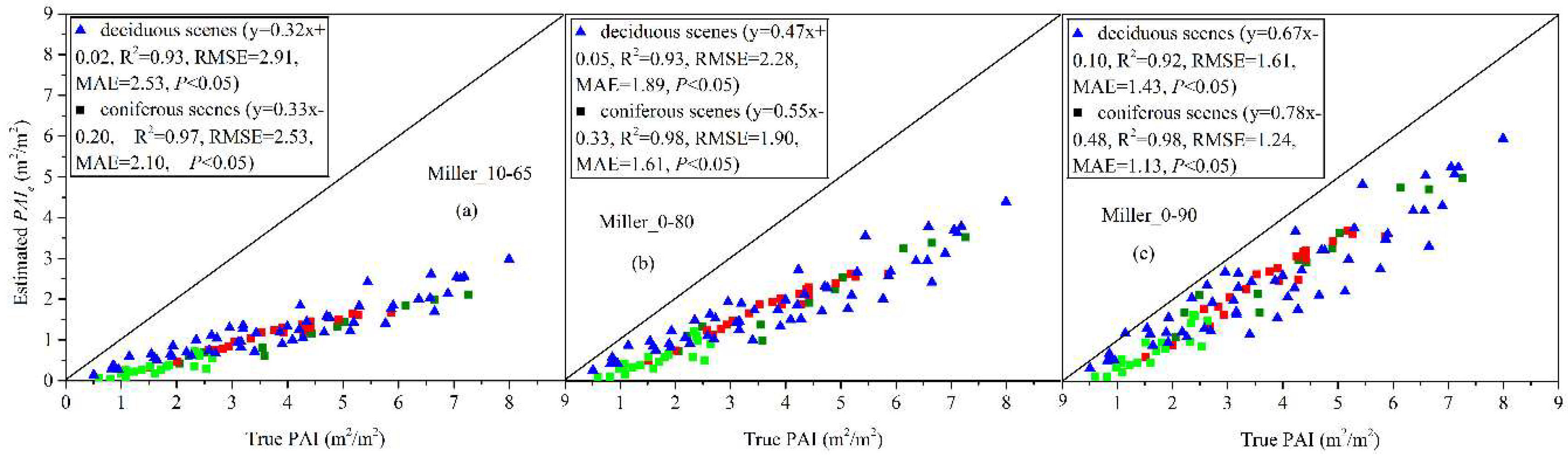
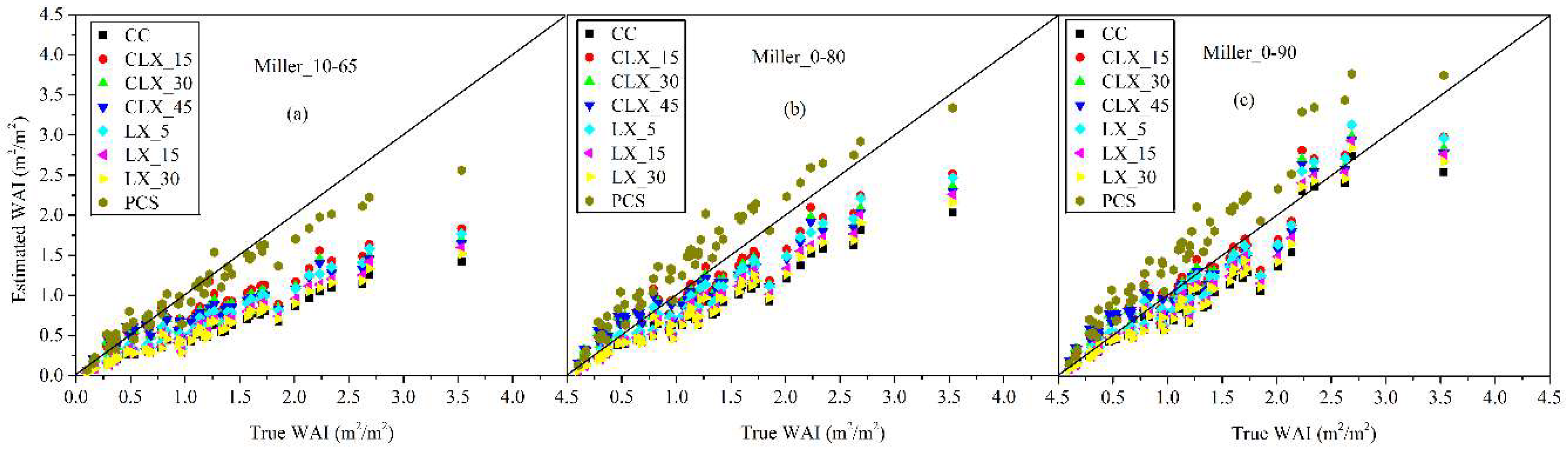
Appendix C.1). The largest variation in proportion between the
, PAI,
, and WAI estimated from any two inversion models amongst the seven inversion models with or without consideration of
,
,
,
, and
at the leaf-on and leaf-off scenes is that derived from Miller_10-65 and Miller_0-90 (Equations (3) and (5)) without consideration of
,
, and
, but with consideration of
and
(
Figure 8,
Figure 9 and
Figure 11,
Table 2,
Table 3,
Table 4,
Table A1 and
Table A2). The mean
and
estimates derived from Miler_0-90 are approximately two times the estimates derived from Miller_10-65 (
Table 2). This result means that the inversion model contributed more to the variations between the results of the seven inversion models as the variations in proportion tended to decrease if
and
were considered in the
, PAI,
, and WAI estimation (
Table 2,
Table 4,
Table A1 and
Table A2). The zenith angle ranges covered by the two inversion models of Miller_10-65 and Miller_0-90 and the processing solution of the null gap fraction measurements can explain the large differences between the mean
or
estimates of the two inversion models. The reason is that both the logarithm of the mean
and
, and the weight (
) tended to increase with zenith angles in the range of 0–90° (
Figure 3). Further, the defined PAI and WAI of 10 for the null gap fraction measurements at the zenith angles close to the horizon are usually larger than the estimates derived using Equation (4) based on the mean
and
collected at the zenith angle range of 10–65°.
Compared with two inversion models, namely, Miller_10-65, and Miller_0-90, the variations in proportion between the mean
or
estimates of any other two inversion models estimated without consideration of
and
are relatively small (
Table 2,
Table 3 and
Table 4). The variations of the
and
in the zenith angle range of 0–90° at the leaf-on and leaf-off forest canopy are specific to sites, species, and estimation algorithms [
10,
17,
41,
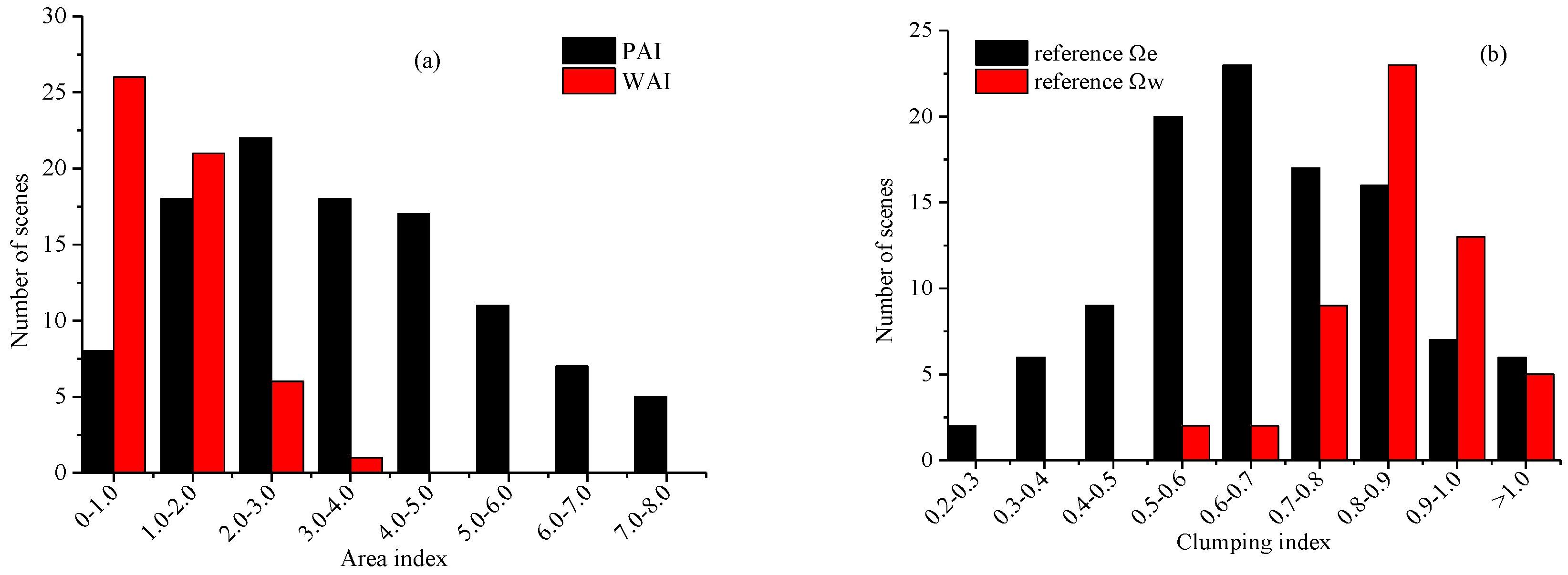
61]. Chen et al. [
61] reported that the
of most natural forest stands range from 0.50 to 0.75. Similarly, the
of the coniferous forest canopy is also specific to sites and tree species, and previous studies reported that
usually ranges from 1.20 to 2.08 [
10,
22,
47]. Therefore, amongst the four factors of the inversion model,
,
and
estimation algorithm, and segment size, the dominant factor that contributed more to the differences between the PAI or WAI estimated from the seven inversion models except Miller_10-65 considering
,
,
,
, and
is the function of the inversion model,
,
and
estimation algorithm, segment size, and tree species composition, and the structural characteristics of the forest canopy.
The differences between the mean
or
results of the two inversion models covered with the same zenith angle ranges, such as Miller_0-90 and DHP_0-90, and DHP_0-81 and DHP_0-90, are mainly deduced from the differences between the gap fraction and weight calculation methods of the two inversion models (
Table 2 and
Table 3). For these inversion models covered with different zenith angle ranges, such as Miller_0-80 and Miller_0-90, and Miller_0-80 and DHP_0-90, all the three aspects of the inversion model, including zenith angle range, gap fraction, and weight calculation methods, are the main sources of differences between the
or
estimates of the different inversion models (
Figure 4,
Table 2 and
Table 3).
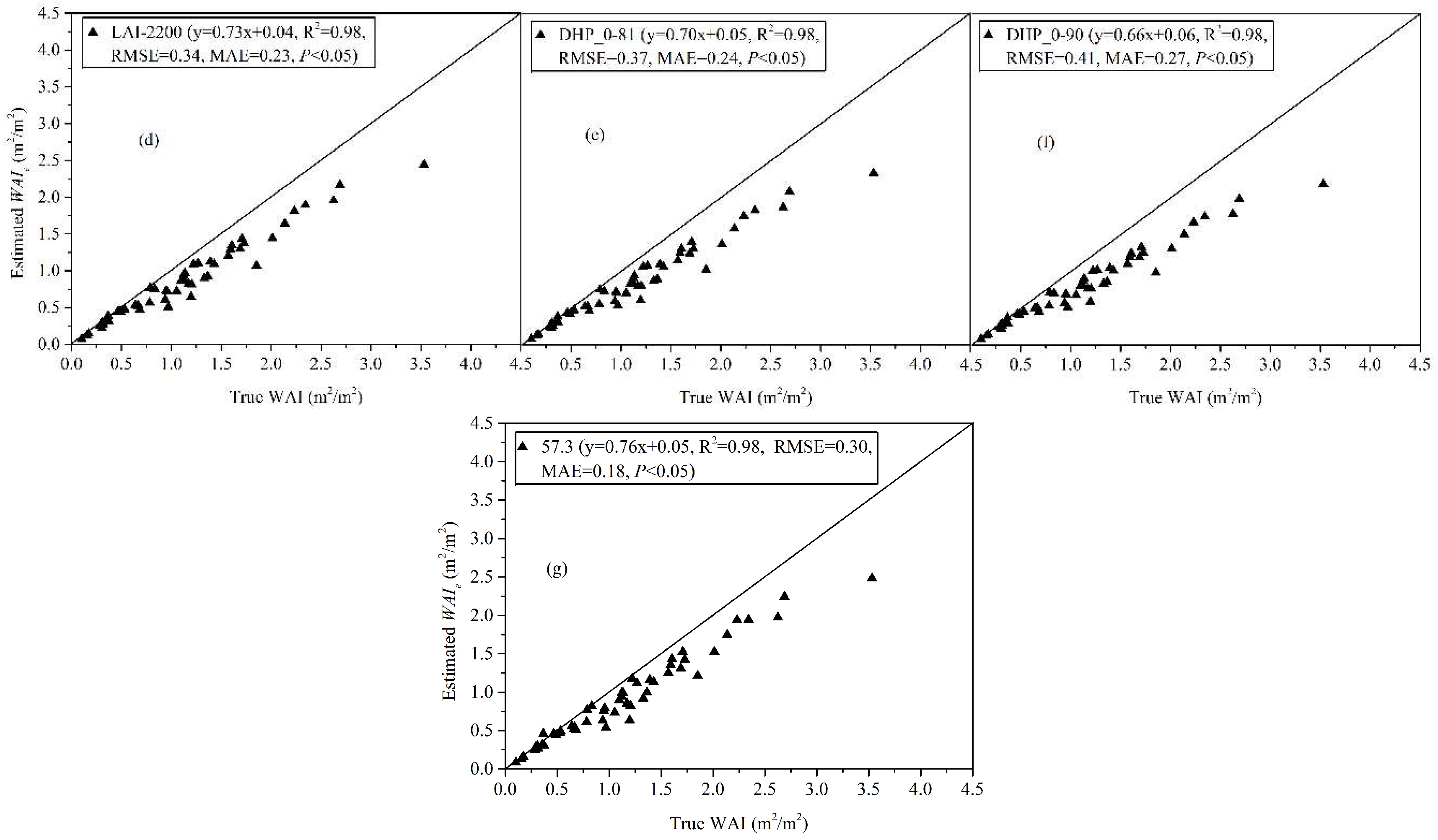
5.2. Can PAI or WAI be Estimated Accurately from the Currently Available Inversion Models without Field Measurements of and of Forest Canopy
To address the challenge of measuring the
and
of the leaf-on and leaf-off forest canopy, the 57.3 inversion model was recommended by many previous studies to derive the PAI and LAI of vegetation canopy [
18,
22,
45,
62]. Previous studies showed that this inversion model is a good choice to avoid the error source of
and
in the PAI and WAI estimation of vegetation canopy [
18,
45,
62]; this conclusion was also confirmed in the present study (
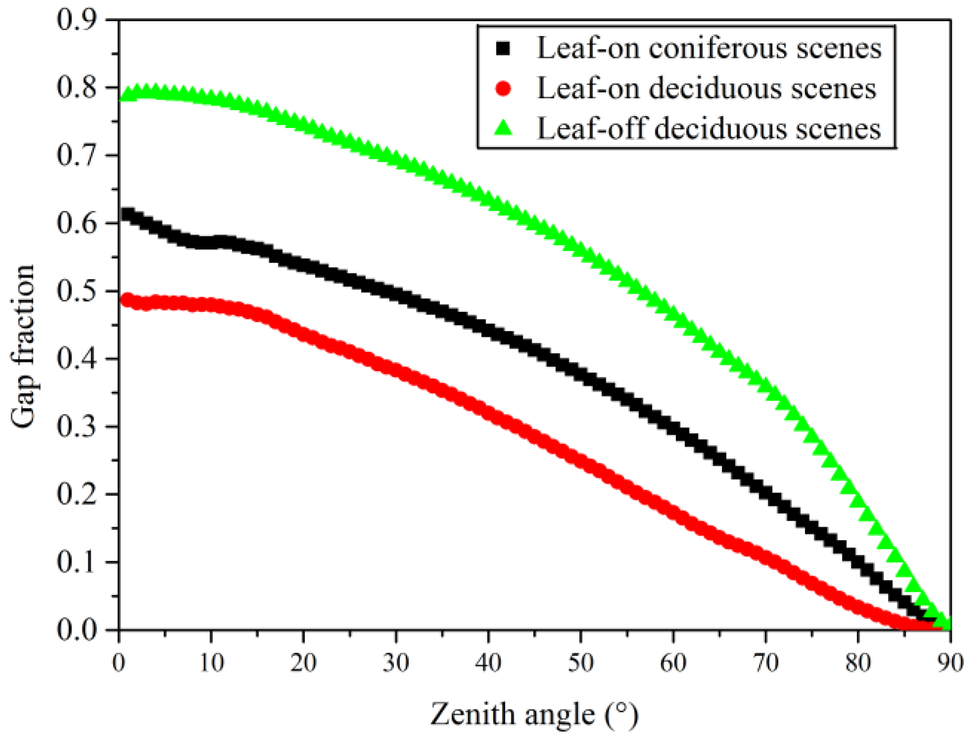
Figure 5 and
Table 2 and
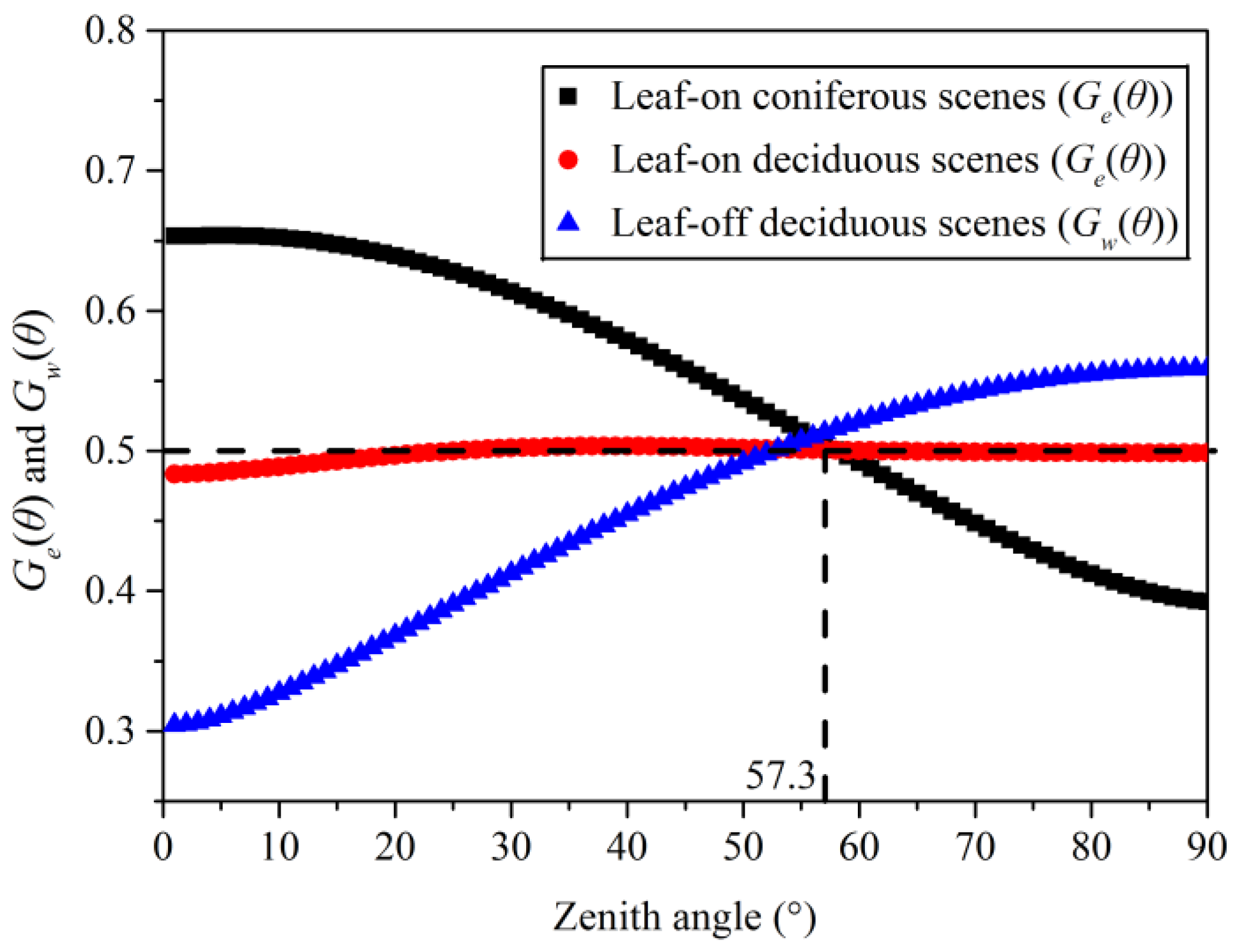
Table 3). The merit of the 57.3 inversion model is that the
and
of leaf-on and leaf-off forest canopy were approximately intersected at the zenith angle near 57.3° (1 radian) and are equal to about 0.5 at this zenith angle [
7,
15,
45,
63]; this conclusion was also confirmed in the present study at the leaf-on and leaf-off scenes with three typical and contrasting types of
and
(
Figure 5).
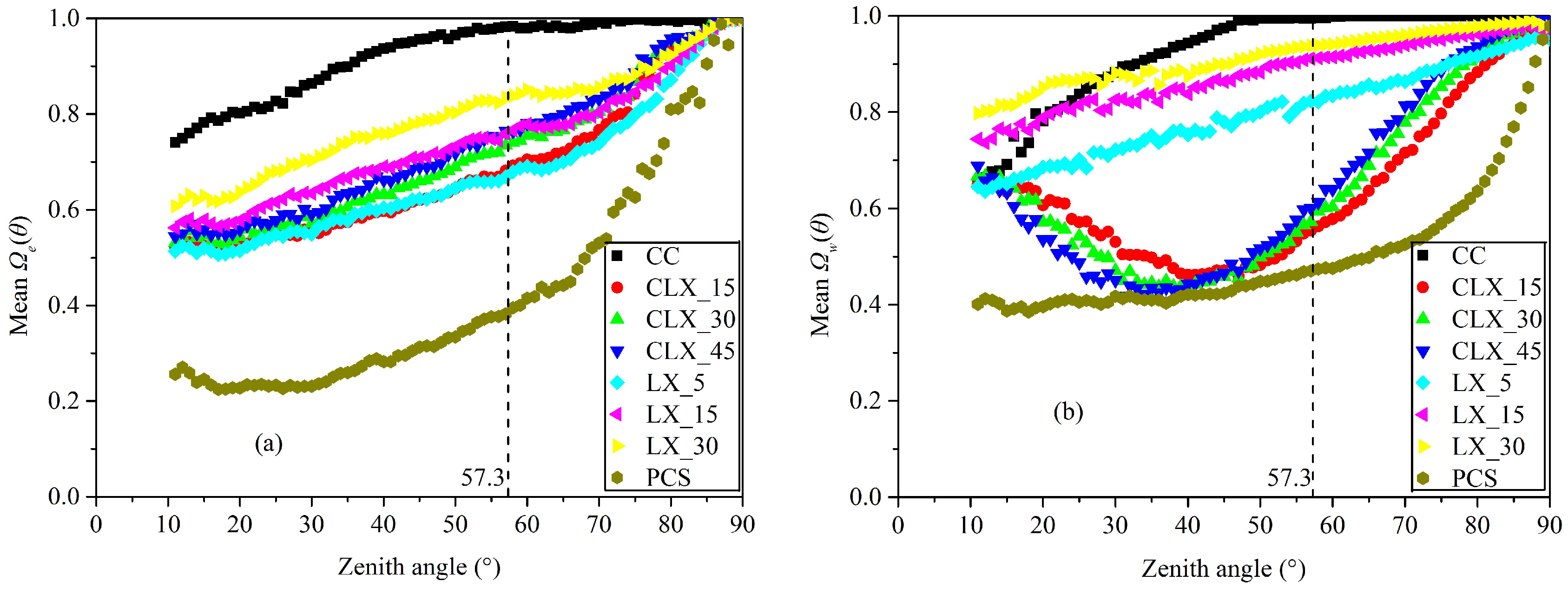
Since the
and
varied obviously with zenith angles in the range of 0–90° (
Figure 5), the
and
measurements would be the critical input parameters for the seven inversion models except 57.3 in the PAI and WAI estimation of leaf-on and leaf-off scenes. A sign of the important role of
and
in the PAI and WAI estimation is that large differences were found between the
or
estimates derived from Miller_10-65 estimated with or without consideration of
and
(
Table 2 and
Table 3). The large differences indicate that it is inappropriate to assume that
and
are equal to 0.5 at all zenith angles in the PAI and WAI estimation. However, the minor differences in proportion between the
or
estimated using the inversion models of Miller_0-80, LAI-2200, DHP_0-81, and DHP_0-90 with or without consideration of
and
are small (below <4%) (
Table 2 and
Table 3), showing that the error source of
and
was largely reduced in the
and
estimation. The zenith angle ranges covered by the four inversion models is the reason for the reduction of the error source of
and
in the
and
estimation. As inferred from Equation (4) that the PAI and WAI are linearly related to the
and
, respectively, therefore, the PAI and WAI estimation errors are equivalent in proportion to the
and
errors. Therefore, the trade-off between the
and
overestimation or underestimation caused by the underestimation or overestimation of
and
at zenith angles less than near 57°, and the opposite trend of the
, and
underestimation or overestimation caused by the overestimation or underestimation of
and
at zenith angles greater than near 57° are the reason for the removal of the error source of
and
in the
and
estimation for the four inversion models (
Figure 5,
Table 2 and
Table 3). The larger values of the logarithm of the mean
and
, and
at the zenith angle range of 57–90° compared with those at the zenith angle range of 0–57° can explain why a narrow zenith angle range of the former zenith angle range is enough to trade off the
and
underestimation or overestimation caused by the error source of
and
at the latter zenith angle range. Therefore, we can conclude that the impact of
and
on the
,
, PAI, and WAI estimation of leaf-on and leaf-off forest canopy can be reduced to a low level (4%) by selecting appropriate inversion models such as Miller_0-80, LAI-2200, DHP_0-81, DHP_0-90, and 57.3.
5.3. Can the and of Leaf-on and Leaf-off Forest Canopy be Effectively Estimated based on the DHP Images Using the Currently Available Algorithms
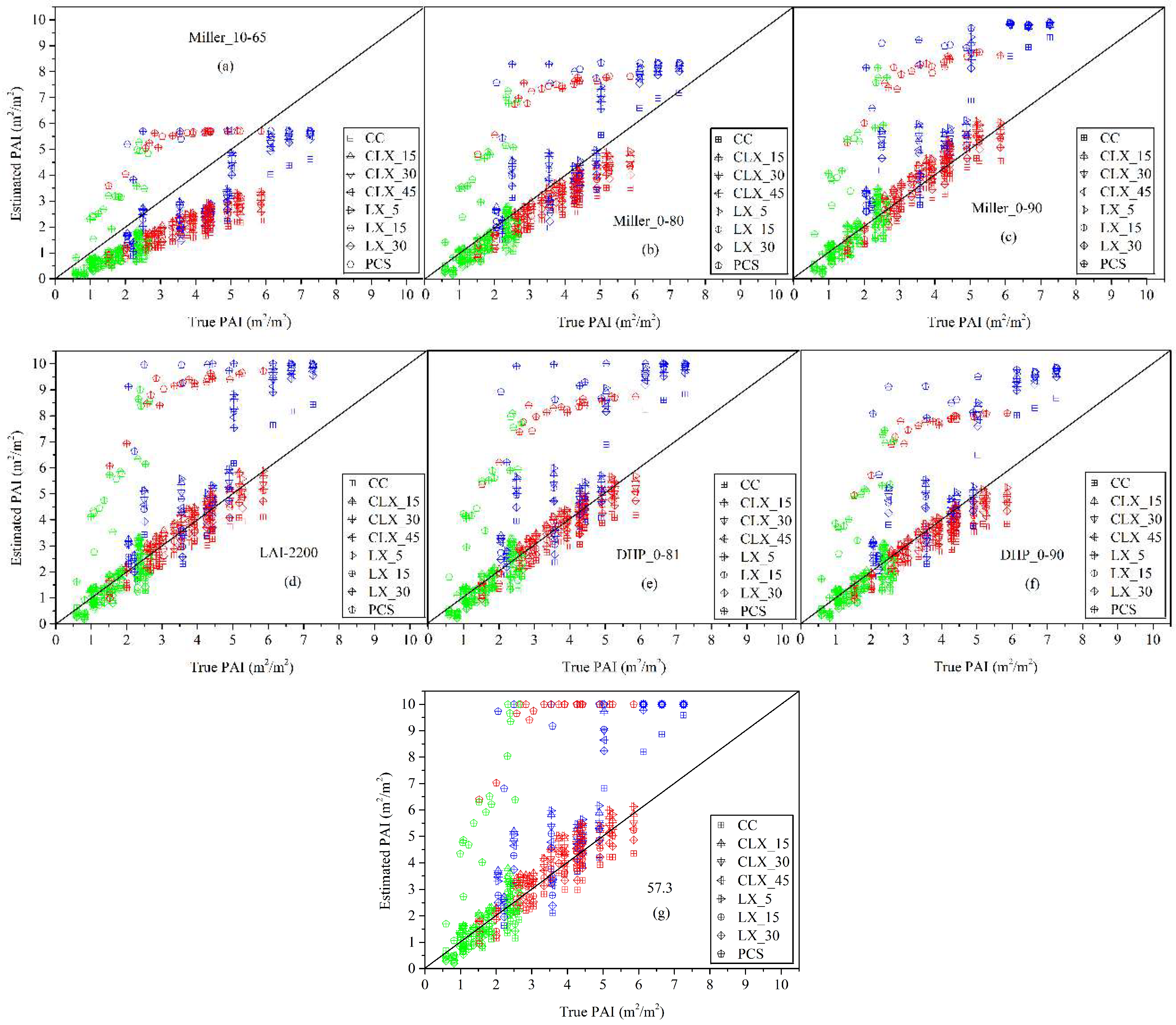
The PAI and WAI underestimation of the seven inversion models were largely reduced or removed if the
,
, and
were considered in the PAI and WAI estimation of leaf-on and leaf-off scenes, except the combinations of inversion model,
,
, and
estimation algorithm and segment size with PCS (
Figure 7,
Figure 8,
Figure 9,
Figure 10 and
Figure 11,
Table A1 and
Table A2). Therefore, we can conclude that the clumping effect of the canopy element and woody component of the forest canopy was the main reason for the severe PAI and WAI underestimation of the seven inversion models if
,
, and
were not considered in the PAI and WAI estimation. This finding is consistent with the conclusions drawn from previous studies which reported that the large underestimation of PAI for optical methods are due to the clumping effect of the canopy element of the forest canopy [
15,
18,
34,
35,
56]. However, Leblanc and Fournier [
18] reported an opposite conclusion that the WAI estimated using the 57.3 inversion model without consideration of
were close to the true WAI of leaf-off forest scenes. The WAI corrected by
were found to be larger than the true WAI of leaf-off forest scenes in their study [
18]. The nature of the 3D tree models of leaf-off forest scenes used in their study compared with those in the present study is the factor that contributed to the different conclusions drawn in these two studies. The leaf-off tree models represented by trunks only (without branches) were adopted by Leblanc and Fournier [
18], but the leaf-off detailed 3D tree models with trunks and branches were used in the present study to generate the leaf-off forest scenes. The diameters of trunks are larger than those of branches, and trunks are closer to the sensor compared with the branches in the upper canopies, making the trunks contribute more gap fraction measurements as they would. The branches contribute 50–70% of the WAI of the forest canopy [
64]; the absence of branches in leaf-off forest scenes would further increase the clumping effect of the woody component, resulting in the overestimation of WAI corrected by
in the study by Leblanc and Fournier [
18].
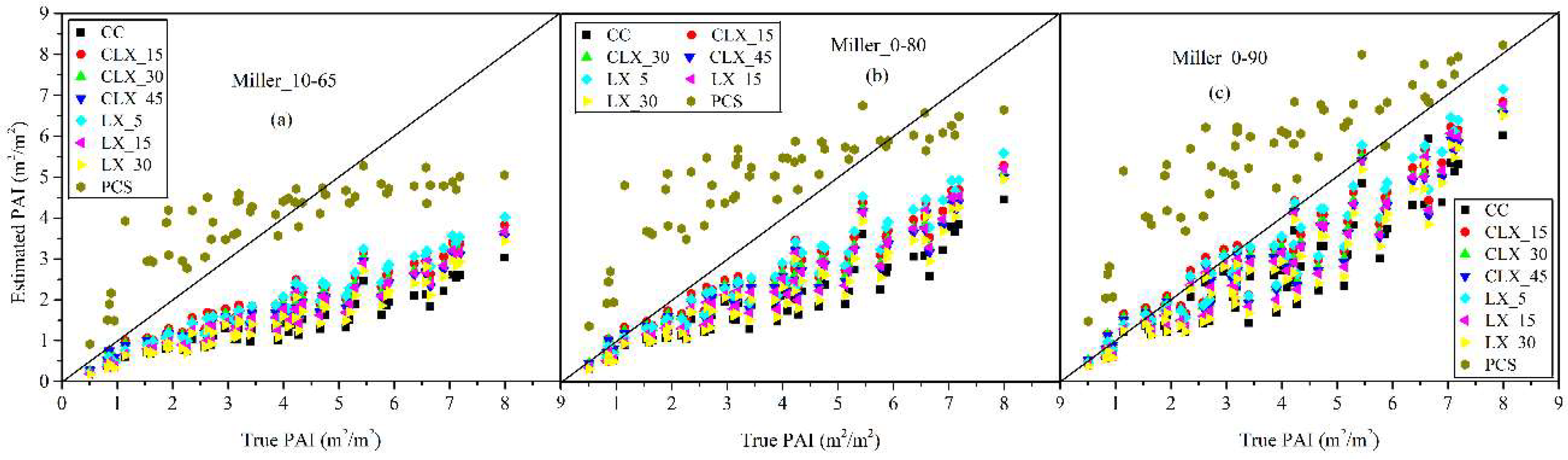
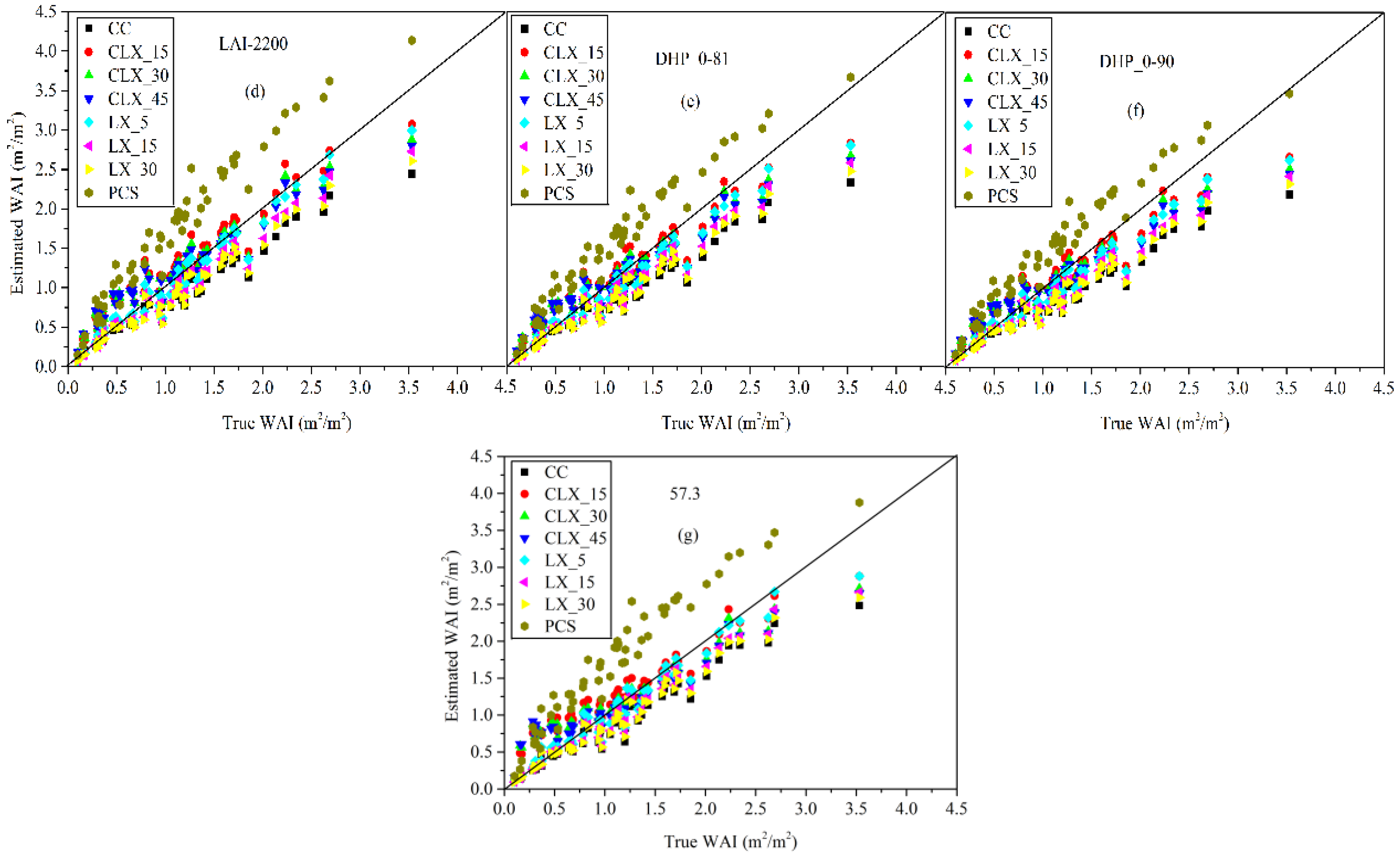
The distinct PAI underestimation for all the combinations of inversion model,
,
estimation algorithm, and segment size except those with PCS at the leaf-on deciduous scenes with PAI > ~3.5 (
Figure 9), indicating that the
of those scenes was not accurately estimated by the three algorithms of CC, LX, and CLX. Cutini et al. [
32] reported that the leaves of deciduous forest canopy tended to concentrate at the top crown to compete for light. Therefore, limited direct sunlight can penetrate through the top crown of these forest canopies and into the ground for those with large PAI. Furthermore, insufficient gap fraction or gap size measurements that the
estimation algorithms rely on to estimate
were collected from these leaf-on deciduous forest canopies would cause the
estimation algorithms to underestimate
. Thus, the
underestimation would be the main reason for the overall PAI underestimation at the leaf-on deciduous forest canopy with relatively large PAI. For leaf-on deciduous forest scenes, if the inversion models are the same, the combinations of inversion model,
,
estimation algorithm, and segment size with LX_5 performed the best, followed by the combinations with CLX_15 in the PAI estimation, except the combinations with Miller_10-65. This conclusion does not contradict the finding of Woodgate [
45] even though different tree species were examined in these two studies. Woodgate reported that CLX_15 performed the best compared with other combinations of
estimation algorithm (CC, LX, and CLX) and segment size (15°, 45°, and 90°) to estimate the
of eucalypt forest canopy, but LX_5 was not analyzed in that study [
45]. Better performance of LX to estimate the
of leaf-on
Gliricidia sepium forest canopy was also reported by van Gardingen et al. [
25]; they found that the PAI underestimation decreased from 50% to 15% after the PAI estimates were corrected by
derived using LX.
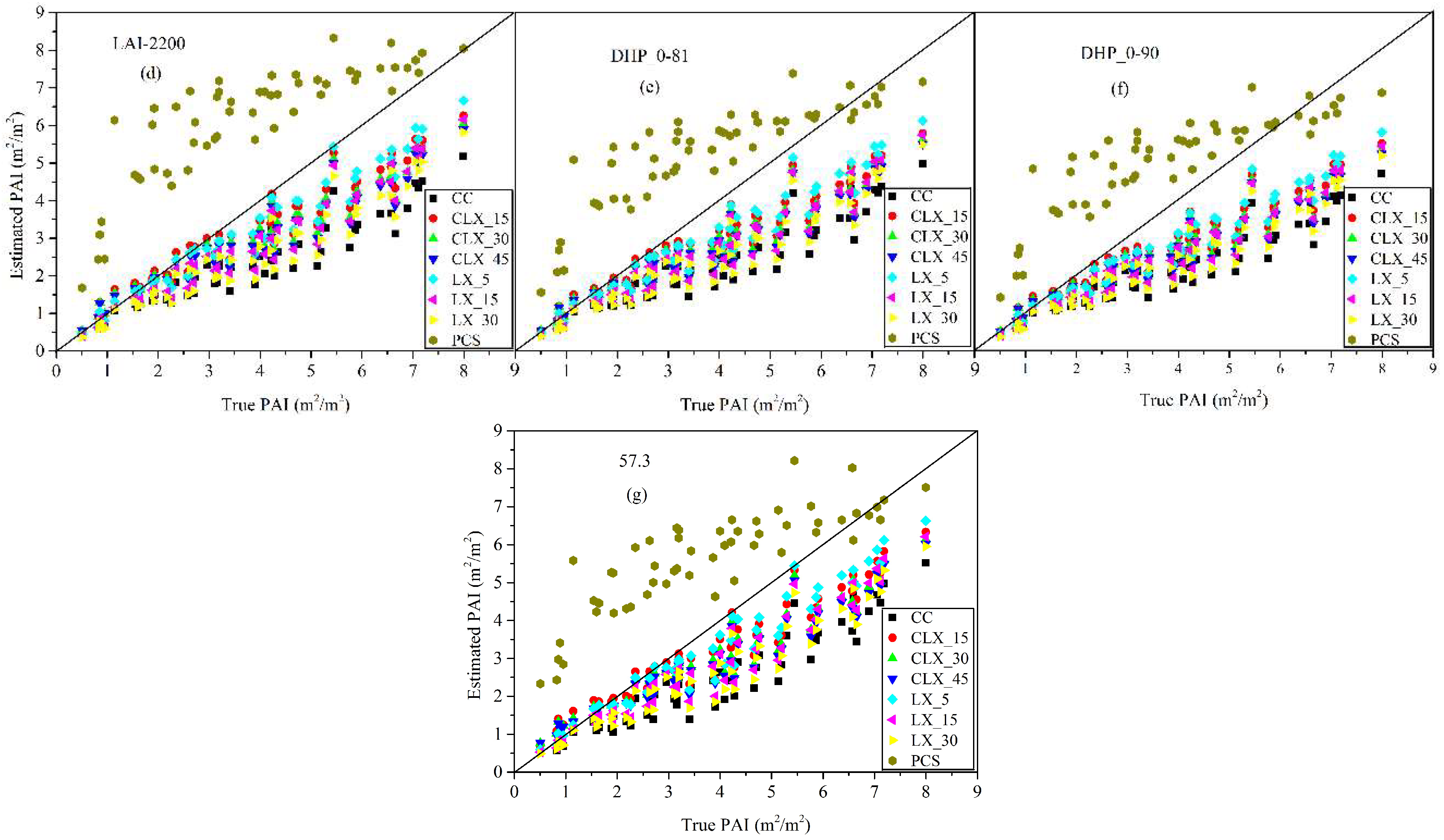
Compared with the leaf-on deciduous forest scenes, the gap fraction or gap size measurements collected at leaf-off deciduous forest scenes would be relatively sufficient as leaves were removed from the canopy and only woody components were left. Therefore, the accuracy of the
estimates estimated from CC, CLX, and LX at leaf-off deciduous forest scenes would be improved compared with those estimated at the leaf-on deciduous forest scenes. A sign of the improvement of the accuracy of the
estimates at the leaf-off deciduous forest scenes is that the WAI estimated from all combinations of inversion model,
estimation algorithm, and segment size at the leaf-off deciduous scenes were closer to the one-to-one line compared with the PAI estimated using the same combination of the inversion model,
,
estimation algorithm, and segment size at the leaf-on deciduous scenes (
Figure 9 and
Figure 11). The large slope and small RMSE and MAE of the combinations of inversion model,
estimation algorithm, and segment size with LX_5 except those combinations with Miller_10-65 and Miller_0-80 indicating that the
of leaf-off deciduous scenes can be accurately estimated if appropriate
estimation algorithm and segment size was adopted (
Table A2).
The PAI estimated from the seven inversion models except Miller_10-65 at the leaf-on coniferous forest canopy are close to the one-to-one line, except at the sub-series coniferous scenes of SPS (
Figure 8). This result indicates that the
of the sub-series coniferous scenes of JPSS and OPSW was accurately estimated by CLX if appropriate segment size was adopted. Furthermore, accurate PAI estimates can be obtained at the sub-series coniferous scenes of JPSS and OPSW if
and
were considered in the PAI estimation (
Figure 8 and
Table A1). For the sub-series coniferous scenes of SPS, the PAI estimated from all the combinations of inversion model,
,
estimation algorithm, and segment size at six scenes deviated largely from the one-to-one line, regardless of the inversion model,
estimation algorithm, and segment size used by the combinations, except those combinations with Miller_10-65 (
Figure 8). Upon further examination, the reference
of the six scenes range from 1.0 to 1.35. The stem distribution mode of five of the six scenes is regular. Currently, the
estimation algorithms except PCS used in this study cannot effectively deal with the situations of regular distribution of the canopy element in space at the scale of beyond-shoot. The
estimation algorithms would overestimate
in the six scenes with reference
≥ 1.0, as the
estimates obtained from these
estimation algorithms were always ≤ 1 (
Appendix C.3). Therefore, the
overestimation would be the reason for the severe PAI overestimation at the six scenes of the sub-series coniferous scenes of SPS. If the six scenes with reference
≥ 1 were removed from the sub-series coniferous scenes of SPS, then the combinations of inversion model,
,
estimation algorithm, and segment size with LX_15 would perform the best followed by combinations with the same inversion model but with CLX to estimate the PAI of the sub-series coniferous scenes of SPS, except combinations with Miller_10-65, Miller_0-80, and Miller_0-90. This finding is different from the conclusion of Pisek et al. [
60], who reported that CLX outperformed other
algorithms (CC, LX, and CMN) to estimate the
of an old Scots Pine plot with the age of 124 years. The one plot covered in the study of Pisek et al. [
60] and only six scenes of the sub-series coniferous scenes of SPS left after removing those SPS scenes with reference
≥ 1 may have contributed to the differences between the conclusions drawn from these two studies.
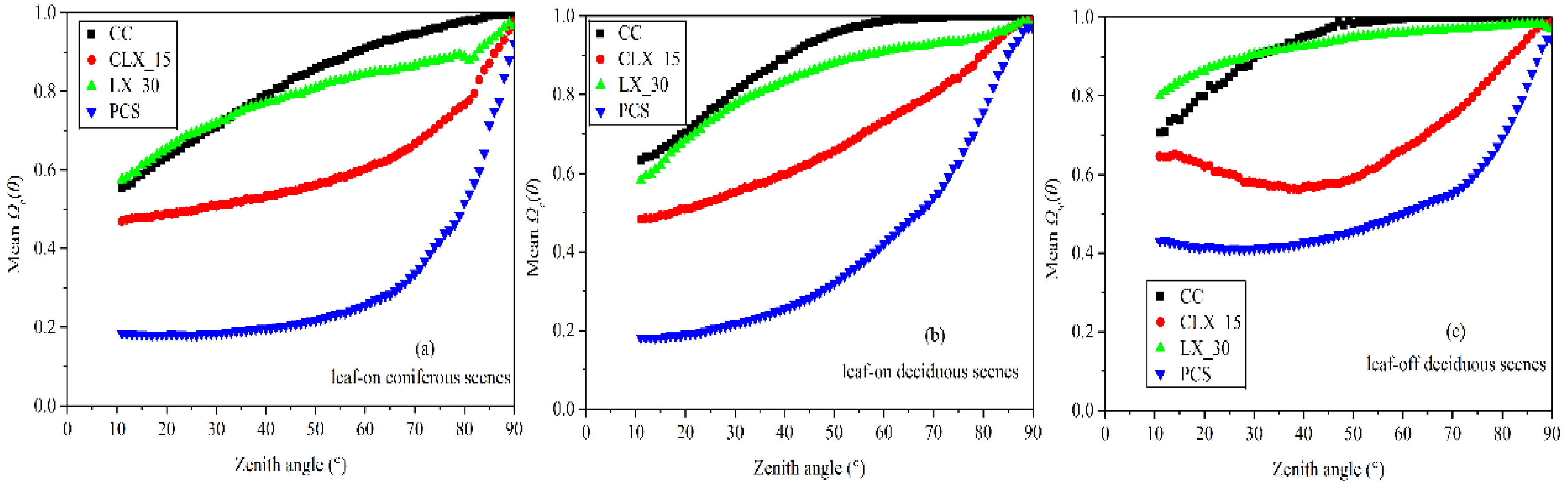
In conclusion, the best performance of
and
estimation algorithms in estimating the
and
of leaf-on and leaf-off forest canopy is the function of tree species and plant functional types. The different characteristics of the clumping effect of canopy element and woody component between the leaf-on deciduous scenes, leaf-on coniferous scenes, and leaf-off deciduous scenes and the obvious differences between the
and
estimates derived from the four
and
estimation algorithms (CC, CLX, LX, and PCS) with different theoretical basis have contributed to the different conclusions of the best combination of
and
estimation algorithm and segment size to estimate the
and
of the leaf-on and leaf-off scenes (
Figure 6,
Figure 8,
Figure 9 and
Figure 11,
Table A1 and
Table A2). No universally valid
and
estimation algorithm and segment size is available to accurately estimate the
and
of all leaf-on and leaf-off scenes, respectively. This finding indicates that there is still room to improve the performance of the currently available
and
estimation instruments and algorithms to accurately estimate the
and
of leaf-on and leaf-off forest canopy, especially for those canopies with reference
and
> 1 (
Appendix C.3).
There are several critical problems still existed for the four
and
estimation algorithms. For example, segment size is a key parameter for LX and CLX to estimate the
and
of leaf-on and leaf-off forest canopy. However, determining appropriate segment sizes of LX and CLX is difficult, particularly for the DHP approach [
18,
26,
45]. Gonsamo et al. [
26] reported that the
estimates derived from LX decreased evidently by decreasing segment sizes from 15° to 5° and slightly changed further by decreasing segment sizes from 5° to 2.5°. The minor variations in the
estimates obtained from LX using the latter range of segment sizes indicate that the spatial distribution of the canopy element in all segments was approaching the assumption of random distribution. Improved accuracy of
estimates obtained from LX with smaller segment sizes was reported by previous studies [
26,
45]. This trend was also observed in the present study (
Table A1 and
Table A2). However, the proportions of segments without gaps in all the segments also increased dramatically if small segment sizes were used to estimate
and
[
18,
26,
45]. The logarithm of the gap fraction of these segments without gaps gave undefined results, and a subjectively assumed PAI or WAI is typically assigned to these segments [
17,
26]. Therefore, the assumed PAI or WAI for the segments without gaps would be an error source for LX. On the other hand, the lack of ability of LX to recognize and utilize large gaps of between-crown clumping to estimate the
and
of leaf-on and leaf-off forest canopy remains unresolved, regardless of segment size ranging from large (120°) to small (5° or 2.5°).
Besides the two disadvantages of LX described, there are two more problems related to the small segment size faced for CLX. Firstly, the short length of segment increases the possibility of null gaps or full gaps in the transect of segment as reported previously [
18,
26,
45]. Secondly, the short length of segment will likely violate the assumption of an infinite horizontal plane defined by the CC algorithm [
58]. However, CC relies on the collected gap size measurements to evaluate the clumping effect of the canopy element and woody component at the segment scale. Therefore, the limited and insufficient gap sizes collected by CLX at the transect of each segment compared with TRAC would become the weakness of CLX in evaluating the clumping effect of the canopy element and woody component at the segment scale. The combinations of the inversion model,
,
and
estimation algorithm, and segment size with CLX did not always perform better than other combinations with the same inversion models but with different
and
estimation algorithms to estimate the PAI and WAI of leaf-on and leaf-off scenes (
Figure 8,
Figure 9 and
Figure 11,
Table A1 and
Table A2). This finding is not consistent with the conclusions of Gonsamo and Pellikka [
41], Leblanc and Fourier [
18], and Woodgate [
45] that CLX is better than other
estimation algorithms (CC, LX, and PCS) in estimating the
of the leaf-on forest canopy. Both the plant functional types, 3D forest scenes and segment sizes contributed to the differences between the conclusions drawn in the present and previous studies. The RMSE and MAE of the PAI and WAI estimated from the combination of inversion model,
,
and
estimation algorithm, and segment size with LX_5 at the leaf-on and leaf-off deciduous scenes were smaller than those estimated from the combinations with the same inversion model but with CLX (
Table A1), illustrating that the clumping effect of the canopy element and woody component at the segment scale was not thoroughly measured by CC for CLX.
For PCS, the significant PAI and WAI overestimation for the combination of the inversion model,
,
, and
algorithm and segment size with PCS illustrated that PCS overestimated the
and
remarkably at both the leaf-on and leaf-off scenes (
Figure 8,
Figure 9 and
Figure 11). The
and
overestimation for PCS was also reported in previous studies [
41,
43]. The combinations of the inversion model,
,
, and
estimation algorithm and segment size with CC underestimated the PAI and WAI of leaf-on and leaf-off forest scenes, except at the SPS coniferous scenes (
Figure 8,
Figure 9 and
Figure 11). This finding is consistent with the reports of Pisek et al. [
60], Leblanc and Fourier [
18], and Woodgate [
45] that parts of the large nonrandom gaps were not removed by CC, leading to an underestimation of
and
, and underestimated the PAI and WAI of forest canopy further.
Because the performance of the seven inversion models to estimate the PAI and WAI of the leaf-on and leaf-off forest canopy with consideration of
,
, and
were strongly dependent on the accuracies of the
and
estimates (
Table A1 and
Table A2) (
Appendix C.1). All the above-mentioned problems of the four
and
algorithms (CC, CLX, LX. and PCS) need to be solved reasonably in the future to improve the accuracies of the
and
estimates derived from the four algorithms.
5.4. Which Inversion Model(s) is (are) More Reliable to Estimate the PAI and WAI of the Leaf-on and Leaf-off Forest Canopy
The zenith angle ranges covered by the seven inversion models are apparently different. As explained previously, the zenith angle range covered by Miller_10-65 is the reason why the PAI and WAI estimated from the combination of the inversion model,
,
and
estimation algorithm, and segment size with Miller_10-65 were still smaller than those estimated from other combinations with different inversion models but with the same
and
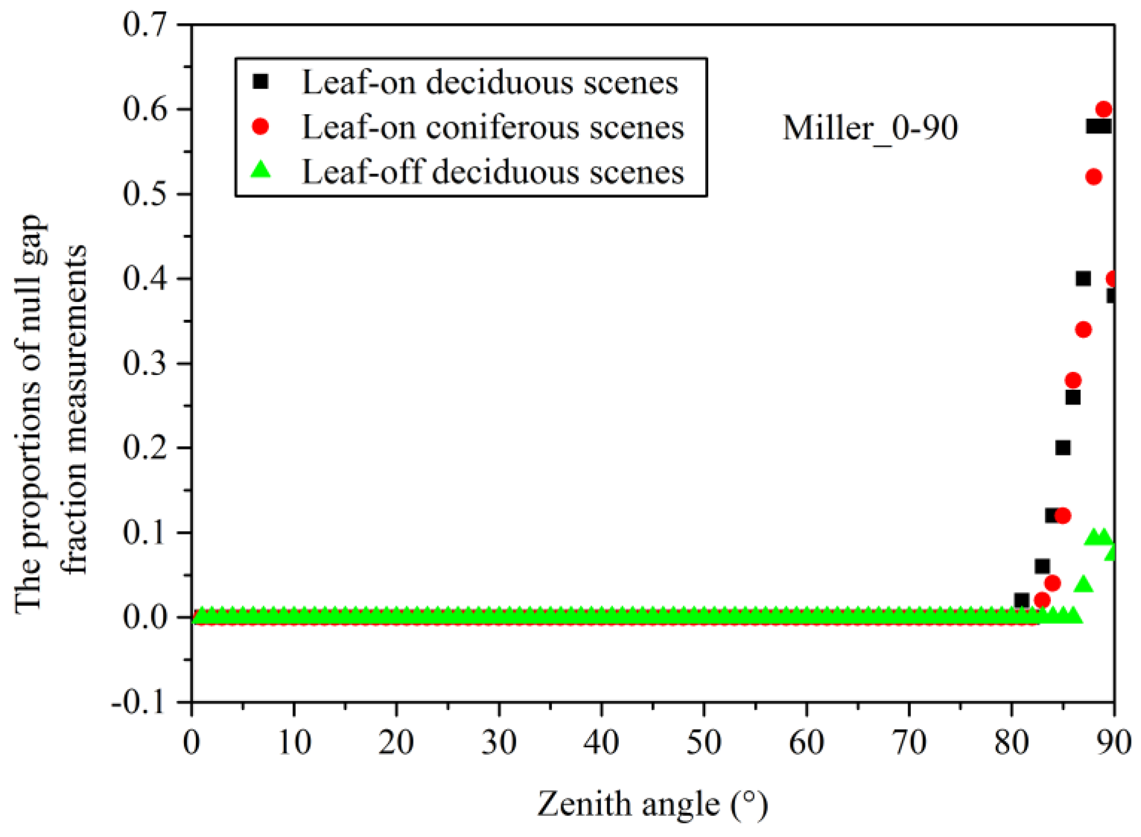
estimation algorithm and segment size. On the other hand, the PAI and WAI underestimation of Miller_10-65 illustrates the necessity of incorporating the gap fraction measurements at large zenith angles, which were not covered by Miller_10-65, to the PAI and WAI estimation of the leaf-on and leaf-off forest canopy. However, a problem in using the gap fraction measurements at large zenith angles in the PAI and WAI estimation is the high probability of obtaining null gap fraction measurements at these zenith angles, as reported by previous studies [
17,
25,
26] and the present study (
Figure 4). Several solutions were proposed to address the undefined inversion of the null gap fraction measurements, such as adding half or one pixel to the annulus of the DHP images or defining arbitrary upper PAI or LAI limit values of 8 or 10 [
17,
25,
26]. However, those proposed solutions cannot derive accurate PAI and LAI estimates for those annuli without gaps due to evident subjectivities. Therefore, the processing solutions of the null gap fraction measurements would produce estimation errors to the derived PAI and WAI estimates. Significant differences were observed between
and
or
and
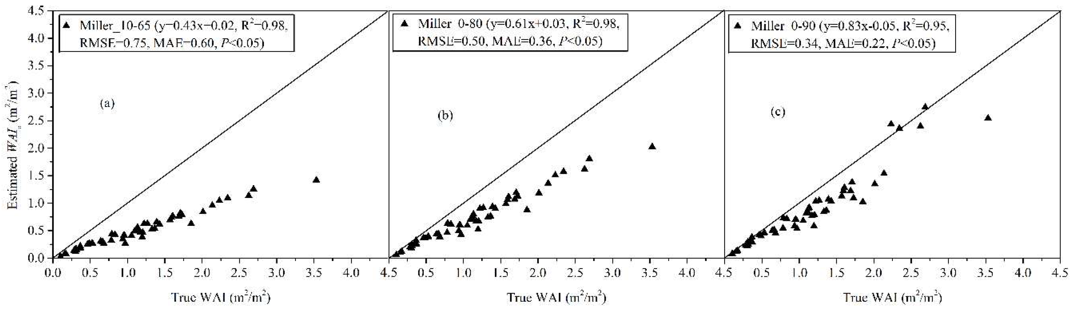
estimates at the leaf-on and leaf-off scenes, respectively, especially for those scenes with PAI~ > 2.5 at the leaf-on scenes and WAI~ > 2.25 at the leaf-off scenes (
Figure 7c,f and
Figure 10c,f) (
Appendix C.2). The significant differences indicate that the
and
estimation were largely affected by the processing solutions of the null gap fraction measurements as the null gap fraction measurements at the zenith angles close to the horizon were completely removed for DHP_0-90 at all annuli compared with Miller_0-90 (
Figure 4), and the same zenith angle range of 0–90° was covered by the two inversion models. Similarly, the PAI and WAI estimation errors of the processing solutions of the null gap fraction measurements can also be avoided for the two inversion models of LAI-2200 and DHP_0-81 as the same zenith angle width of annulus of 10° was adopted by the two inversion models to obtain the gap fraction measurements similar to DHP_0-90.
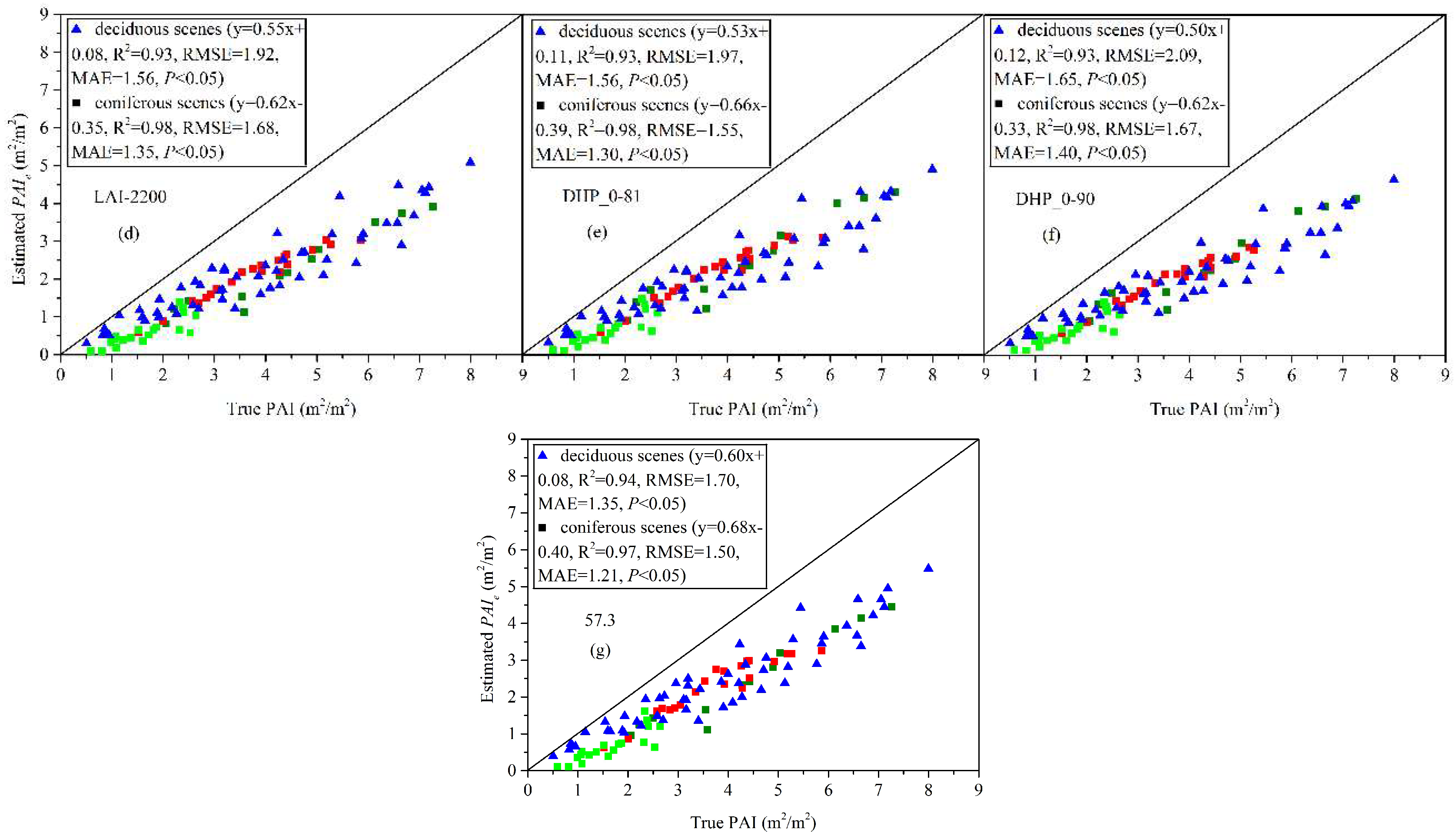
Compared with six other inversion models, the 57.3 inversion model shows three advantages in estimating the PAI and WAI of the leaf-on and leaf-off forest canopy. Firstly, the 57.3 inversion model is simple to apply. Furthermore, the
and
of leaf-on and leaf-off forest canopy can be assumed to be equal to approximately 0.5 at the zenith angle of 57.3°. Thus, no
and
measurements need to be collected in the field if the 57.3 inversion model would be used to estimate the PAI and WAI of forest canopy. Secondly, determining the exposure settings for imaging DHP photographs that can avoid overexposure near the zenith and underexposure near the horizon is difficult in the field. Accurate exposure settings to collect DHP images can be obtained due to the reason that only the gap fraction measurements with zenith angles near 57.3° are needed for the 57.3 inversion model. Thirdly, determining a reasonable threshold to binarize all the pixels of DHP images with zenith angles ranging from 0° to 90° is difficult because light conditions change across different image areas of the DHP images. Therefore, an accurate threshold that is used to binarize the DHP images can be obtained if only the pixels with zenith angles near 57.3° were considered for the PAI and WAI estimation. The 57.3 inversion model does not always outperform other inversion models to estimate the PAI and WAI of all leaf-on and leaf-off forest canopies although it can provide PAI and WAI estimates with relatively good accuracies compared with other inversion models if appropriate
and
estimation algorithms would be adopted, and the
,
, and
would be considered in the PAI and WAI estimation (
Figure 8,
Figure 9 and
Figure 11 and
Appendix C.1). With the merits of the 57.3 inversion model described, the 57.3 inversion model can be treated as an alternative choice to estimate the PAI and WAI of the leaf-on and leaf-off forest canopy if the best combination of inversion model,
,
and
estimation algorithm, and segment size remains unknown.
In conclusion, based on
Figure 8,
Figure 9 and
Figure 11,
Table A1 and
Table A2, we suggest that 57.3, LAI-2200, and Miller_0-90 followed by DHP_0-81, DHP_0-90, and Miller_0-80 to be used in estimating the PAI and WAI of the leaf-on and leaf-off forest canopy. The PAI and WAI estimated from Miller_0-90 were closer to the one-to-one line compared with those derived from DHP_0-90, although the impact of the null gap fraction measurements of each zenith angle on the PAI and WAI estimation was difficult to evaluate quantitatively in the field, caution is needed if Miller_90 would be used to estimate the PAI and WAI of the leaf-on and leaf-off forest canopy, especially for canopies with large PAI and WAI.
The performance of the seven inversion models to estimate the PAI and WAI of the leaf-on and leaf-off forest canopy with consideration of
,
, and
was significantly affected by the
and
estimation algorithm and segment size used, and also the true PAI and WAI, and the reference
and
of leaf-on and leaf-off forest scenes (
Appendix C). Therefore, the performance of the inversion model to estimate the PAI and WAI of the leaf-on and leaf-off forest canopy is the function of
and
estimation algorithm, segment size, reference
and
, PAI, WAI, and plant functional types. No universal best inversion model is available to estimate the PAI and WAI of all the leaf-on and leaf-off forest canopies even if
,
, and
were considered in the PAI and WAI estimation.


 ,
, 


