1. Introduction
Permafrost coasts make up to 34% of the world’s coastlines and retreat with an average rate of 0.5 m/yr [
1]. Dynamics of Arctic coasts composed of frozen unlithified sediments have a strong influence on terrestrial [
2,
3], marine [
4,
5], and atmospheric [
6] systems. In recent decades, coastal erosion accelerated in most of the polar regions due to rapid climate change, with its impact on the Arctic two times larger than on the rest of the world [
7,
8]. The decline of sea ice extent [
9,
10], storm frequency increase [
11,
12], thermal and wave action growth [
13], and sea-level rise [
14] have a dramatic impact on the arctic coastal dynamics [
15,
16,
17,
18,
19,
20].
Numerous studies provide detailed data on contemporary coastal dynamics at local [
21,
22,
23] and regional [
24,
25] scales. Studies on the Beaufort Sea coast [
26,
27] and the Chukchi Sea coast of Alaska [
28] showed an increase in retreat rates at the beginning of the 21st century. At the same time, little of the Arctic coast is covered by multi-temporal studies. Remoteness and vastness of the polar regions make it difficult to conduct comprehensive field studies on coastal erosion, and therefore, estimate reliable circum-Arctic trends. Application of remote sensing techniques, such as satellite and aerial imagery [
29,
30,
31], unmanned aerial vehicles (UAVs) [
32,
33,
34], light detection and ranging (LiDAR) [
35] surveys, etc., provides reliable data for observing, quantifying, modeling and monitoring coastal dynamics over vaster regions and larger time periods compared to instrumental measurements.
About 20% of the Kara Sea coasts are thermoerosional [
25] (
Figure 1). They retreat especially intensively due to their composition of ice-rich permafrost and the presence of ice wedges and massive ice bodies, their thawing is resulting in formation of retrogressive thaw slumps [
15,
36], thermoerosional niches and gullies [
37,
38]. Surveys of coastal dynamics in the Kara Sea region at Yugorsky Peninsula [
21,
39], Baydaratskaya Bay [
40,
41,
42], and Western Yamal [
25,
43,
44] revealed mean annual coastal erosion rates ranging from 0.5 to 2.5 m/yr, what is significant in comparison to other Arctic regions. Most of these works were based on the results of field monitoring along separate profiles, conducted for two or three decades. The profiles were typically set every 100–500 m. Such low spatial resolution made it challenging to estimate the relative input of different drivers into the resulting retreat rates. To reliably assess rates of coastal erosion and to determine the contribution of various factors, data with higher spatial and temporal resolution are required. Obtaining such data has become much easier in recent decades thanks to high-resolution aerospace imagery.
In the present study we consider the coast as the zone of modern wave action, including foreshores with beach ridges, beaches, coastal bluffs, and low-lying laidas (inundated during the highest tides and storm surges), as well as adjacent areas indirectly influenced by sea wave action (such as thermal gullying, khasyrei formation on the surface of terraces, etc.). We focused on coastline (top of the bluffs on the erosional coasts or dense vegetation boundary on the accumulation coasts) as indicator of shifting of the entire coastal zone.
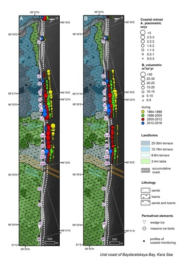
The present study aims at estimating rates of the coastal changes of Baydaratskaya Bay (Kara Sea) from the 1960s to 2016 using remote sensing accompanied by long-term field monitoring data. The Ural and the Yamal coasts of Baydaratskaya Bay were chosen as key sites because (1) they have different geomorphic and geographic conditions, which allows to estimate their impact on coastal erosion, and (2) the underwater part of the gas pipeline Bovanenkovo-Ukhta crossing Baydaratskaya Bay was built at these two sites in 2009–2012, making it possible to compare natural conditions with the period of human impact. For the first time, the rates of coastal retreat for these study areas were based on the interpretation of series of aerial and satellite imagery from the 1960s until 2016. Besides planimetric, we calculated volumetric rates of coastal retreat, which are more demonstrative, more relevant for coastal erosion modelling, and enable sediment flux calculation [
22]. An accuracy of calculated values was estimated. The spatial and temporal variability of retreat rates were analyzed. Analysis of spatial variations of permafrost conditions as well as temporal variations of climatic conditions allowed us to assess the possible human contribution to coastal dynamics.
2. Study Area
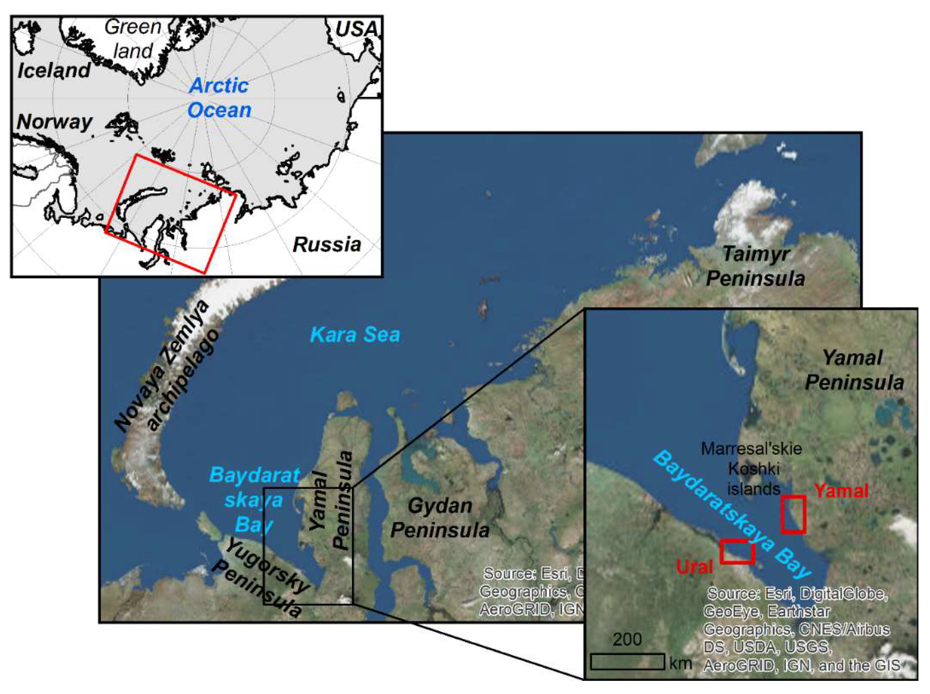
The Kara Sea is located in the western part of the Eurasian Arctic ocean shelf (
Figure 2). Two key sites of the study are located in the western part of the Kara Sea on the western (Ural) and the eastern (Yamal) coasts of Baydaratskaya Bay (
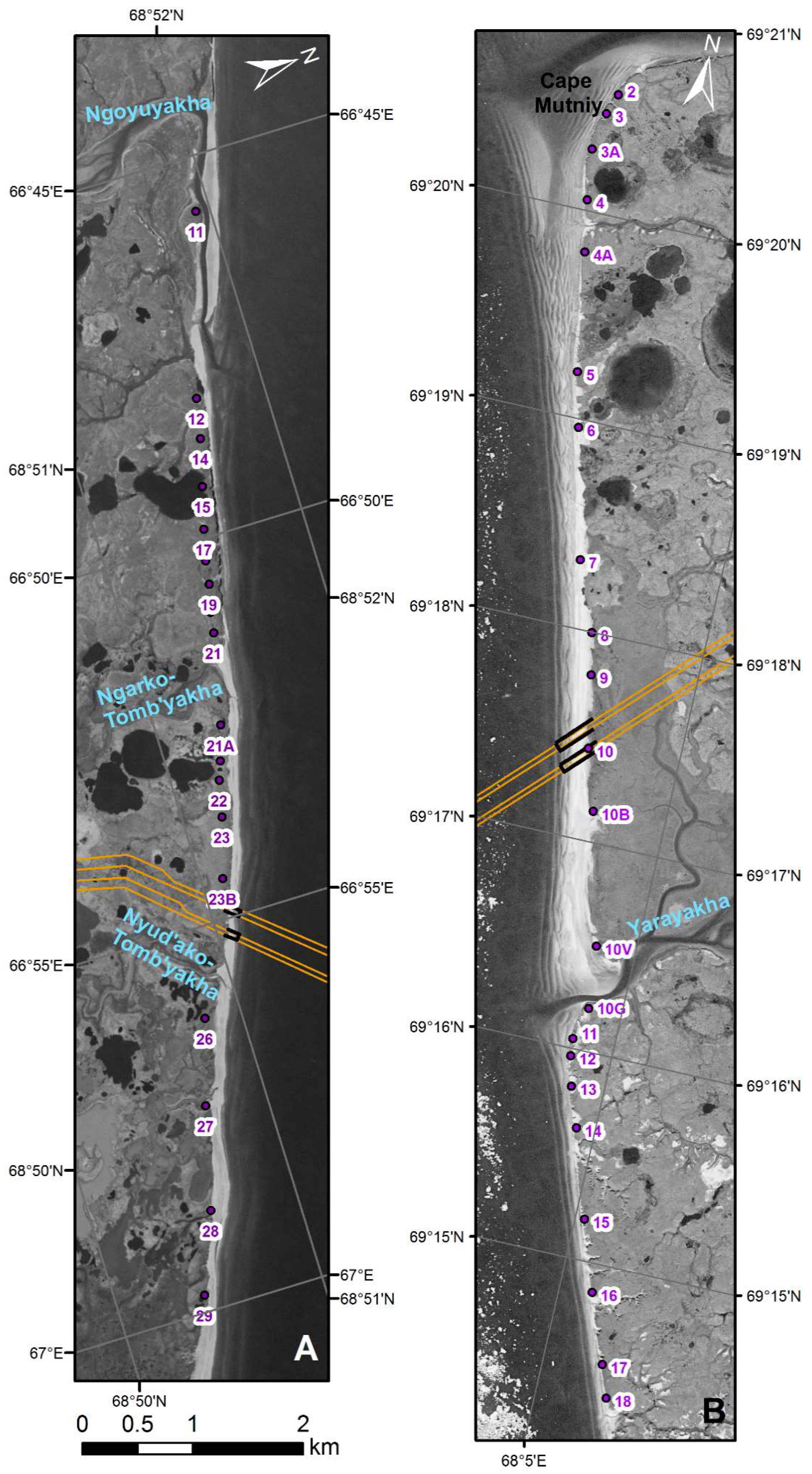
Figure 2). The Ural key area is an 11 km long coastal segment between the mouth of the Ngoyuyakha River in the west, and the laida (low surface inundated during the highest tides and storm surges) on the eastern side of the Nyudyako-Tambyaha River in the east (
Figure 3). The Yamal key area is a 12.5 km long coastal segment between Cape Mutniy in the north and the ravine 4 km north of the Liyaha River’s mouth in the south (
Figure 3).
The climate of the region is severe. Average annual air temperatures range from −7 to −10 °С [
45]. The cold period (the period with mean daily temperatures below zero) lasts for about 250 days, from October to the middle of June. The amount of annual precipitation is 300–500 mm. Strong winds and storms from the sea are frequent. In winter, the prevailing wind direction is seaward (from the south); in summer, it is directed inland (from the northwest). Inland-directed winds in summer provoke waves that transmit their energy to the coast and erode it during the ice-free period. In the warm period (June–September) the prevailing wind velocity is 3–6 m/s (50% of observations); in the cold period, it is 4–8 m/s (52%). The frequency of strong winds >10 m/s is 10% in summer and 20% in winter. The sea is completely ice-free for only two months (August–September). The maximum value of tide-driven (combined with wind-surges) sea level fluctuations is 0.8–1.0 m [
46].
The area is underlain by continuous permafrost, with thickness down to 40–50 m on the Ural coast and down to 50–100 m on the Yamal coast. The mean annual ground temperature at the depth of zero annual amplitudes ranges from −2 to −5 °C. The thickness of the seasonal thawing layer varies from 0.3–0.4 to 2 m [
46]. Thermodenudation processes, such as thermokarst, thermal erosion (gullying), frost cracking, and mass movements, are widespread.
The south-western Kara Sea shelf is shallow: its depths do not exceed 100 m. Depths of Baydaratskaya Bay are less than 40 m. The coasts are low swampy plains. Coastal plains at the Ural and Yamal key sites have several levels of topography, relatively similar to each other (
Table 1).
In 2009–2012, the underwater crossing of Baydaratskaya Bay by the gas pipeline Bovanenkovo-Ukhta was built. Two cofferdams, buildings, and roads were constructed at each key site; some dredging was done at the mouth of the Yarayakha River; sediments were excavated from the beach. Human impact also included heavy vehicles driving on the surfaces of low terraces, laidas, beaches, and tidal flats [
42].
3. Materials and Methods
3.1. Remote Sensing Data
The rates of coastal advance/retreat at Baydaratskaya Bay reach up to a few meters per year [
42]. Remote analysis of these dynamics demands high spatial resolution remote sensing data, its proper correction, and precise georeferencing. In this study, we used Corona KH-4, QuickBird-2, WorldView-2, and WorldView-3 optical space-borne and aerial imagery with spatial resolution from 7.5 to 0.3 m (
Table 2). We considered the dynamics of the two key sites of the Kara Sea for the whole period of study: 1964–2016 for the Ural site and 1968–2016 for the Yamal site, as well as for different periods: 1964–1988, 1988–2005, 2005–2012, and 2012–2016 for the Ural site and 1968–1988, 1988–2005 and 2005–2016 for the Yamal site, respectively (Figures in the
Section 4). During long-term time lapses (from the 1960s to 2005), we observed natural coasts that were undisturbed by human development, whereas the recent short-term time lapses (from 2005 to 2016) included the period of pipeline construction (2009–2013), which was supposed to influence the coastal dynamics.
To determine the position of the coastline in the 20th century, Corona satellite imagery and aerial imagery were used. Corona is declassified military satellite imagery from 1960–1972 with global coverage and the highest ground resolution of up to 1.8 m. It is distributed by the U.S. Geological Survey [
53] as scanned film strips 70 mm × 75.6 cm in size in four image tiles with a 7 μm (3600 dpi) scan resolution. Due to its large elongated coverage, Corona images are strongly affected by perspective distortions, especially on the margins [
30,
54]. Our study areas did not exceed 50 km
2 and are both located in the center of the film strips. Therefore, we did not undertake geometric correction of the whole strip. The part of the image covering key areas was referenced to the modern images with a spline transformation. Aerial imagery was acquired as analogue photographs with an 18×18 cm frame size and was scanned at a 40 μm (600 dpi) resolution.
For the 21st century (2005–2016), Digital Globe products (QuickBird and WorldView images) were used. They were provided as digital scenes with full metadata. Digital Globe products had the geolocation accuracy of 23 m CE90 for the QuickBird imagery and 5 m CE90 for the WorldView imagery.
The imagery we analyzed initially had the following levels of processing:
Raw images (Corona and aerial imagery): unprocessed. The metadata of Corona contained the entity ID (mission and frame numbers), acquisition date, camera type (aft/forward/cartographic/vertical), and camera resolution (stereo medium/stereo high/vertical low/vertical medium/vertical high). The metadata of aerial imagery implied flight and frame numbers, and acquisition date.
Standard (WV2 2016 for Ural, WV3 2016 for and QB2 2005 for Yamal): the imagery was radiometrically corrected, sensor corrected, and map projected, normalized for topographic relief with respect to the reference ellipsoid applying a coarse DEM.
Ortho Ready Standard (QB2 2005, WV1 2012 and WV2 2013 for Ural): the imagery was radiometrically corrected, sensor corrected, and map projected, had no topographic relief being applied with respect to the reference ellipsoid, making it suitable for orthorectification.
All chosen imageries were acquired from the end of May to mid-October when the water area was ice-free and the coastal bluff was not covered with snow.
Therefore, the imagery had a resolution appropriate to study coastal dynamics, but it required geometric correction (orthorectification) and thorough georeferencing before measuring coastal erosion/accretion rates.
3.2. Fieldwork
The Laboratory of Geoecology of the North, MSU, in cooperation with Zubov State Oceanographic Institute, carried out monitoring of coastal dynamics of the key areas since the 1980s. During numerous expeditions, recurrent (almost every summer) topographic surveys along a network of profiles (Figures 3 and 5) were conducted. The surveys started as direct measurements by tape; in the last decades, they were executed by a LEICA TCR802 or SOKKIA SET 230 RK3 total station. Last year, we combined tachymetric surveys around the gas pipelines with DGPS through a Javad Sigma G3T DGPS receiver both in RTK and in static modes along the profiles of the coastal monitoring network. The morphology, lithology, and permafrost of key areas as factors of coastal dynamics were mapped and described.
Application of the field data was restricted since it was collected during expeditions of the private company and the most of original data is not allowed for open publication. The present study was based on the remotely sensed data primarily. Among the field data, we used exclusively (1) DGPS GCPs for imagery referencing, (2) data on morphology, lithology, and permafrost conditions collected in field, and (3) mean rates calculated as a result of topography surveys along the profiles of monitoring to control our results.
3.3. Georeferencing and Orthorectification
The first step was referencing the 2016 WorldView images to a network of differential GPS (DGPS) ground control points (GCPs), which were collected during fieldwork in summer 2016, by a first-order polynomial (affine) transformation. The original geolocation accuracy of these images was claimed to be 5 m; as DGPS accuracy comprised a few cm, it was enhanced to 0.4–0.8 m. Creating a network of GCPs in tundra landscapes was challenging due to the paucity of well-identifiable stable features, such as man-made infrastructure in unsteady permafrost landscapes. Our DGPS GCPs network included buildings, cofferdams, pipelines, and roads in the center of the key sites. Earlier images were referenced to 2016 WV2 by a second-order polynomial with a large quantity of natural control points: small lakes, forelands of lakes’ shoreline, and corners of permafrost polygons. KH-4 Corona images were referenced by splines with as many control points as possible.
The studied territory is relatively flat with height differences of less than 30 m. Heights of coastal cliffs do not exceed 16 m at the Ural coast and 20 m at the Yamal coast. Through Equation (1), we calculated the uncertainty of relief-induced horizontal displacement (
δt) (in case of necessary data provided with the imagery):
where α is the tilt angle of the spacecraft and
h is the maximum relative height at the territory. The uncertainty varied from 3.2 to 6.6 m depending on the topography and tilt angle of the space imagery acquisition (
Table 2).
To reduce topography-induced distortions, we conducted orthorectification, where it was possible. We created orthomosaics from aerial photographs of 1988 using Agisoft PhotoScan Pro 1.4. We carried out orthorectification of the WV-2 2013 image of the Ural coast and the WV-2 2016 image of the Yamal coast applying freely distributed ArcticDEM ([
55], 5 m spatial resolution and 0.3 m vertical accuracy, according to [
56]) in ArcGIS 10.2 (ESRI). Possibly due to flat relief, the differences we revealed were negligible (up to 1 m) and appeared around the cliff bottom only, i.e., the position of the cliff top did not change after orthorectification. The offset between the standard product (orthorectified while using coarse DEM by the provider) and manually-rectified imagery was barely visible as well.
All the images were projected using the respective UTM zone (42N) on a WGS-84 datum.
3.4. Coastline Tracing and Quantitative Assessment of Coastal Dynamics
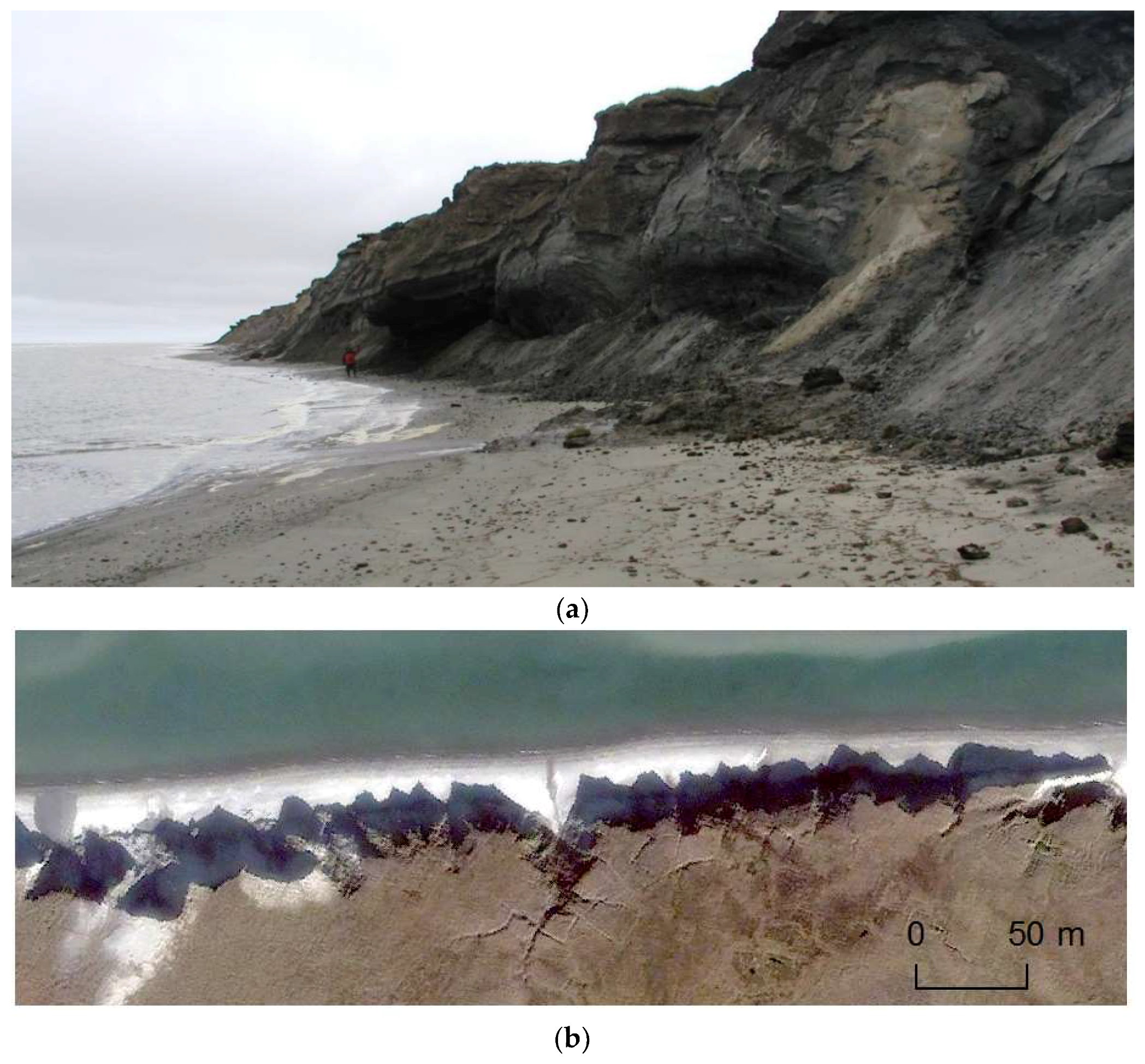
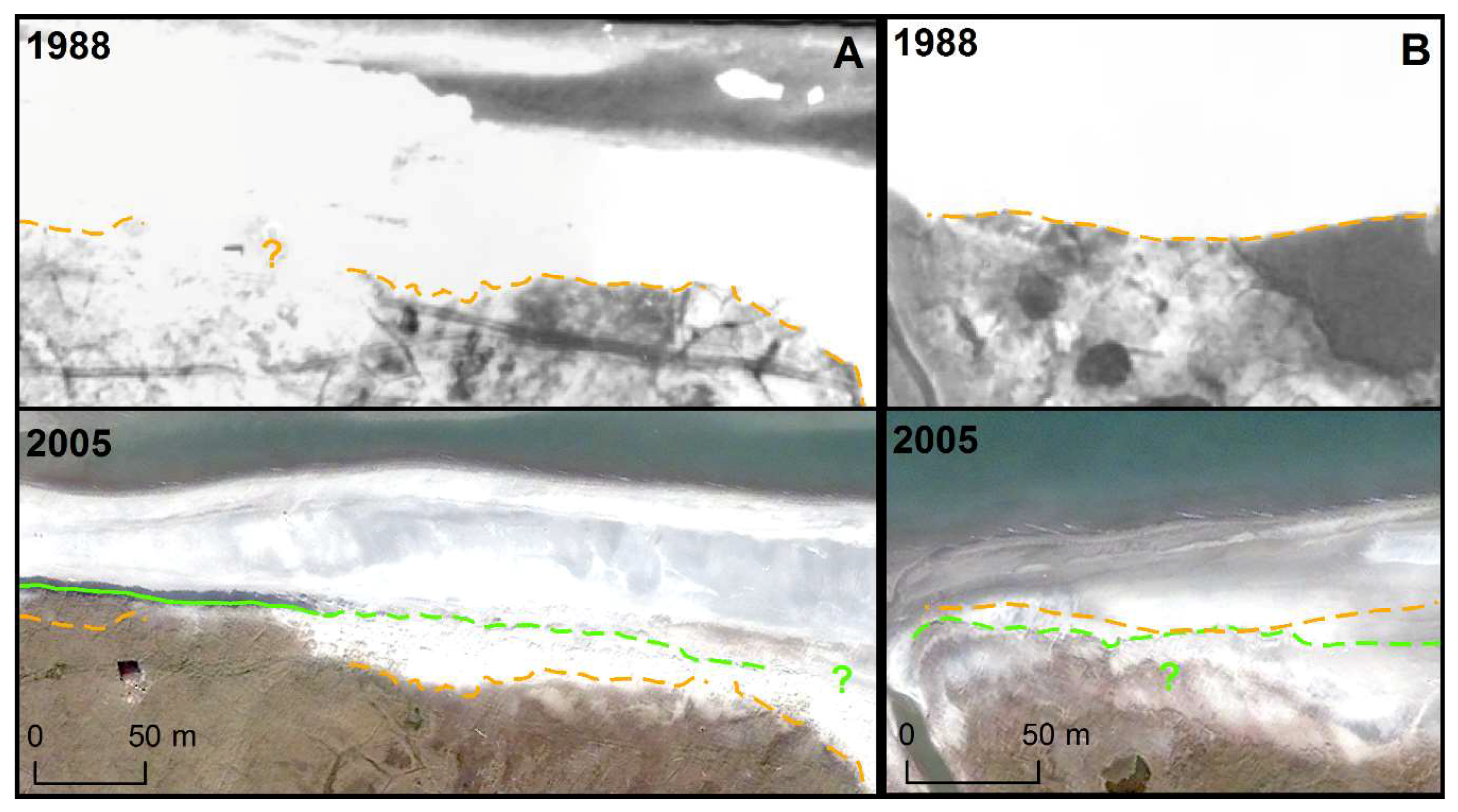
We traced the coastline along the top of the cliff at erosional sections and along the dense vegetation boundary (upper limit of high waves action) at accumulative sections. In some cases, tracing the coastline on aerospace images, and even in the field, was challenging and argued. For instance, in the study areas the cliff-top of the low-lying coastal plains was often buried by aeolian sands (
Figure 4A) or the dense vegetation boundary was unclear and gradual (
Figure 4B). Tracing the shoreline at such sectors was especially complicated, often impossible, on the bleached analogue aerial or Corona images of lower resolution. On the large sectors of pipeline and other infrastructure construction, the shoreline was substantially disturbed.
As the principal aim of the study was the analysis of coastal dynamics in permafrost conditions, we mainly focused on erosional segments composed of frozen deposits (while sandy spits, barrier beaches, and low-lying laidas of the accumulative segments are commonly unfrozen). Moreover, at the erosional segments the cliff-top as shoreline was definitely identifiable and had a clear unidirectional tendency to retreat, what made a detailed quantitative assessment of coastal dynamics possible here. Owing to foresaid, we accomplished quantitative transects analysis for these segments. However, adjacent accumulative segments were analyzed as well in order to obtain an integrative view of the process. For these segments, we provided a qualitative assessment with rates’ estimation for separate sections, where possible.
We digitized coastline manually using ArcGIS 10.2 (ESRI Inc., Redlands, CA, USA) software at pixel accuracy equivalent to scales from 1:300 to 1:2000. To calculate the shoreline position changes, we used the Digital Shoreline Analysis System (DSAS) of Thieler et al. [
57], available as an extension to ArcGIS. The program automatically creates transects normal to the general direction of the shorelines (baseline) with an optional spacing along the baseline. Then, it measures the coastal retreat rates as an offset from the baseline
L(ti) for imagery acquisition dates
ti, and calculates statistics on the overall retreat rates and their uncertainty. As coastal features and lithological units extended for hundreds of meters along the coast (see figures in the
Section 4), we considered 200 m as the lowest limit of spacing that provides consistent results. However, we arbitrarily assigned the spacing value to 50 m to ensure the visually continual set of transects for further analysis. We built transects for erosional segments of the coasts: 117 on the Ural and 128 on the Yamal. Transects crossing rivers and gullies, and areas of undefined coastline position were omitted from statistics calculation (20 on the Ural coast and 9 on the Yamal coast).
After digitalization, we calculated the retreat rates for each time span between imagery acquisitions in m/yr:
assuming
rL > 0 for progradation and
rL < 0 for retreat of the coast.
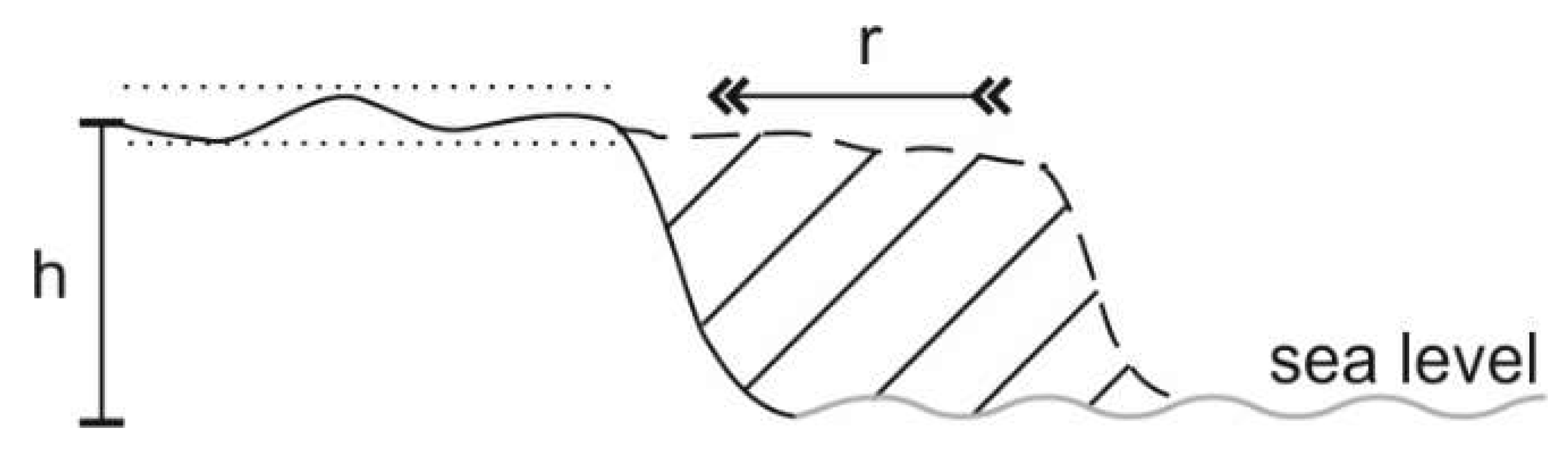
This parameter shows the velocity of the coastline movements in the plan (planimetric or linear), crucial for engineering. However, studies of sediment balance require knowledge of the amount of deposits that were eroded and accumulated. The volume of the eroded deposits can be assessed based on the obtained values of shoreline retreat (
rL) and the altitudes of transections extracted from ArcticDEM (
h) in cubic meters from one meter of shoreline (
Figure 5):
We classified coastline transects depending on their geomorphologic, lithologic, and permafrost conditions to reveal the impact of these conditions on spatial variations of coastal dynamics (
Table 1).
3.5. Uncertainty Assessment
The accuracy of the coastline position was estimated by adapting the method of Günther et al. [
30]. The following sources of uncertainties were taken into consideration:
spatial resolution of the imagery (δs);
relative georeferencing of two datasets to each other (δr); and,
topography-induced horizontal displacement (δot, δt, δat).
The first uncertainty δs is an arbitrary set value of how accurate the coastline could be digitized on a raster. For all of the remote sensing data it was assigned to be one half of the imagery spatial resolution as provided by an imagery distributor. Coasts where such accuracy was unfeasible were excluded from measurements. The uncertainty δr of the imagery georeferencing was obtained as the total RMS (root mean square) error in the link table, which was the geometric mean of mismatch of individual links to the referenced image.
The relief-induced error was calculated as:
where
α is the tilt angle of the spacecraft and Δ
z is the vertical accuracy of the DEM using for orthorectification. A straightforward method of estimating the vertical accuracy is to consider it equal to the variation of the sea surface height at the cliff bottom, which comprised Δ
z = 0.2 m. As a virtually flat surface of the sea was located just at the studied coastline, the accuracy of the DEM was clearly visible as both high-frequency noise and gradual offsets. However, for earlier imagery, no DEM was suitable, so we considered the eroded surface to be at the same height as the modern cliff, and derived the topographic-induced uncertainty
δt from the topography amplitude at the cliff (1) instead of the vertical accuracy.
Aerial imagery had overlapping coverage for the entire area, sufficient to build a three-dimensional (3D) model and an orthomosaic. As we had no reliable GCPs at that time, we built the orthomosaic in local coordinates with no prior parameters except the focal length
f = 200 mm and the frame size
s = 18 cm, and subsequently co-registrated the whole orthomosaic. The automatically-constructed model kept the sea surface flat and horizontal, so the main source of error was a high frequency noise, not exceeding
dz = 2 m, which might cause a horizontal offset of not more than:
The oldest available imagery for the study area was KH-4A Corona scanned films. As no acquisition geometry was known and the films were occasionally distorted [
30,
54], we preferred to co-register the raster using a spline function with tie points only in the neighborhood of the study areas. Here, the best estimation of accuracy was the RMSE of the control points offset at the co-registration.
All of the mentioned error sources resulted in an overall error as independent sources:
for orthorectified imagery,
for non-rectified imagery,
for aerial imagery,
for KH-4 Corona.
The total uncertainty of the rate of the changing coastline position from
x1 to
x2 during the period from
t1 to
t2 was calculated as:
The volumetric approach uses heights of eroded surface as well as rates of planar retreat, so the total uncertainty of volumetric rates
δrV comprised:
where
δh is an accuracy of estimation of the eroded surface height, depending on the surface roughness and equal to the height variance of the eroded surface at the current cliff.
3.6. Hydrometeorological Stress Calculation
The temporal variability of erosion rates in natural conditions in permafrost areas depends on a combination of two main factors, enhancing each other: the thermal and the wind-wave energy conditions. The thermal factor is determined by positive air temperatures, providing the thawing of permafrost in coastal bluffs. The wind-wave energy depends on the ice-free period duration, length of the wave fetch, sea depth, and wind velocity [
42]. It controls how fast the thawed material is removed by waves; calculating its changes is therefore, important for the understanding of coastal retreat mechanisms in the Arctic regions [
11,
24,
26,
58]. With ongoing climate warming, both air temperature and wind-wave energy increase; however, their changes are not simultaneous and they do not always directly relate to coastal erosion rates [
25].
The thermal potential of thermodenudation was estimated by the air thawing index showing the number of positive Celsius degree-days per year. A similar parameter called degree days thawing was used in [
58]. The ERA-Interim [
59] reanalysis was used. Previous studies showed [
13] that the reanalysis-derived absolute values could not be used without validation to observation data and removing the systematic error, which might reach 12–20% of the mean value. As far as there are no regular observations at the Yamal and Ural coasts, we used the anomalies (deviations from the long-term 1979–2017 mean) and did not appeal to absolute values.
To calculate the wind-wave energy flux, we applied the Popov-Sovershaev method, which is based on the dependence of the energy flux on ice-free period duration, wave fetch along the wave-dangerous wind direction, wave-dangerous wind direction frequency, and wind speed in third degree [
42]. For wind characteristics, we used ERA-Interim data [
59]. The ice-free period duration was estimated using OSI SAF daily sea ice concentration data in 12.5 km resolution net of © (2018) EUMETSAT [
60]. Wave fetch and wave-dangerous wind directions were derived from ETOPO-1 digital elevation model [
61].
The total hydrometeorological influence on coastal dynamics was roughly bounded by a sum of air thawing index and wave energy flux anomalies normalized by standard deviation [
13].
5. Discussion
5.1. Application of Remote Sensing for Studies of Coastal Dynamics in the Kara Sea Region
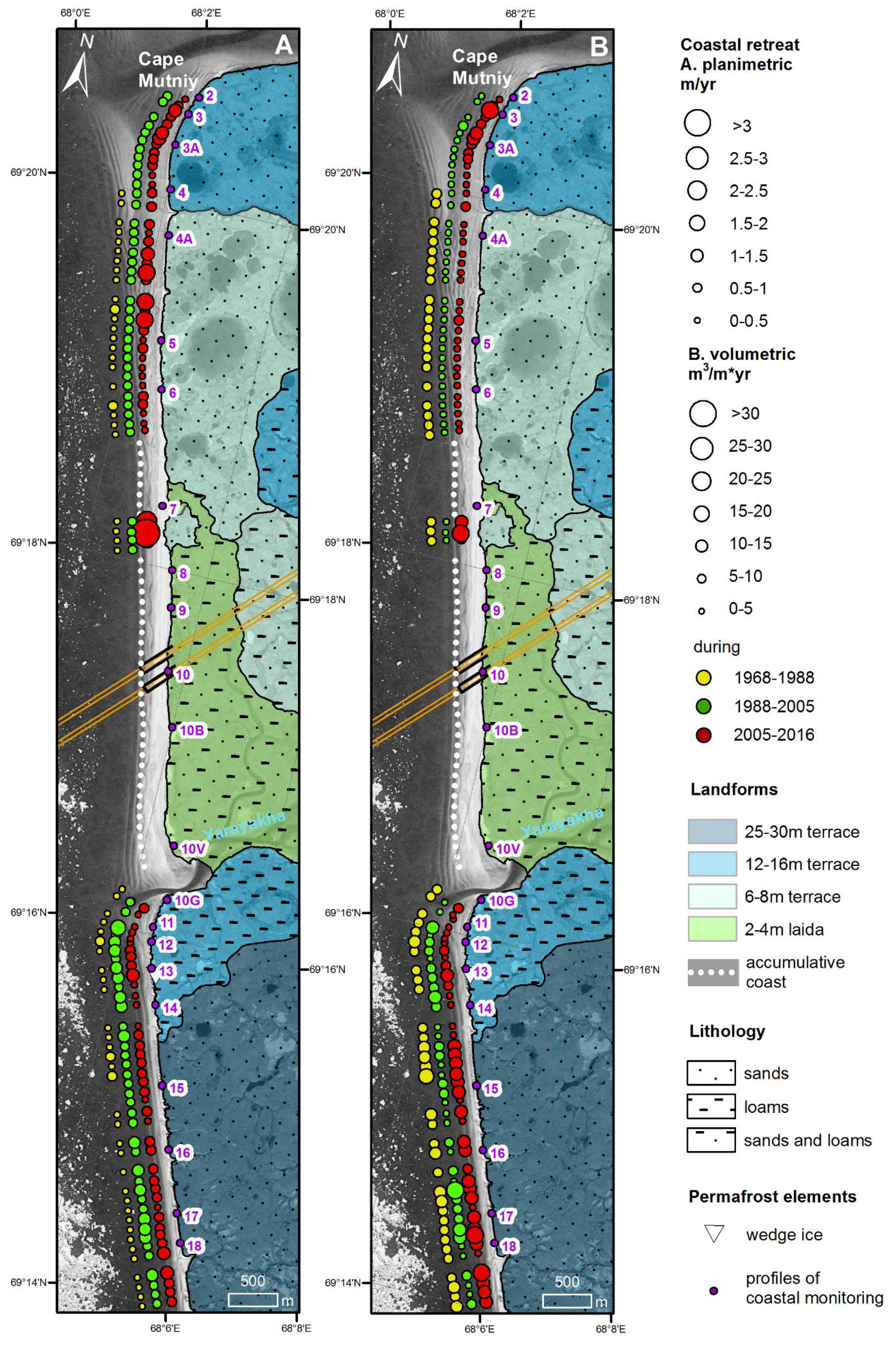
Remote sensing has shown its good applicability for studies of coastal erosion in permafrost areas of Western Siberia. It provides detailed, reliable, and comprehensive information on coastal dynamics. The great advantage of aerial and space imagery application is their easy accessibility due to relatively low price and large coverage. In remote areas with high transportation expenses, such as the Kara Sea region, remote sensing data may replace, or considerably complement, fieldwork. Moreover, if field monitoring on the coasts of Baydaratskaya Bay was launched in the 1980s, the first satellite imagery for this region was acquired in the 1960s, which allows to extend the period of studies. Another advantage of remote sensing is the possibility to obtain a spatially continuous record of coastal retreat, contrarily to surveys along profiles, where sections with the highest retreat rates may be situated between profiles, and thus, remain unobserved. For instance, at the Yamal coast, the greatest erosion rates fall into the area south of profile 7 (
Figure 6A), uncovered by field measurements. Using DEMs allows relatively precise estimation of volumes of eroded material, which is especially important in the application of studies of sediment fluxes, carbon fluxes, etc. [
30,
62].
However, working with remote sensing data for coastal dynamics studies, we faced some issues. Firstly, the accuracy of the obtained data was relatively low and required improvement: 0.15–0.45 m/yr for planimetric rates while the values of these rates were 0.1–5 m/yr, and 1.1–10 m3/m/yr for volumetric rates while the values of these rates were 0.5–20 m3/m/yr. The uncertainties could be decreased by obtaining imagery with higher spatial resolution, more thorough georeferencing, and orthocorrection of the imagery using stereopairs. Nevertheless, the erosion rates calculated using remote sensing methods showed good agreement with field monitoring data. Coastal retreat rates that were obtained by direct measurements from stable benchmarks for separate profiles had higher accuracy than the rates calculated from aerial and satellite imagery (up to 0.1 m/yr). The average retreat rates for the Ural coast from 1988 to 2016 were estimated as 1.4 ± 0.15 m/yr by aerospace imagery, as compared to 1.6 ± 0.1 m/yr according to observational data. For the Yamal coast, the 1988–2016 average rates obtained by remote sensing data analysis were 0.4 ± 0.16 m/yr, compared to 0.6 ± 0.1 m/yr according to field surveys. Therefore, remote sensing data provided relatively accurate results in assessing long-term erosion rates at large sections.
Additionally, it may be complicated to provide necessary temporal coverage by images due to their low frequency of acquisition or their high cost. It is especially significant while studying the dynamics of accumulative coasts, which are often more changeable and have no direct trend of migration. New remote sensing techniques, such as LiDAR and structure from motion by UAV images, provide more precise and recurrent data [
33,
35]. Although estimating temporal variability of coastal dynamics using aerospace imagery is limited, they allow drawing general conclusions about changes in retreat rates over time.
5.2. Drivers of Coastal Dynamics
Based on aerial and satellite imagery interpretation and field data with regard to the previously published studies, we propose the following main drivers of coastal dynamics in the study region and investigate their spatial and temporal variability. Temporal variability of coastal dynamics was determined chiefly by the weather conditions, which were hard to detect with the help of remote sensing. In this regard, in the paper, we focus mainly on the factors of spatial variability of coastal dynamics.
5.2.1. Spatial Variability of Coastal Dynamics
Exposure of the Coasts
Exposure of the coast to the waves from the open sea generally determines regional-scale variability of coastal retreat, as coastlines in permafrost areas are usually relatively straight, and their exposure does not vary significantly at a given site. The location of two coasts of Baydaratskaya Bay in relation to other shores and islands is presumably the main factor in determining the difference in their average long-term retreat rates. Coasts of the Ural site are eroded four times faster than coasts at Yamal because of their exposure to the NNE winds and strong waves from the open sea. The Yamal coasts, on the contrary, face to the southwest, with a relatively small wave fetch. They are protected from high waves by the Marresal’skie Koshki Islands. The exposure of the coastal segment, therefore, influences the whole key area, not separate landforms or profiles. It also plays an especially important role, because the climatic and geologic conditions on both coasts are relatively similar. Local-scale spatial variability within the key sites is governed by other factors.
Sediment Balance and Longshore Sediment Fluxes
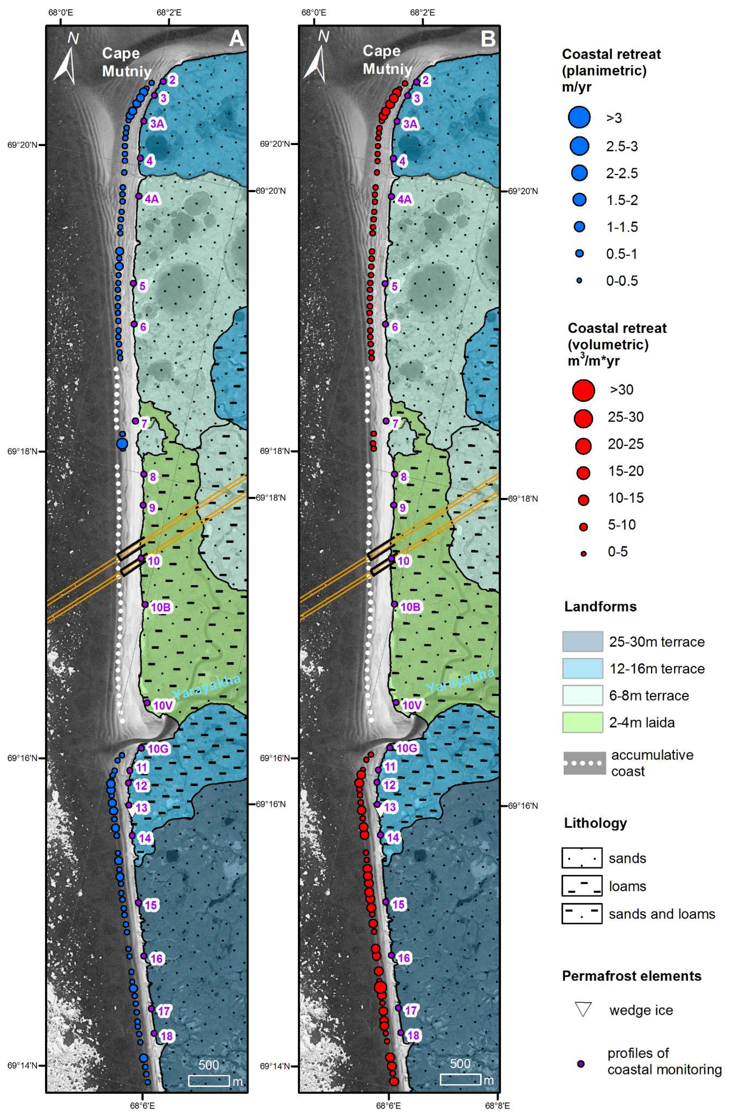
On the Yamal coast, the zone of divergence of longshore wave energy fluxes determines the area with the greatest average multiannual retreat rates to the south of the Yarayakha river mouth near profiles 17 and 18 (
Figure 9). The main longshore flux starting from here is directed towards the north, to Cape Mutniy; the second one comes to the south. As a result, this coastal segment experiences high planimetric retreat (0.6 m/yr) and the greatest volumetric erosion (10 m
3/m/yr).
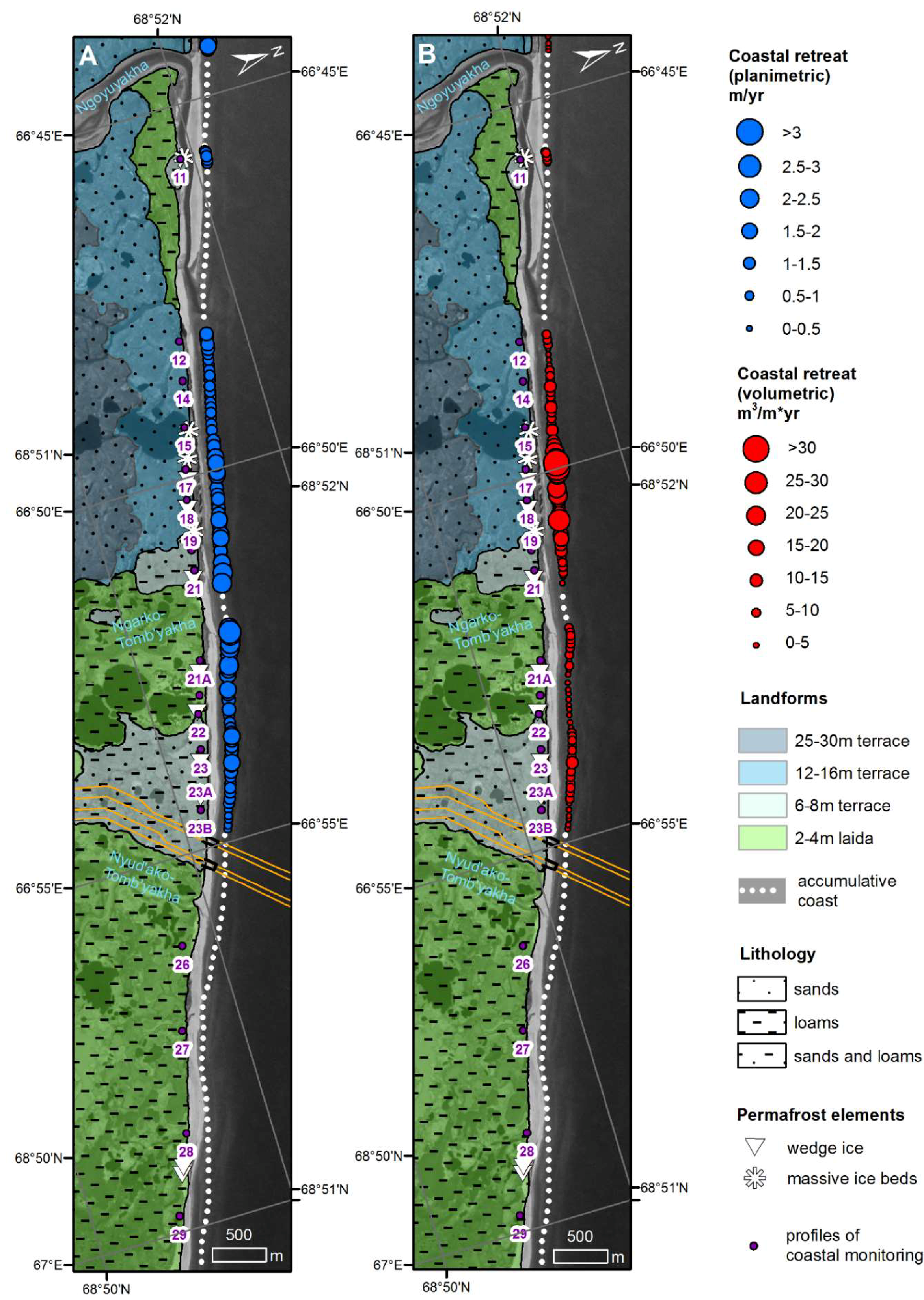
On the Ural coast, the longshore wave energy flux is directed to the south-east along the coast. Due to this, in undisturbed conditions prior to the pipeline construction (in 1964–1988 and in 1988–2005), on the sector of profiles 12–22 (
Figure 7), the sediment flux was deficient [
46] and coastal erosion prevailed. To the southeast (profiles 26–29), the flux was overloaded and sediments accumulated. After the construction, the westerly (entering) angle of the cofferdams served as a sediment trap; consequently, laidas near profiles 26–29 retreated at catastrophic rates between 2005 and 2012 (
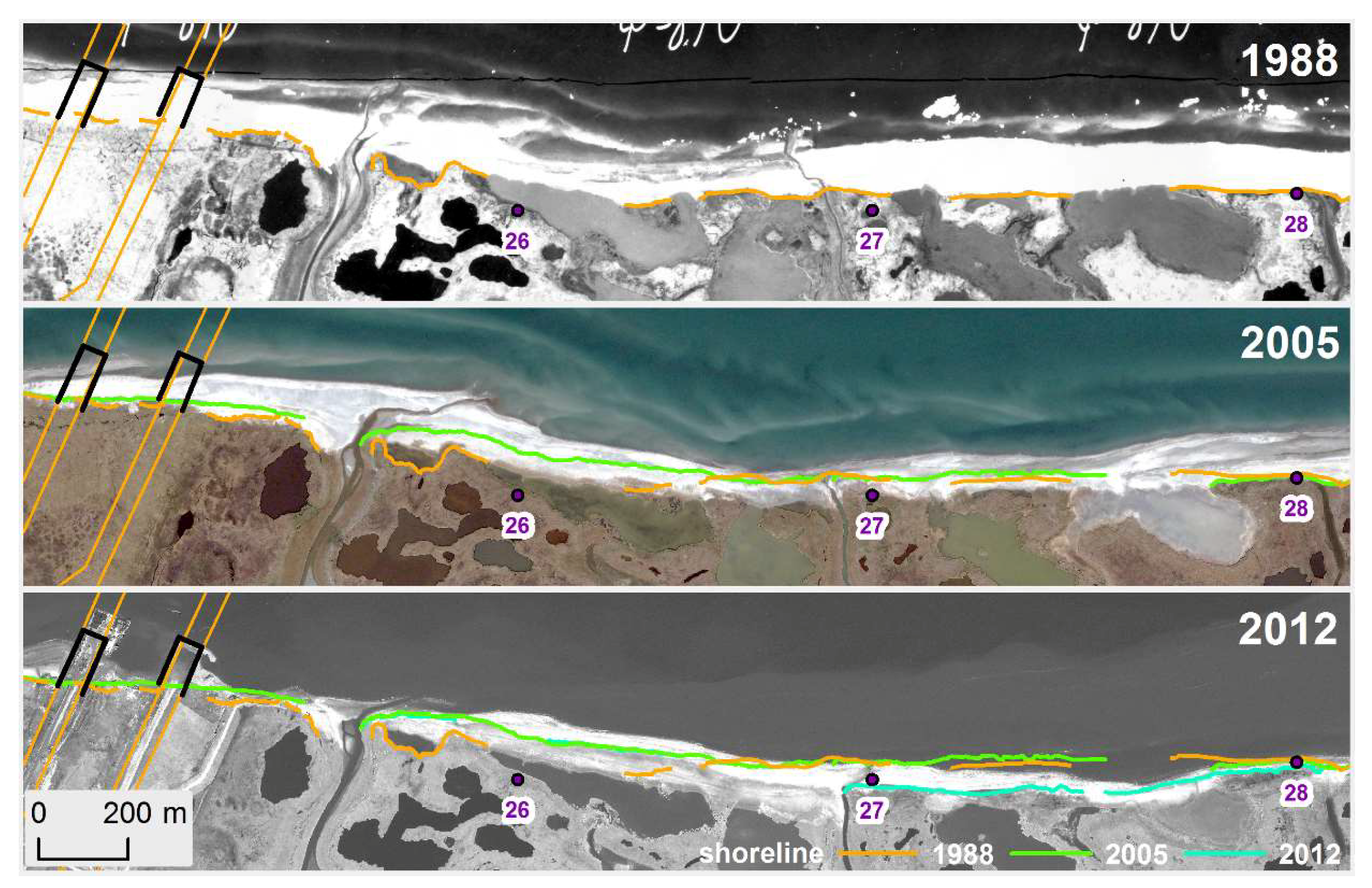
Figure 7). The beach to the east of the cofferdams also retreated by 80 m in 2005–2012 (
Figure 8).
An example of natural processes that are connected with sediment redistribution in the coastal zone is the segment near profile 11 on the Ural coast, on an isolated remnant of the 6–8-m terrace (
Figure 7). In 1964, a spit formed at the mouth of the Ngoyuyakha River. Then, in 1988, the channel dividing the spit from the bluff became inactive, and the spit served as coastal protection. As a result, in 1964–2005, the coast experienced very little retreat. In 2005, the old spit started to erode by longshore wave energy fluxes, and a new spit started to grow at the Ngoyuyakha River mouth. As the spit no longer protected the coast, erosion experienced acceleration, which started in 2005–2012 and continued in 2012–2016. From 2012 to 2016, the retreat rates rose by seven times, as compared to 1964–1988 (about 20 m
3/m/yr compared to about 3 m
3/m/yr, accordingly,
Figure 7). Such fast erosion was caused by natural cyclic processes of sediment redistribution in spite of a wind-wave energy decrease in 2012–2016, while the rest of the coastline became relatively stable.
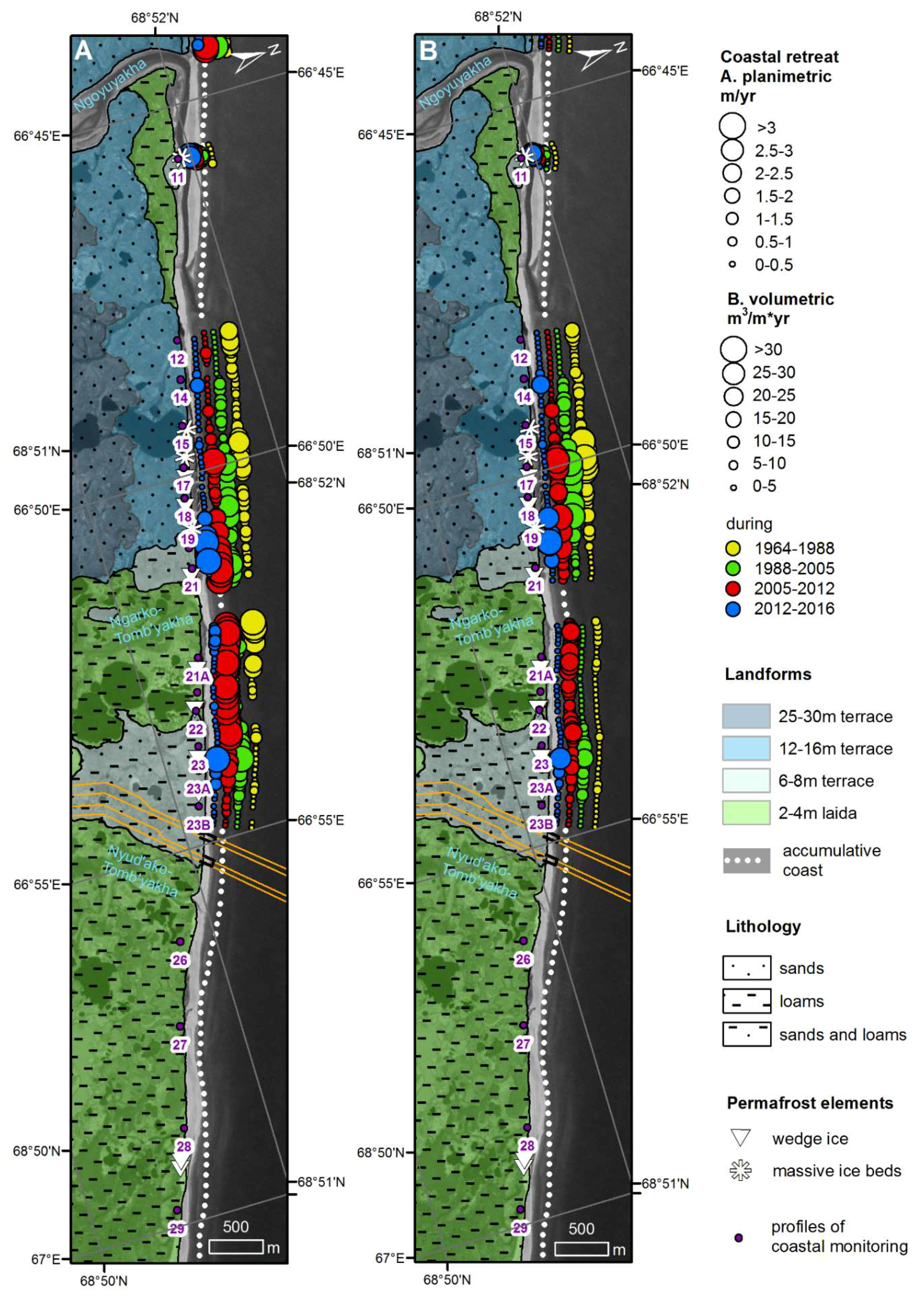
Generally, data on the Ural coast showed a shift of the greatest erosion rates from the west to the east (starting at profiles 15–17 in 1964–1988 and moving towards profiles 19–21 in 2012–2016). Such behavior might be caused by changes of the longshore sediment fluxes as a result of a change in the sedimentation regime after the shift of the mouth of the Ngoyuyakha River to the west. A similar situation was described near Kharasavey settlement, Western Yamal [
19], where a shift of the zone of divergence of longshore wave energy fluxes determined the shift of maximal retreat rates’ spatial distribution.
Morphology of the Coasts
The height and morphology of the coastal bluffs is essential in speaking of planimetric retreat spatial distribution. A storm that causes slight retreat of high cliff (with large volumes to erode) can provoke sudden and dramatic changes on low coasts. Little material needs to be washed off for their catastrophic linear retreat. Therefore, theoretically low coasts are more vulnerable to erosion rather than high coasts, however in fact it does not work always [
1,
63]. According to previous estimations [
64], laidas of the Ural coasts were considered one of the most stable segments in the area: 0.4–0.6 m/yr retreat from 1988–2006. However, according to our results, from 2005–2012, their erosion accelerated greatly, resulting at almost 10.0 m/yr linear retreat at some locations, with average rates for laidas reaching 7.0 m/yr.
The morphology and width of beaches and tidal flats, which are difficult to assess on satellite imagery because of the varying sea level (the tidal range is 0.8–1.1 m, the surge height is up to 1.5 m [
46]), also play an important role in spatial variability of coastal bluffs’ retreat [
63]. Beaches and tidal flats protect the cliffs from destruction [
65]; their width and inclination are one of the main coastal stability parameters [
66]. The greatest deformations of marine accumulative surfaces estimated for the Kara Sea region (Marresale) reached 0.3 m down in 2010 [
43]. On the Ural coast of Baydaratskaya Bay, the width of beaches significantly grew in 2005–2016 near the bluffs of the 12–16-m terrace (profiles 15–17,
Figure 7). As a result, these coasts were relatively stable from 2012–2016, when compared to the adjacent segments near profiles 19–21.
Lithology and Ground Ice
The general pattern of erosion rates’ distribution showed that they were relatively uniform at the Yamal coasts, with few spatial changes, while at the Ural coasts, the retreat rates varied greatly from segment to segment, and the position of the fastest retreating segments changed through time. We suppose that the main factors causing such difference are sediment composition and ground ice content in the bluffs. All levels of coastal plains at Yamal were predominantly composed by sand; no significant outcrops of large massive ice beds were found [
51]. On the contrary, cliffs of the Ural coast had a heterogeneous lithological composition: sands, silts, clays, and peat outcrop at different segments. Large massive ice beds of up to 80 m in length and 4 m in thickness were found at higher bluffs [
51], while cliffs that were lowered by thermokarst contained wedge ice networks. This created great spatial variability between small segments. Dallimore et al. [
67] showed that the presence of different types of ground ice facilitates coastal erosion. With growth of ground ice content capacity of the coasts for erosion rises, at least on the local settings [
68,
69]. High ice content creates favorable conditions for extremely fast retreat [
37,
38], especially under the conditions of climate warming [
26]. Increased erosion rates in areas of high ice content in sediments were also noted for the Marresale area, Kara Sea: an ice content increase from 10% to 60% provokes the growth of erosion rates by 1.5–2 times [
70,
71]. In the eastern part of the Arctic, on the Laptev Sea coasts, the average retreat rates for the Ice Complex segments are 1.9 m/yr, when compared to 0.3 m/yr for areas without the Ice Complex [
72].
However, although both sediment composition and ice content influence retreat rates, they are not directly connected. The presence of ground ice, on the one hand, leads to a faster thawing of the bluff. On the other hand, when frozen, the icy cliff can be resistant to waves, similarly to lithified rocks. The amount of heat required for thawing of the ice increases as well, slowing down the erosion. However, excessive ice content leads to a deficiency of sediment flux to the coastal zone and consecutive erosion enhancement [
3,
66]. The influence of sediment composition on coastal retreat rates can be two-fold, as well. Loams at the base of a 6–8-m terrace on the Ural coast occasionally form a step and they retreat more slowly than the overlying sands. On the other hand, with their erosion, less beach-forming material arrives on the beach, the deficit of which contributes to the accelerated erosion of the coastal bluffs.
In this way, no direct correlation between sediment composition and ground ice presence can be done at every exact small segment; at the same time, the degree of erosion rates’ spatial variability at the level of the whole key area clearly depends on these factors.
5.2.2. Temporal Variability of Coastal Dynamics
The temporal variability of erosion rates is linked to changes of hydrometeorological conditions: the thermal and wind-wave energy factors combining and enhancing each other. With ongoing climate warming, both air temperature and wind-wave energy increase and enhance the risks of catastrophic coastal erosion processes; however, their changes are not simultaneous and they do not always directly relate to coastal erosion rates [
25].
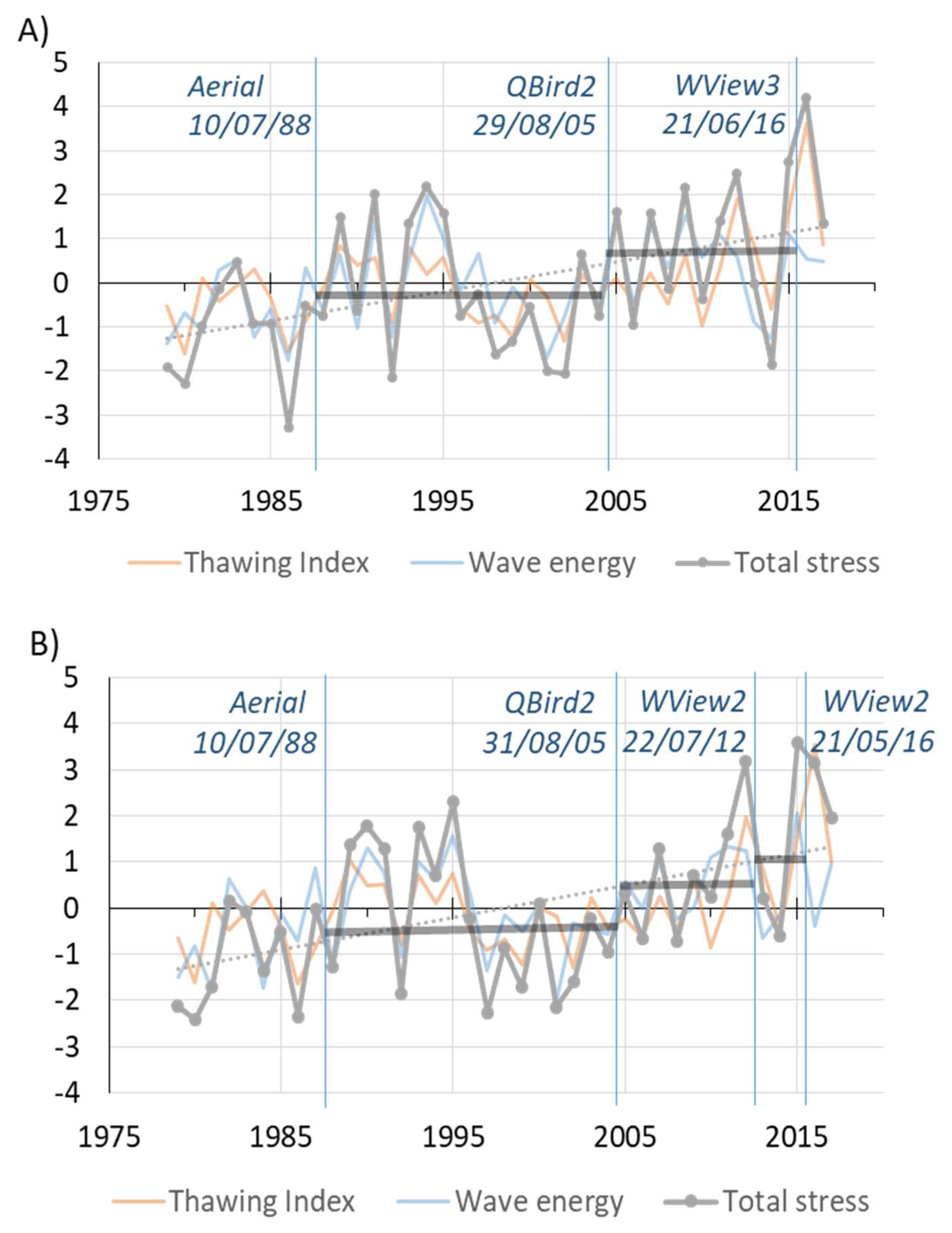
Our results showed a general increase of coastal erosion rates from the 1960s to 2012. This agrees well with estimations of the total hydrometeorological stress on our sites (
Figure 12) and for the Barents-Kara region in general [
73]. The peak erosion rate values typical for 2005–2012 coincided with high hydrometeorological stress [
73]. Still, the subsistent high total stress in 2013–2015 did not result in high retreat rates in this period. The reason is that total stress was low during two previous years. For the 12–16 m terrace this led to a temporary stop in erosion. The energy of the storms of 2015 was spent on the removal of material that had come to the beach in previous years. The thermal factor could also begin to work only after the removal of the thawed sediment by waves. Therefore, despite the high total stress in 2015, the retreat rates for this period in comparison with the rates of 1988–2005 were the same for high terraces and for the 2–4 m laida. That is to say, the higher the shore is, the less resistant it is to changes in hydrometeorological forcing. The rates of retreat of higher shores in a particular year are determined not only by the situation of this year, but also by the combination of wave energy and the thermal factor in previous years.
Before the recent climate change, the Arctic coasts experienced a long, 9–10-month period of conservation when the bluffs and sea were covered by ice and snow [
26,
66]. As a result of sea ice extent decline, autumn storms fell into the ice-free period causing significant retreat. This was especially noticeable in 2005, when the wind-wave energy was even higher than later in 2012 on both Yamal and Ural coasts [
58]. Such increases in wind-wave energy affect all coasts. From the example of the Alaskan coasts, it was found that storm frequency shows the best correlation with erosion rates, contrarily to temperature and precipitation [
73]. On the Ural coast, storm surges of 2009–2010 [
43] provided catastrophic retreat of the laida coasts.
The wind-wave energy is the main factor determining the retreat of the Yamal coast; however, for the Ural coast, both the thermal and wind-wave energy factors are important [
74]. Therefore, the Ural coast turns out to be more vulnerable to the ongoing climatic changes. The summers from 2005 to 2012 were relatively warm, causing active thawing of the coastal bluffs. Positive air temperatures prevailed for about five months [
75].
Generally, within most of the Arctic coasts, a growth of erosion rates was observed since the beginning of the 2000s [
26,
30,
75]. However, periods of active retreat alternate with years of low erosion. Such is the case of Baydaratskaya Bay in 2012–2016, when coastal erosion was even smaller than in the 20th century. The main reason for that was the relatively low wind-wave energy (despite high temperatures). This shows that in spite of the general increase of erosion rates with climate change, this rising trend is imposed by cyclic fluctuations, proved for both the Russian [
21,
25,
43] and Canadian [
67] Arctic.
5.2.3. Human Impact on Coastal Dynamics
As the underwater pipeline crossing of Baydaratskaya Bay was constructed in 2008–2012, human activity could have an impact on the erosion rates of 2005–2012 and 2012–2016 only. Indeed, in 2005–2012 and in 2005–2016, erosion rates increased by up to several times on the Ural and Yamal coast, accordingly. However, this increase coincided with high values of wind-wave energy in 2005–2012 (
Figure 12 and [
26]), that make it challenging to distinguish natural and human-induced processes.
At the same time, clear evidence of the construction’s impact on the spatial distribution of erosion rates can be noted. The most prominent example is the redistribution of the sediment fluxes by cofferdams. In their angles directed towards the longshore sediment flux direction, accumulation starts; as a result, areas that are behind the cofferdams get eroded. On the Ural coasts, this happened to profiles 26–28, originally accumulative and stable, where coastal retreat of 2–8 m/yr happened between 2005 and 2012. The maximum rates of retreat of low laida were caused by the disturbance of the vegetation cover by heavy vehicles. The rest of the coastline did not experience so much technogenic pressure, as the longshore sediment flux is directed to the southeast. Therefore, the erosional coasts were not influenced by the cofferdams’ construction.
On the Yamal coast, the sediment flux near the cofferdams is directed northwards. As a result of enhanced erosion behind the cofferdams, the 6–8 m terrace near profile 7 (
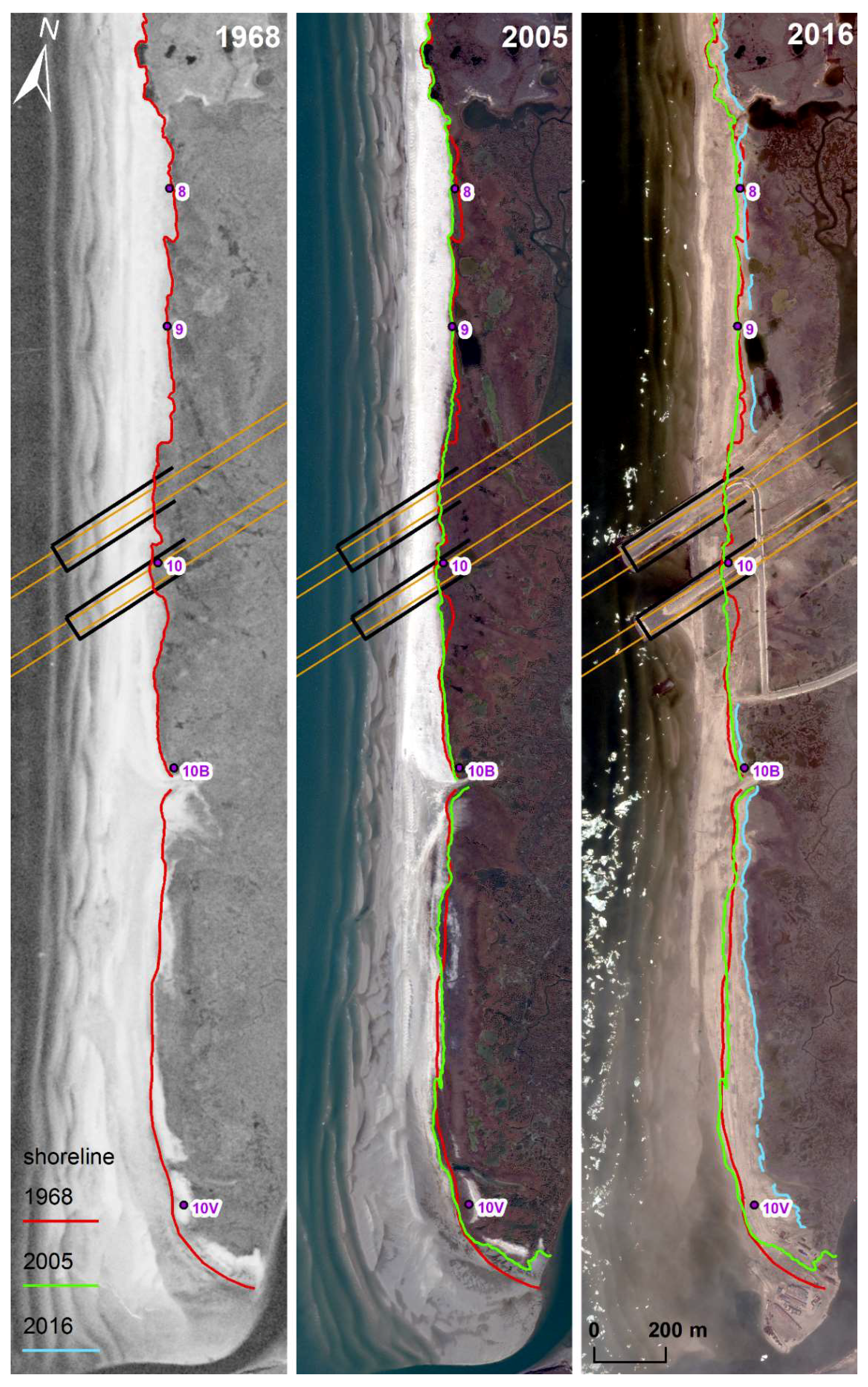
Figure 7) experienced record high retreat rates of more than 3 m/yr from 2005 to 2016, while in the rest of the territory, such an increase was smaller (not more than 2.5 m/yr). Accumulative segments near profiles 8–9, which were previously considered stable, also retreated considerably in 2005–2016 (
Figure 11).
Another example of disturbed sediment balance is dredging around the port at the Yarayakha River mouth at Yamal, seen in satellite images of 2016, which will presumably cause retreat of areas near profiles 10–10V in the years to come. Movement of transport along the beach and on terraces also changes the sediment balance and provokes thermoerosion and thermokarst. In 2005, to the east of the cofferdams, there was evidence of thermokarst along an old road, clearly seen in the satellite image. Disturbance and degradation of vegetation can also cause the disturbance of the thermal regime of solis and the degradation of permafrost and trigger thermoerosion, soil subsidence, and aeolian processes.
6. Conclusions
Remote sensing is a powerful tool in coastal dynamics studies. It is especially relevant in terms of the remoteness and difficult accessibility of Arctic coasts. Despite some of the issues that we faced while working with remotely sensed data, such as relatively low accuracy and a lack of time lapses, we obtained reliable and valid data on coastal dynamics. Based on multi-temporal high resolution aerial and space images and DEMs, we calculated planimetric and volumetric rates of retreat as an integrative estimation of coastal erosion. Remote sensing and field data on geomorphological, lithological, and permafrost conditions allowed us to estimate their contribution to the coastal dynamics.
For the Ural coast, higher erosion rates were typical compared to the Yamal coast. Average rates of retreat of erosional segments of the Ural coast were 1.2 ± 0.15 m/yr and 8.7 ± 1.4 m
3/m/yr from 1964 to 2016; erosional segments of the Yamal coast were eroded with rates of 0.3 ± 0.16 m/yr and 3.7 ± 2.1 m
3/m/yr from 1968 to 2016. Thus, the retreat of the Ural cost was faster and the retreat of the Yamal coast was slower than the average linear erosion rate for the entire Arctic (0.5 m/yr) [
76]. Despite the fact that the key areas were located at the coast of a shallow gulf, the rates of retreat were comparable to those at Western Yamal key sites, at the open coast of the Kara Sea (1.1 m/yr for Kharasavey area [
19] and 1.7 m/yr for Marresale area [
43]). Higher erosion rates at the Ural coast were determined, above all, by its exposure to northerly and north-easterly waves from the open sea. Coastal retreat rates showed significant variability at the Ural key site, while at Yamal, their spatial distribution was uniform. Such local-scale spatial variability is caused by heterogeneous lithology of the Ural key site and the presence of massive ice beds, contrarily to Yamal, where all the bluffs are composed of sand with relatively low ice content.
Remote sensing and field data on geomorphological, lithological, and permafrost conditions allowed us to estimate their contribution to the coastal dynamics. The most intense erosion (up to 9 m/yr) occurred at low laidas with high ice content at the Ural coast in 2005–2012. Lower coastal bluffs tended to be less stable under changing hydrometeorological forcing.
The analysis of temporal variability of coastal retreat rates showed a tendency of their increase since the 1960s associated with climate warming in the Arctic. The temporal variability of the retreat rates is well explained by variability of the thawing index and wave energy flux. We relate sharp acceleration of erosion in 2005–2012 with the increase of wind-wave and thermal impact superimposed on human activity.

 ,
, 


