Abstract
Gaofen-1 02/03/04 satellites, the first civilian high resolution optical operational constellation in China, have Earth observation capabilities with panchromatic/multispectral imaging at 2/8 m resolution. Satellite jitter, the fluctuation of satellite points, has a negative influence on the geometric quality of high-resolution optical satellite imagery. This paper presents an improved jitter detection method based on parallax observation of multispectral sensors for Gaofen-1 02/03/04 satellites, which can eliminate the effect of the relative internal error induced by lens distortion, and accurately estimate the parameters of satellite jitter. The relative internal error is estimated by polynomial modelling and removed from the original parallax image generated by pixel-to-pixel image matching between two bands of images. The accurate relative time-varying error and absolute distortion caused by satellite jitter could be estimated by using the sine function. Three datasets of multispectral images captured by Gaofen-1 02/03/04 satellites were used to conduct the experiments. The results show that the relative system errors in both the across- and along-track directions can be modelled with a quadratic polynomial, and satellite jitter with a frequency of 1.1–1.2 Hz in the across-track direction was detected for the first time. The amplitude of the jitter differed in the three datasets. The largest amplitude, from satellite 04, is 1.3 pixels. The smallest amplitude, from satellite 02, is 0.077 pixels. The reliability and accuracy of the detection results were verified by using two groups of band combinations and ortho-images with a 1 m resolution. The comparison results show that the detection accuracy is improved by approximately 30% using the proposed method.
1. Introduction
Satellite jitter, which is the micro-vibration of satellites, has become one of the most important factors affecting the geometric quality of high-resolution optical satellite imagery [1,2,3,4]. Satellite jitter has been observed in many high-resolution satellites, including QuickBird, Beijing-1, ALOS, Pleiades, ZiYuan1-02C (ZY1-02C), and ZiYuan-3 (ZY-3) [5,6,7,8,9,10,11,12,13]. Satellite jitter of 0.6–0.7 Hz was found during the early in-flight data collection of ZiYuan-3, which caused an internal periodic distortion in both the three-line array camera imagery and multispectral camera imagery [13,14,15,16,17].
To remove the negative effect of jitter on the quality of the images and their products, jitter detection is one of most important steps in ground processing systems as it allows distortion caused by satellite jitter to be corrected [4,18]. Furthermore, jitter detection can also determine the source of satellite jitter. The published methods of jitter detection can be categorized into two classes. One class is based on using imagery to obtain the distortion caused by satellite jitter through using images with parallax observation (such as multispectral imagery, staggered CCD (Charge Coupled Device) images, and stereo image pairs), ortho-images, or linear objects in images [6,7,8,11,12,13,14,15,16,17,19,20,21,22]. The other class is based on attitude sensors to measure the fluctuating attitude [23,24,25]. Table 1 lists the state-of-the-art jitter detection results using these two kinds of methods. Due to higher flexibility, independence, and low cost, jitter detection based on imagery with parallax observation has been widely used with many satellites.

Table 1.
The state-of-the-art jitter detection results and adopted methods.
Gaofen-1 02/03/04 satellites, launched on the 13 March 2018, comprise the first civilian high-resolution optical operational constellation in China. Two identical 2/8 m optical cameras with a panchromatic band and four multispectral bands are installed on each satellite. The four multispectral bands include blue (B1), green (B2), red (B3), and infrared (B4), which are placed parallel to a focal plane with parallax observation. Each band has three sub-CCDs, named CCD1–3, as shown in Figure 1. If the satellites fly smoothly, the coordinate difference of the corresponding points on two different bands in the image is almost fixed, considering the distance between the two bands is very small, and the projection errors caused by topographic relief can be ignored. Otherwise, the coordinate difference will vary with time when satellite jitter exists. Hence, satellite jitter can be detected by analyzing the parallax of multispectral images, which can be applied to the Gaofen-1 02/03/04 satellites.
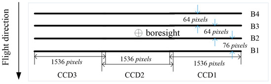
Figure 1.
Diagrammatic sketch of the multispectral camera focal plane of Gaofen-1 02/03/04 satellites.
Jitter detection based on multispectral images was first presented by Teshima and Iwasaki [19] using the level-1B data products of ASTER/SWIR sensor with a pushbroom system of 2048 linear-array detectors of a CCD, which are projected to the map after radiometric calibration and geometric correction. For multi-CCD sensors, level 0 raw image data is used to guarantee the detected results will not be affected by geometric correction and slicing operations [13]. However, the internal distortion, such as lens distortion and CCD deformation in raw images, is a non-negligible factor that will affect the estimation accuracy of satellite jitter, which has not been considered in previous studies. To address this problem, this paper presents an improved jitter detection method that considers the internal distortion for Gaofen-1 02/03/04 satellites. The relative internal distortion between bands was estimated by polynomial modelling and removed from the parallax images, such that the accurate relative time-varying error was obtained, and the jitter distortion was modelled by the sine function. The results of three Gaofen-1 02/03/04 satellite image scenes show the existence of satellite jitter during the early in-flight data collection period, which provided efficient information for in-flight testing.
2. Materials and Methods
Suppose that is the time interval between two bands of scanning of the same ground surface; the relative error, , caused by satellite jitter, can be expressed by the following [3,4]:
where is the absolute distortion caused by satellite jitter.
To reconstruct the satellite jitter using parallax observation of multispectral imagery, the key is to extract and model the relative time-varying errors between two bands. As mentioned above, the relative error between two bands consists of not only the relative time-varying error caused by satellite jitter, but also the relative internal error induced by the camera, such as lens distortion and CCD deformation. Before modeling the relative time-varying error, the relative internal error should be estimated and removed from the relative error. For linear-array pushbroom imaging sensors, the internal distortion varies with the detector number of the CCD (image column number), and the jitter distortion varies with time (image line number), which means these two kinds of errors are orthonormal. The relative internal error could be extracted by analyzing the rules of the relative error change occurring with the image column number of the parallax image, which is generated by image matching. The relative time-varying error would be further modelled after removing the relative internal error from the parallax image.
There are three main steps in the whole workflow of jitter detection for Gaofen-1 02/03/04 satellites using raw multispectral images, as shown in Figure 2. First, the parallax image across and along the track between two bands is generated by pixel-by-pixel image matching after relative radiometric correction. Then, the relative internal error of the parallax imagery is estimated by fitting a polynomial model, with the image sample numbers serving as independent variables and removed from the parallax images. Finally, the relative time-varying error is estimated by calculating the average value of each line in the refined parallax images, such that the absolute jitter distortion could be estimated by a sine function model.
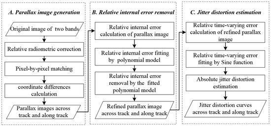
Figure 2.
Workflow of jitter detection of Gaofen-1 02/03/04 satellites using multispectral imagery.
2.1. Parallax Image Generation by Pixel-by-Pixel Matching
To ensure the accuracy of image matching, relative radiometric correction should be conducted to solve the problem of response inconsistency from different detectors, sub-CCDs and bands, through inflight relative radiometric calibration [26].
To ensure the corresponding points distribute evenly and sufficiently, every pixel in the sample direction in each line of the image that has a later imaging time is taken as a detection candidate point. Then, the designed row offset is taken as the initial value, and correlation matching and least-squared matching [27,28] are successively employed to obtain corresponding points with sub-pixel accuracy from the other band image that has an earlier imaging time. Corresponding points whose coordinate differences are beyond the threshold value will be detected and removed.
After image matching, the coordinate differences, , of every point can be calculated. is the coordinate difference in the sample direction, and is the coordinate difference in the line direction minus the designed row offset, where i and j are the sample number and line number of the candidate detection point, respectively. To match failed points, an invalid value, such as −9999, is assigned as the coordinate difference. The DN value of parallax images across the track and along the track, which present coordinate differences in the across- and along-track directions, are assigned by and , respectively.
2.2. Relative Internal Error Removal
The parallax images which represent the coordinate difference consist of not only the relative time-varying error, but also the relative internal error from the camera. Therefore, the relative internal error should be determined and removed before jitter error modelling.
Considering that the relative error between two bands from a linear-array pushbroom camera is a kind of systematic error generally expressed by polynomial model indexed with the CCD detector number [29,30], the relative internal error can be determined by employing a polynomial model index with the image sample number, which means that the error changes with the sample number. To simplify calculations, the average value of each column in the parallax image is calculated, then the polynomial model coefficients are estimated from the averaged value via a least-square fit method. Finally, the refined parallax image is generated by removing the relative systematic error from the original parallax image.
The averaged value of each column of the parallax image is calculated as follows:
where and are the averaged values of column i in the across- and along-track directions, respectively, is the total line number of the parallax image, and is the valid number of corresponding points in column i.
The relative internal error, , could be expressed by the polynomial model, which is a function with the image sample number, i, as an independent variable, as Equation (3) shows:
where and are the coefficients of the polynomial model for the relative internal error in the across- and along-track directions, respectively, and K is the highest degree of the polynomial model, which depends on the error characters, k =1, 2, …, K.
The DN value, , of the refined parallax image in both the across- and along-track directions can be expressed by the following formula:
2.3. Jitter Distortion Estimation
Unlike the relative internal error caused by the camera, error induced by jitter is time-varying. Therefore, the relative error caused by jitter is also time-varying, which means the error changes with the line number. To estimate the jitter distortion, the averaged relative time-varying error of line j is first calculated using the refined parallax image with Equation (5):
where and are the averaged relative time-varying errors of line j in the across- and along-track directions, respectively, m is the total column number of the refined parallax image, and is the valid number of corresponding points in line j.
To reconstruct the jitter, the periodic parameters, including frequency, amplitude and phase of the relative time-varying error in both directions, should be determined. First, the main frequency and amplitude of the relative time-varying error is analyzed by Fourier transform. Then, the sine function is used to fit the relative time-varying error by taking the spectrum analysis result as the initial value; therefore, the accurate frequency, amplitude, and initial phase can be estimated. The relative time-varying error caused by satellite jitter can be expressed by the following formula [31]:
where t is the imaging time of image line j, , is the integral time of each line, , , are the frequency, amplitude, and initial phase of the kth sine component of the relative time-varying error, and N is the total number of sine components.
According to the properties of the resultant vibration, the frequency of jitter distortion is the same as the relative time-varying error [13,16]. If there is only one sine component in the relative time-varying error during a short imaging period, the amplitude of jitter distortion can be calculated using Equation (7) by substituting Equation (6) into Equation (1) [13,22]:
where is the amplitude of jitter distortion, and are the amplitude and frequency of the relative time-varying error, respectively, and is the time interval between two bands of scanning of the same ground surface.
The initial phase, , of jitter distortion can be further calculated using Equation (8) [13,22]:
where presents the remainder of by 2.
Thus, the absolute distortion, , caused by satellite jitter can be expressed as Equation (9):
If the satellite jitter has more than one sine component, every component of jitter distortion can be determined from the corresponding component of the relative time-varying error as for single-frequency satellite jitter. The multiple-frequency distortion caused by satellite jitter can be expressed as Equation (10):
where .
It is noted that Formulas (6–10) are valid for the jitter distortion estimation in both the across- and along-track directions.
3. Results
3.1. Data Description
Three datasets of raw multispectral images captured by three different satellites during the early inflight data collection period were used to conduct the experiments. The basic information regarding the data is shown in Table 2. The raw multispectral images contain three sub-CCD images. The thumbnails of the three images are shown in Figure 3.
Table 2.
Basic information of the datasets.
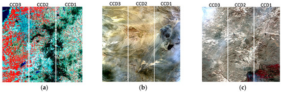
Figure 3.
Thumbnails of (a) Scene A, (b) Scene B, and (c) Scene C (band combination: infrared, green, and blue).
3.2. Jitter Detection Results
Considering that the radiometric character of infrared band images (B4) is very different from that of visible band images (B1, B2, and B3), only B1, B2, and B3 images were used in the experiments.
3.2.1. Results of Band Combination B1–B2
The parallax images of sub-CCD images between B1 and B2 were generated as shown in Figure 4 and Figure 5. It is obvious that the coordinate differences across the track of the three image scenes are periodically varied in correlation with the imaging line, but there is no obvious change along the track for all three sub-CCD images. The amplitude of the variation in Scene C is not as large as those in Scenes A and B. It is indicated that satellite jitter exists with different amplitudes during different imaging periods. Meanwhile, it is noted that the coordinate differences in both directions also change gradually with the sample number from CCD1 to CCD3, which means that there are relative systematic errors between the two bands.
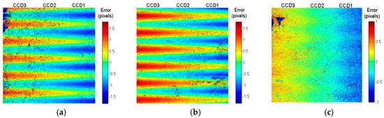
Figure 4.
Parallax images between B1 and B2 across the track of (a) Scene A, (b) Scene B, and (c) Scene C.
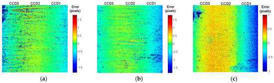
Figure 5.
Parallax images between B1 and B2 along the track (a) Scene A, (b) Scene B, and (c) Scene C.
To avoid the negative effect on the jitter detection, the relative systematic error between these two bands was estimated by the quadratic polynomial model using the method presented in Section 2.2. Figure 6, Figure 7 and Figure 8 show the relative systematic errors and the fitting curves of Scenes A, B, and C. Table 3 lists the estimated polynomial coefficients in both the across and along the track of each scene. It is noted that the relative systematic errors of the three CCDs in the same scene are different, and the relative systematic errors with the same CCD number of the three images differ from each other because they are from three different satellites. Interestingly, the relative systematic error of the three CCDs in both the across- and along-track directions show strong continuity, and a quadratic polynomial model can fit the relative systematic errors from Figure 6, Figure 7 and Figure 8 very well. From Table 3, it is not hard to find that the values of coefficient a2 of the three scenes are lower by 1–2 orders of magnitude compared to the values of coefficient b2, which implies the relative systematic errors across the track are closer to the linear characteristic.
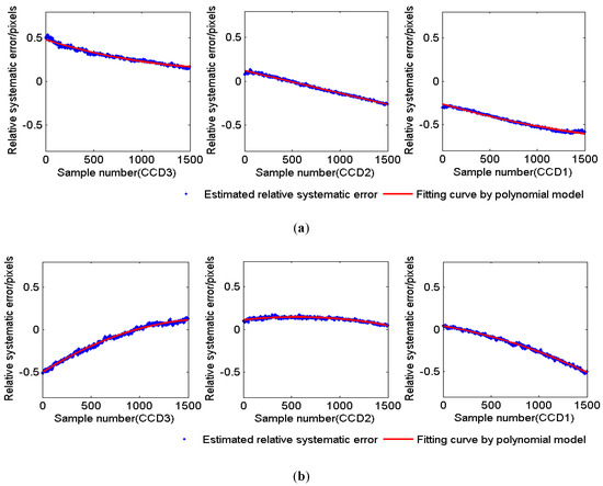
Figure 6.
Relative systematic error between B1 and B2 in Scene A. (a) Across the track and (b) along the track.
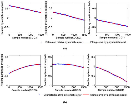
Figure 7.
Relative systematic error between B1 and B2 in Scene B. (a) Across the track and (b) along the track.
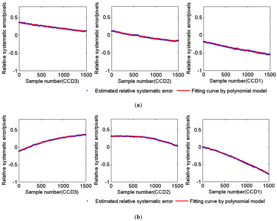
Figure 8.
Relative systematic error between B1 and B2 in Scene C. (a) Across the track and (b) along the track.
Table 3.
Estimated polynomial coefficients of the relative systematic error between B1 and B2.
After removing the relative systematic errors from the original parallax images using the above estimated results, the refined parallax images were generated as shown in Figure 9 and Figure 10. It is obvious that the relative systematic errors in both directions are eliminated. As the geometric difference of each detector was eliminated, the periodicity of the refined parallax images across the track became more obvious. However, it is still difficult to find the time-varying change in the three parallax images along the track, as shown in Figure 10, which means satellite jitter mainly happened in the rolling angle.
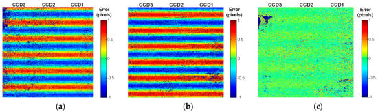
Figure 9.
Parallax images between B1 and B2 across the track of (a) Scene A, (b) Scene B, and (c) Scene C.
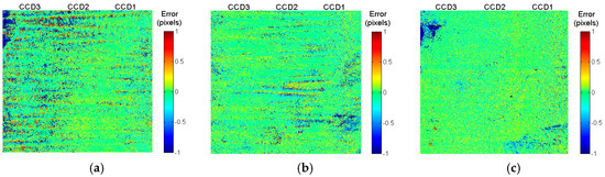
Figure 10.
Parallax images between B1 and B2 along the track of (a) Scene A, (b) Scene B, and (c) Scene C.
Based on the refined parallax image across the track, the averaged relative error of each line in the across-track direction was calculated for these three images. The relative time-varying error curves of the three images, shown in Figure 11, reveal an obvious sine periodicity that changes with time, which is caused by satellite jitter. The estimated frequency, amplitude, and phase of the relative time-varying errors and absolute distortion are listed in Table 4. From the results, the jitter frequencies of the three images suffered are very similar, approximately 1.1–1.2 Hz, and the period equals 0.83–0.91 s, amounting to approximately 830 imaging lines. In addition, the amplitudes of the relative error and absolute distortion are all less than 1.5 pixels. For B1–B2, the in Equation (6) is approximately 0.5, so the absolute distortion is almost twice as big as the relative time-varying error. The biggest distortion caused by satellite jitter is in Scene B, which is 1.2935 pixels in the image space, equaling 10.348 meters in the object space. The smallest distortion is in Scene C, which is 0.0774 pixels in the image space, equaling 0.6192 meters in the object space.
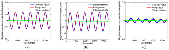
Figure 11.
Relative time-varying errors across the track between B1 and B2 of (a) Scene A, (b) Scene B, and (c) Scene C using refined parallax images.
Table 4.
Detected results using B1–B2 images.
From Figure 11, the frequencies and phases of the fitting results for the three images have strong consistency with the detected results of relative time-varying errors. However, the amplitude of each fitting result has some differences with the corresponding detected result, especially in the positions of peaks and troughs. It is possible that the image matching accuracy was not stable when the differences of the geometric distortion between two bands increased. The other possibility is that the amplitude of satellite jitter is not fixed, so that a single sin function has disadvantages in describing the time-varying error perfectly.
To evaluate accuracy of the fitting results, the residuals of each fitting result were calculated as show in Figure 11. The statistical results of the fitting residuals are listed in Table 5. From the statistical results, the root mean squared errors (RMSEs) of the fitting residuals for the three images are all less than 0.05 pixels, and the absolute values of minimum (Min.) error and maximum (Max.) error are all less than 0.1 pixels. This indicates that the fitting accuracy can meet the requirement of subpixel-accuracy geometric processing and application.
Table 5.
Statistical results of the fitting residuals (unit: pixel).
3.2.2. Results of Band Combination B2–B3
Jitter detection experiments using the B2–B3 band combination were conducted in keeping with the experiments performed using the B1–B2 band combination. Satellite jitter was only found to be the same across the track as the results of B1–B2. The parallax images across the track between B2 and B3 are shown in Figure 12. Table 6 lists the estimated quadratic polynomial coefficients of the relative systematic error across the track between B2 and B3. Compared with the coefficients of the relative systematic error across the track between B1 and B2, the coefficients are all in the same order of magnitude, which means the relative systematic error between B1 and B2 in the across-track direction is also close to the linear characteristic.
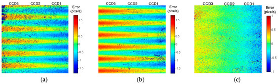
Figure 12.
Parallax images across the track between B2 and B3 of (a) Scene A, (b) Scene B, and (c) Scene C.
Table 6.
Estimated polynomial coefficients of the relative systematic error across the track between B2 and B3.
After removing the relative systematic error, the refined parallax images between B2 and B3 were generated, as shown in Figure 13. The periodic changes with time in the three refined parallax images are more obvious along the image line, and the error in the same line is identical. The frequency, amplitude, and phase of the relative time-varying error and absolute distortion were estimated, as shown in Table 7.
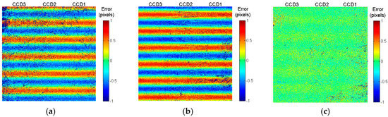
Figure 13.
Refined parallax images across the track between B2 and B3 of (a) Scene A, (b) Scene B, and (c) Scene C.
Table 7.
Detected results using B2–B3 images
4. Discussion
4.1. Consistency Analysis of Results from Two Band Combinations
From the results described above, the detected frequencies of B2–B3 are almost the same as the results of B1–B2. The amplitude differences of the absolute distortion in the three images are all less than 0.02 pixels, which is comparable with the results of B1–B2. It is noted that the relative time-varying errors of B2–B3 are smaller than those of B1–B2 because the distance between B2 and B3 is smaller than that between B1–B2, as Figure 1 shows. The phase differences of the absolute distortion between the two groups of results are less than 0.05 rad.
For a comprehensive assessment, the absolute distortions of each image line, calculated by the sine function using the estimated parameters from the two groups, were compared quantitatively, and the statistical results of the three images are listed in Table 8.
Table 8.
Comparison statistical results (unit: pixel).
From the statistical results, the mean errors of the three images are all less than 0.002 pixels, the RMSEs are all less than 0.05 pixels, and the absolute values of the Min. error and Max. error are all much less than 0.1 pixels. This indicates that the estimated parameters of satellite jitter from the two band combination groups are strongly consistent.
4.2. Evaluation Results Using Ortho-Images
To further evaluate the reliability of the detected results, jitter detection based on ortho-images was conducted. The main steps of jitter distortion detection based on ortho-imagery include dense ground control point (GCP) matching, discrepancy calculation based on geometric imaging modelling [32,33], and image distortion fitting by sine function [15]. In these experiments, ortho-images with a 1 m resolution covering the area of the three test datasets were used. There was a total of 2415, 2069, and 4592 GCPs obtained by image matching using B1 for Scenes A, B, and C, respectively. The discrepancies of the GCPs were calculated with the rational function model (RFM), which was refined by affine modelling to remove the linear system error [34,35]. Due to an insufficient frequency of attitude observations, the RFM cannot absorb the distortion caused by satellite jitter; therefore, the discrepancies of the GCPs in Scenes A and B are periodically varied with the line numbers, as shown in Figure 14a,b. However, the discrepancies of the GCPs in Scene C are randomly distributed with the line numbers, as shown in Figure 14c. It is implied that the image distortion amplitude of Scene C is too small to detect by ortho-images, due to the limitation of the accuracy of the GCP matching between multisource images.
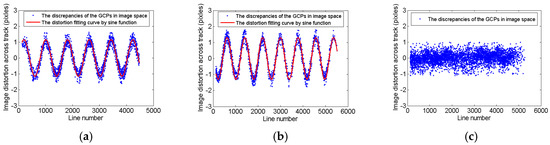
Figure 14.
Image distortion across the track according to the ortho-images of (a) Scene A, (b) Scene B, and (c) Scene C.
The results from sine function-fitting of the absolute distortion of Scenes A and B in the across-track direction according to the ortho-images and the statistical accuracy results compared with the B1–B2 results are listed in Table 9 and Table 10, respectively. The detected results, including frequency, amplitude and phase from the two different methods, are also strongly consistent. The RMSE is considerably smaller than 0.1 pixels and the absolute values of the min. error and max. error are approximately 0.1 pixels.
Table 9.
Fitting results of absolute distortion across the track according to the ortho-images.
Table 10.
Statistical accuracy results (unit: pixel)
Due to the limitation of the accuracy of the GCP matching between multisource images, the accuracy of jitter detection by ortho-imagery is not as good as by multispectral images, especially for satellite jitter with micro-amplitudes, as in Scene C.
4.3. Comparison with the Conventional Method
To analyze the improved effect of the proposed method, the conventional method—which does not remove the relative systematic error based on the original parallax images—was used to estimate the frequency, amplitude, and phase of the relative time-varying error and absolute distortion in the across-track direction, as shown in Table 11. It is noted that the differences between the results of the conventional method and the proposed method are very small. The reason for this phenomenon is that the relative systematic errors between two images in the across the track is antisymmetric, with the center of the CCD as shown in Figure 6, Figure 7 and Figure 8, so the negative effect caused by systematic errors was offset by averaging the relative error of each image line. However, the estimation accuracy of the relative time-varying error by the proposed method is higher than that obtained using the conventional method, as shown in Figure 15 and Table 12. Figure 15 presents the side views of the parallax images between B1 and B2 of the three images. The blue dots and red dots represent the relative errors between B1 and B2 before and after removing relative systematic error, respectively. It is obvious that the red dots are more compact than the blue dots, which means the standard deviation of the red dots is smaller. To evaluate the estimation accuracy of the relative error in each image line, the RMSE of the residuals after averaging the relative errors of corresponding points in the same line was calculated, and the averaged RMSE of the whole image is listed in Table 12. The results show that the detection accuracy is improved by approximately 30% when using the proposed method for these three images.
Table 11.
Results of the conventional method.
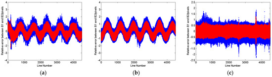
Figure 15.
The side views of the parallax images (blue dots) and refined parallax images (red dots) between B1 and B2 of (a) Scene A, (b) Scene B, and (c) Scene C.
Table 12.
Detection accuracy comparison.
Additionally, the proposed jitter detection method is more effective for non-antisymmetric relative systematic errors in parallax observations. According to the estimated results of the relative systematic errors along the track in Figure 6, Figure 7 and Figure 8, the satellite jitter of Gaofen-1 02/03/04 satellites in the along-track direction could be estimated more accurately using the proposed method than the conventional method if satellite jitter in the pitch angle has occurred. Therefore, the proposed method is more robust, as it would not be affected by the systematic error from the camera.
5. Conclusions
In this paper, an improved jitter detection method based on multispectral imagery for Gaofen-1 02/03/04 satellites was presented. To obtain accurate detection results, the relative systematic error between two bands of images, which is induced by the camera design, was estimated by polynomial modelling in the sample dimension. After removing the relative systematic error, the relative time-varying error and absolute distortion caused by satellite jitter were successively estimated. Three datasets captured by three satellites were used to conduct the experiments. The results show that the relative system error in both the across- and along-track directions can be modelled with a quadratic polynomial. Satellite jitter with a frequency of 1.1–1.2 Hz in the across-track direction was detected in the three datasets using two groups of band combinations for the first time. The amplitude of the jitter differed among different datasets. The largest amplitude, which is from satellite 04, is 1.3 pixels. The smallest amplitude, which is from satellite 02, is 0.077 pixels. Meanwhile, ortho-images with a 1 m resolution were applied to further demonstrate the reliability and accuracy of the results using the proposed method. Compared with the conventional method, the detection accuracy is improved by approximately 30% when the proposed method for the experimental data.
In future work, more datasets with longer imaging duration should be used to analyze the spatiotemporal characteristics of the satellite jitter based on the proposed method, and the effective jitter distortion compensation method based on the detected results for both multispectral and panchromatic imagery should be further investigated.
Author Contributions
Y.Z. conducted the analysis and drafted the paper; M.W. revised the paper; Y.C., L.X, and L.X. conducted the data curation.
Funding
This work was supported in part by the National Natural Science Foundation of China under project 41801382, 91738302, 61825103, and 91838303.
Acknowledgments
The authors would like to thank CRESDA for providing the experimental data.
Conflicts of Interest
The authors declare no conflict of interest.
References
- Roques, S.; Jahan, L.; Rougé, B.; Thiebaut, C. Satellite attitude instability effects on stereo images. In Proceedings of the IEEE International Conference on Acoustics, Speech, and Signal Processing (ICASSP), Montreal, QC, Canada, 17–21 May 2004. [Google Scholar]
- Ayoub, F.; Leprince, S.; Binet, R.; Lewis, K.W.; Aharonson, O.; Avouac, J.P. Influence of Camera Distortions on Satellite Image Registration and Change Detection Applications. In Proceedings of the 2008 IEEE International Geoscience and Remote Sensing Symposium, Boston, MA, USA, 7–11 July 2008. [Google Scholar]
- Iwasaki, A. Detection and Estimation Satellite Attitude Jitter Using Remote Sensing Imagery. In Advances in Spacecraft Technologies; InTech: Rijeka, Croatia, 2011; pp. 257–272. [Google Scholar]
- Tong, X.; Ye, Z.; Xu, Y.; Tang, X.; Liu, S.; Li, L.; Xie, H.; Wang, F.; Li, T.; Hong, Z. Framework of Jitter Detection and Compensation for High Resolution Satellites. Remote Sens. 2014, 6, 3944–3964. [Google Scholar] [CrossRef]
- Robertson, B.C. Rigorous geometric modeling and correction of QuickBird imagery. In Proceedings of the IEEE International Geoscience and Remote Sensing Symposium, Toulouse, France, 21–25 July 2003. [Google Scholar]
- Ran, Q.; Chi, Y.; Wang, Z. Property and removal of jitter in Beijing-1 small satellite panchromatic images. In Proceedings of the International Archives of the Photogrammetry, Remote Sensing and Spatial Information Sciences, Beijing, China, 2008. [Google Scholar]
- Mattson, S.; Boyd, A.; Kirk, R.; Cook, D.A.; Howington-Kraus, E. HiJACK: Correcting spacecraft jitter in HiRISE images of Mars. In Proceedings of the European Planetary Science Congress, Potsdam, Germany, 2009. [Google Scholar]
- Mattson, S.; Robinson, M.; McEwen, A. Early Assessment of Spacecraft Jitter in LROC-NAC. In Proceedings of the 41st Lunar and Planetary Science Conference, Woodlands, TX, USA, 1–5 March 2010. [Google Scholar]
- Takaku, J.; Tadono, T. High Resolution DSM Generation from ALOS Prism-processing Status and Influence of Attitude Fluctuation. In Proceedings of the 2010 IEEE International Geoscience and Remote Sensing Symposium, Honolulu, HI, USA, 25–30 July 2010. [Google Scholar]
- Amberg, V.; Dechoz, C.; Bernard, L.; Greslou, D.; de Lussy, F.; Lebegue, L. In-Flight Attitude Perturbances Estimation: Application to PLEIADES-HR Satellites. In Proceedings of the SPIE Optical Engineering & Applications, International Society for Optics and Photonics, San Diego, CA, USA, 25–29 August 2013. [Google Scholar]
- Jiang, Y.; Zhang, G.; Tang, X.; Li, D.; Huang, W. Detection and Correction of Relative Attitude Errors for ZY1-02C. IEEE Trans. Geosci. Remote Sens. 2014, 52, 7674–7683. [Google Scholar] [CrossRef]
- Sun, T.; Long, H.; Liu, B.; Li, Y. Application of attitude jitter detection based on short-time asynchronous images and compensation methods for Chinese mapping satellite-1. Opt. Express 2015, 23, 1395–1410. [Google Scholar] [CrossRef] [PubMed]
- Tong, X.; Xu, Y.; Ye, Z.; Liu, S.; Tang, X.; Li, L.; Xie, H.; Xie, J. Attitude Oscillation Detection of the ZY-3 Satellite by Using Multispectral Parallax Images. IEEE Trans. Geosci. Remote Sens. 2015, 53, 3522–3534. [Google Scholar] [CrossRef]
- Tong, X.; Li, L.; Liu, S.; Xu, Y.; Ye, Z.; Jin, Y.; Wang, F.; Xie, H. Detection and estimation of ZY-3 three-line array image distortions caused by attitude oscillation. ISPRS J. Photogramm. Remote Sens. 2015, 101, 291–309. [Google Scholar] [CrossRef]
- Liu, S.; Tong, X.; Wang, F.; Sun, W.; Guo, C.; Ye, Z.; Ji, Y. Attitude Jitter Detection Based on Remotely Sensed Images and Dense Ground Controls: A Case Study for Chinese ZY-3 Satellite. IEEE J. Sel. Top. Appl. Earth Obs. Remote Sens. 2016, 9, 5760–5766. [Google Scholar] [CrossRef]
- Wang, M.; Zhu, Y.; Pan, J.; Yong, B.; Zhu, Q. Satellite jitter detection and compensation using multispectral imagery. Remote Sens. Lett. 2016, 7, 513–522. [Google Scholar] [CrossRef]
- Tong, X.; Ye, Z.; Li, L. Detection and Estimation of along-Track Attitude Jitter from Ziyuan-3 three-Line-Array Images Based on Back-Projection Residuals. IEEE Trans. Geosci. Remote Sens. 2017, 55, 4272–4284. [Google Scholar] [CrossRef]
- Tong, X.; Ye, Z.; Liu, S. Essential Technology and Application of Jitter Detection and Compensation for High Resolution Satellite. Acta Geod. Et Cartogr. Sin. 2017, 46, 1500–1508. [Google Scholar]
- Teshima, Y.; Iwasaki, A. Correction of Attitude Fluctuation of Terra Spacecraft Using ASTER/SWIR Imagery with Parallax Observation. IEEE Trans. Geosci. Remote Sens. 2008, 46, 222–227. [Google Scholar] [CrossRef]
- Delvit, J.M.; Greslou, D.; Amberg, V.; Dechoz, C.; de Lussy, F.; Lebegue, L.; Latry, C.; Artigues, S.; Bernard, L. Attitude assessment using Pleiades-HR capabilities. In Proceedings of the International Archives of the Photogrammetry, Remote Sensing and Spatial Information Sciences, Melbourne, Australia, 25 August 2012. [Google Scholar]
- Wang, P.; An, W.; Deng, X.; Yang, Y.; Sheng, W. A jitter compensation method for spaceborne line-array imagery using compressive sampling. Remote Sens. Lett. 2015, 6, 558–567. [Google Scholar] [CrossRef]
- Pan, J.; Che, C.; Zhu, Y.; Wang, M. Satellite jitter estimation and validation using parallax images. Sensors 2017, 17, 83. [Google Scholar] [CrossRef] [PubMed]
- Tang, X.M.; Xie, J.F.; Wang, X.; Jiang, W.S. High-Precision Attitude Post-Processing and Initial Verification for the ZY-3 Satellite. Remote Sens. 2015, 7, 111–134. [Google Scholar] [CrossRef]
- Wang, M.; Zhu, Y.; Jin, S.; Panab, J.; Zhu, Q. Correction of ZY-3 image distortion caused by satellite jitter via virtual steady reimaging using attitude data. ISPRS J. Photogramm. Remote Sens. 2016, 119, 108–123. [Google Scholar] [CrossRef]
- Wang, M.; Fan, C.; Pan, J.; Jina, S.; Chang, X. Image jitter detection and compensation using a high-frequency angular displacement method for Yaogan-26 remote sensing satellite. ISPRS J. Photogramm. Remote Sens. 2017, 130, 32–43. [Google Scholar] [CrossRef]
- Dinguirard, M.; Slater, P.N. Calibration of Space-Multispectral Imaging Sensors: A Review. Remote Sens. Environ. 1999, 68, 194–205. [Google Scholar] [CrossRef]
- Ackermann, F. Digital Image Correlation: Performance and Potential Application in Photogrammetry. Photogramm. Rec. 1984, 11, 429–439. [Google Scholar] [CrossRef]
- Gruen, A. Development and Status of Image Matching in Photogrammetry. Photogramm. Rec. 2012, 27, 36–57. [Google Scholar] [CrossRef]
- Wang, M.; Yang, B.; Hu, F.; Zang, X. On-orbit geometric calibration model and its applications for high-resolution optical satellite imagery. Remote Sens. 2014, 6, 4391–4408. [Google Scholar] [CrossRef]
- Jiang, Y.H.; Zhang, G.; Tang, X.; Li, D.; Wang, T.; Huang, W.; Li, L. Improvement and Assessment of the Geometric Accuracy of Chinese High-Resolution Optical Satellites. IEEE J. Sel. Top. Appl. Earth Obs. Remote Sens. 2015, 8, 4841–4852. [Google Scholar] [CrossRef]
- Hadar, O.; Fisher, M.; Kopeika, N.S. Image Resolution Limits Resulting from Mechanical Vibrations. Part III: Numerical Calculation of Modulation Transfer Function. Opt. Eng. 1992, 31, 581–589. [Google Scholar]
- Toutin, T. Review article: Geometric processing of remote sensing images: Models, algorithms and methods. Int. J. Remote Sens. 2004, 25, 1893–1924. [Google Scholar] [CrossRef]
- Poli, D.; Toutin, T. Review of developments in geometric modelling for high resolution satellite pushbroom sensors. Photogramm. Rec. 2012, 27, 58–73. [Google Scholar] [CrossRef]
- Tao, C.V.; Hu, Y. A comprehensive study of the rational function model for photogrammetric processing. Photogramm. Eng. Remote Sens. 2001, 67, 1347–1358. [Google Scholar]
- Fraser, C.S.; Dial, G.; Grodecki, J. Sensor orientation via RPCs. ISPRS J. Photogramm. Remote. Sens. 2006, 60, 182–194. [Google Scholar] [CrossRef]


© 2018 by the authors. Licensee MDPI, Basel, Switzerland. This article is an open access article distributed under the terms and conditions of the Creative Commons Attribution (CC BY) license (http://creativecommons.org/licenses/by/4.0/).