Figure 1.
An overview of the original global convolutional network (GCN) and boundary refinement (BR) [
15].
Figure 1.
An overview of the original global convolutional network (GCN) and boundary refinement (BR) [
15].
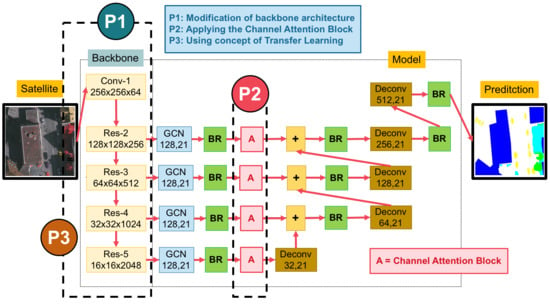
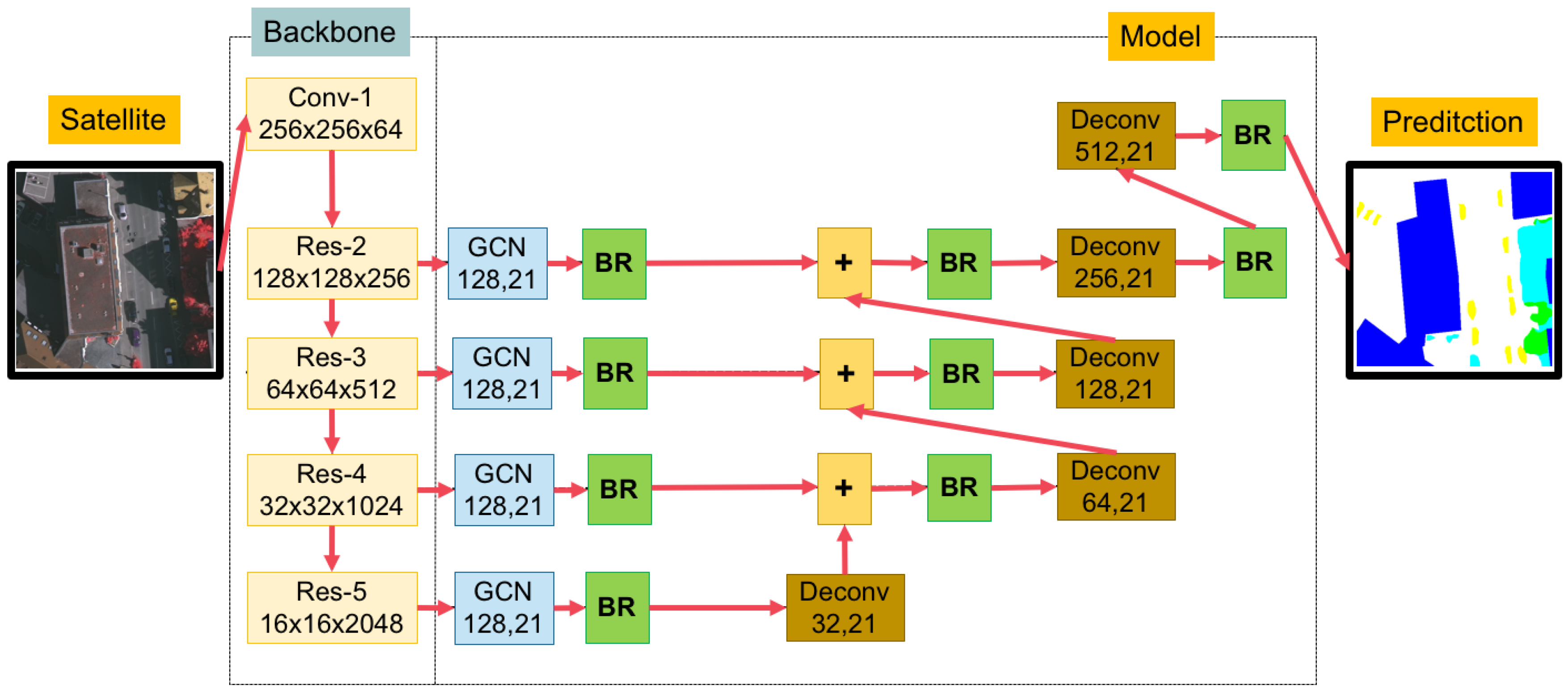
Figure 2.
An overview of our proposed network.
Figure 2.
An overview of our proposed network.
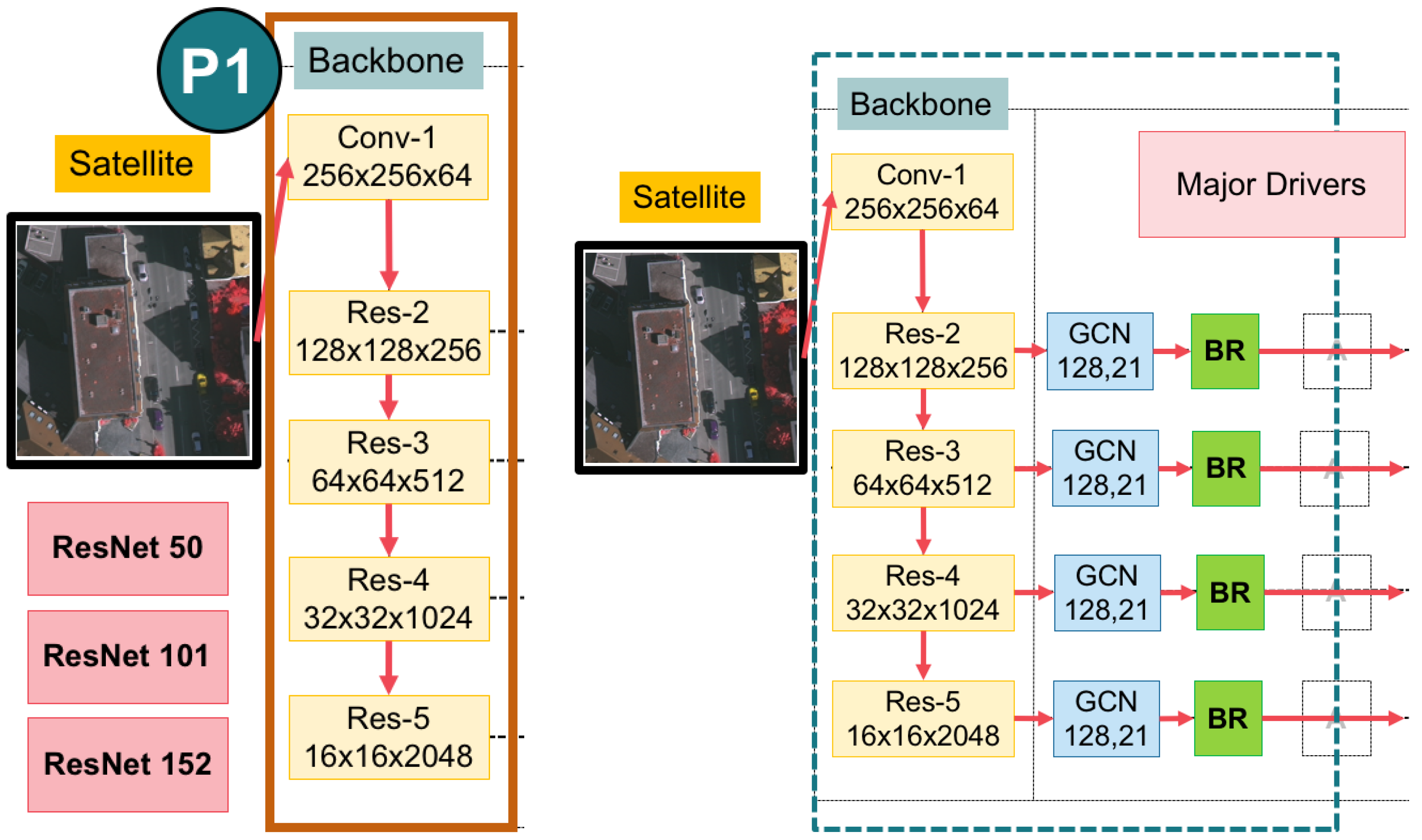
Figure 3.
An overview of the whole backbone pipeline in (
left) the main backbone with varying by ResNet50, ResNet101, and ResNet152; (
right) the major drivers of our main classification network (composed of a global convolutional network (GCN) and a boundary refinement (BR) block [
15]).
Figure 3.
An overview of the whole backbone pipeline in (
left) the main backbone with varying by ResNet50, ResNet101, and ResNet152; (
right) the major drivers of our main classification network (composed of a global convolutional network (GCN) and a boundary refinement (BR) block [
15]).
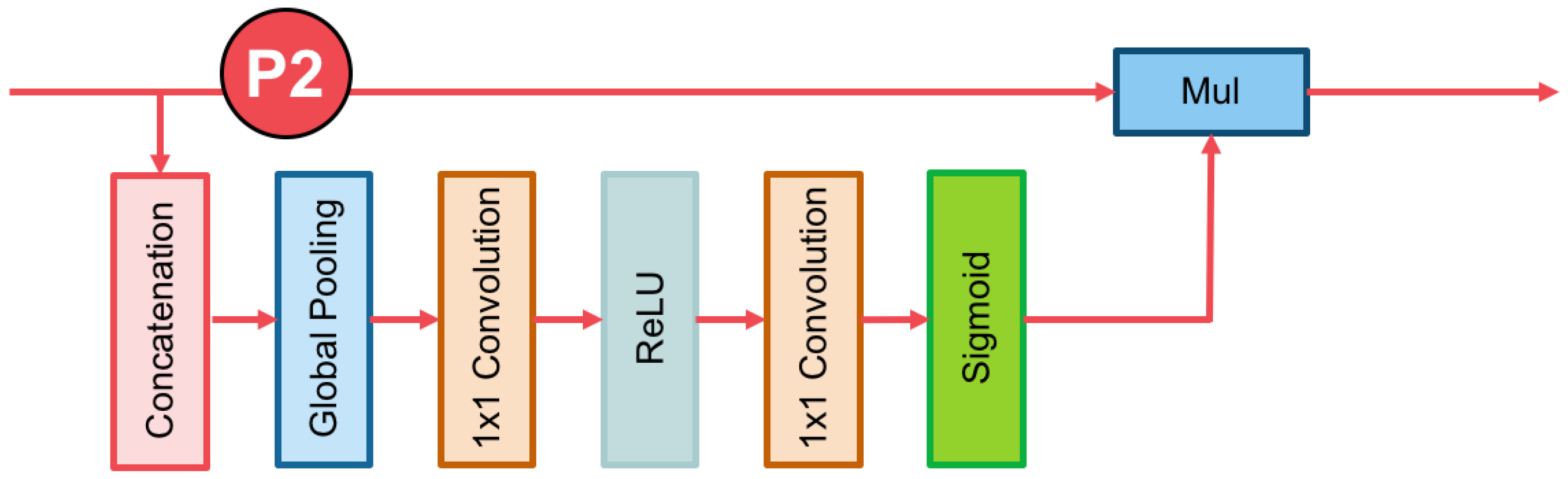
Figure 4.
Components of the channel attention block. The red lines represent the downsample operators, respectively. The red line cannot change the size of feature maps. It is only a path for information passing.
Figure 4.
Components of the channel attention block. The red lines represent the downsample operators, respectively. The red line cannot change the size of feature maps. It is only a path for information passing.
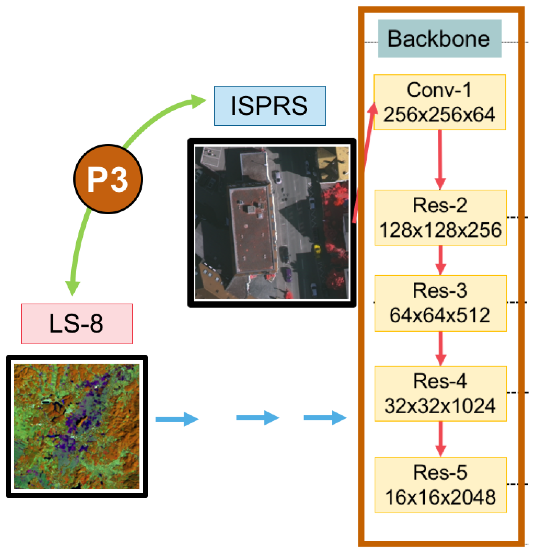
Figure 5.
The domain-specific transfer learning strategy reuses pre-trained weights of models between two datasets—very high (ISPRS) and medium (Landsat-8; LS-8) resolution images.
Figure 5.
The domain-specific transfer learning strategy reuses pre-trained weights of models between two datasets—very high (ISPRS) and medium (Landsat-8; LS-8) resolution images.
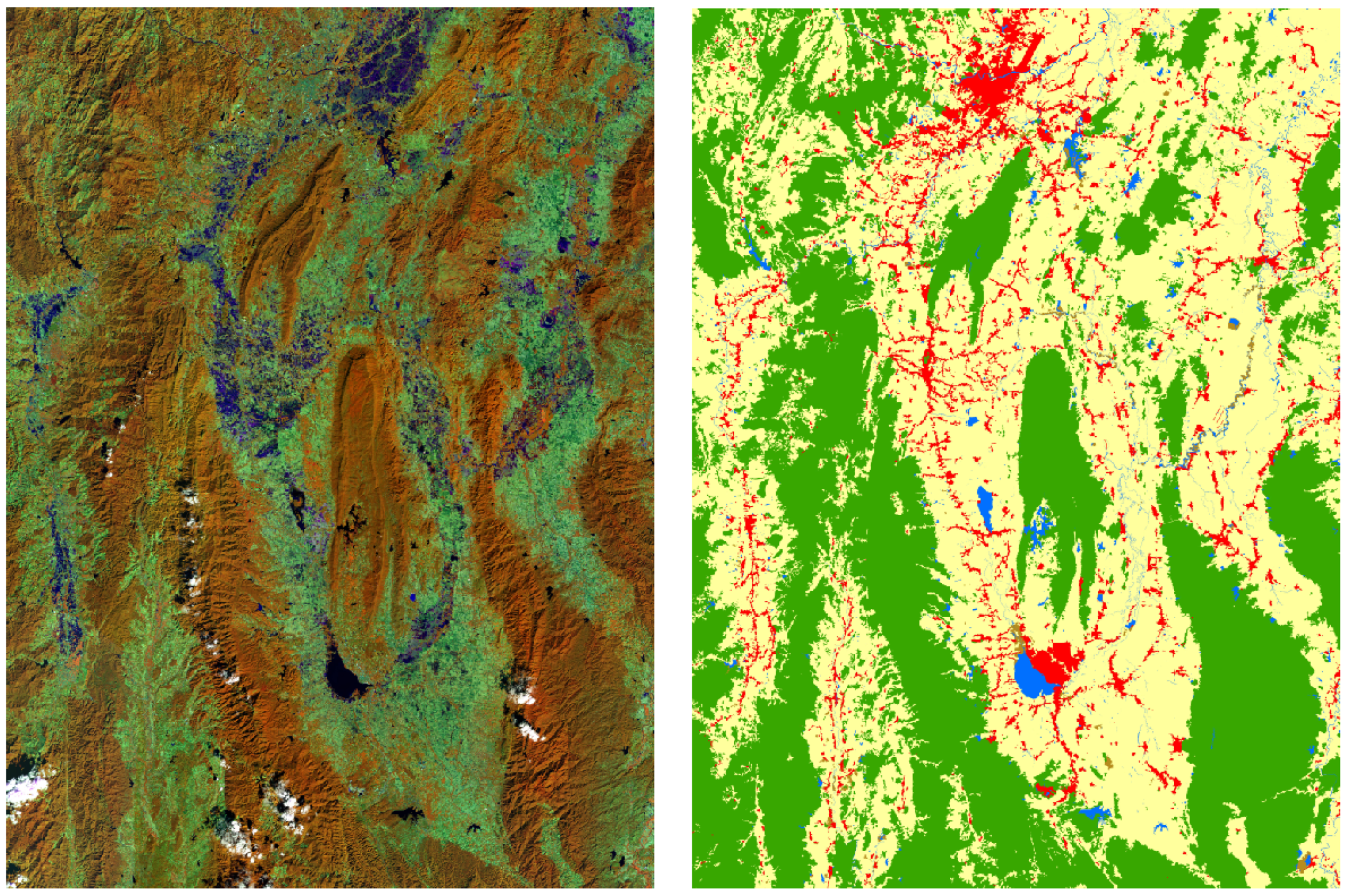
Figure 6.
Sample satellite images from Nan, a province in Thailand (left), and corresponding ground truth (right). The label of medium resolution dataset includes five categories: agriculture (yellow), forest (green), miscellaneous (brown), urban (red), and water (blue).
Figure 6.
Sample satellite images from Nan, a province in Thailand (left), and corresponding ground truth (right). The label of medium resolution dataset includes five categories: agriculture (yellow), forest (green), miscellaneous (brown), urban (red), and water (blue).
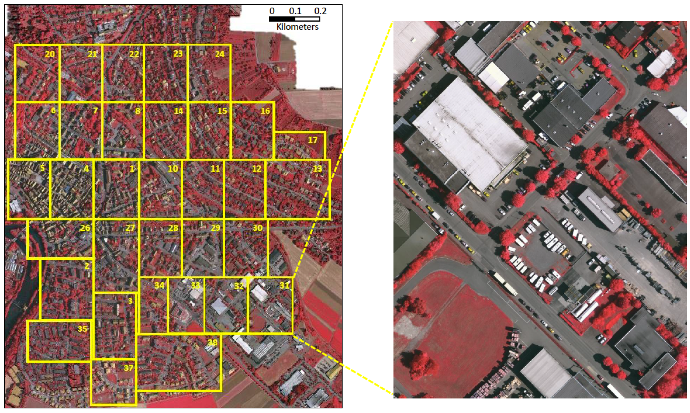
Figure 7.
Overview of the ISPRS 2D Vaihingen Labeling corpus. There are 33 tiles. Numbers in the figure refer to the individual tile flag.
Figure 7.
Overview of the ISPRS 2D Vaihingen Labeling corpus. There are 33 tiles. Numbers in the figure refer to the individual tile flag.
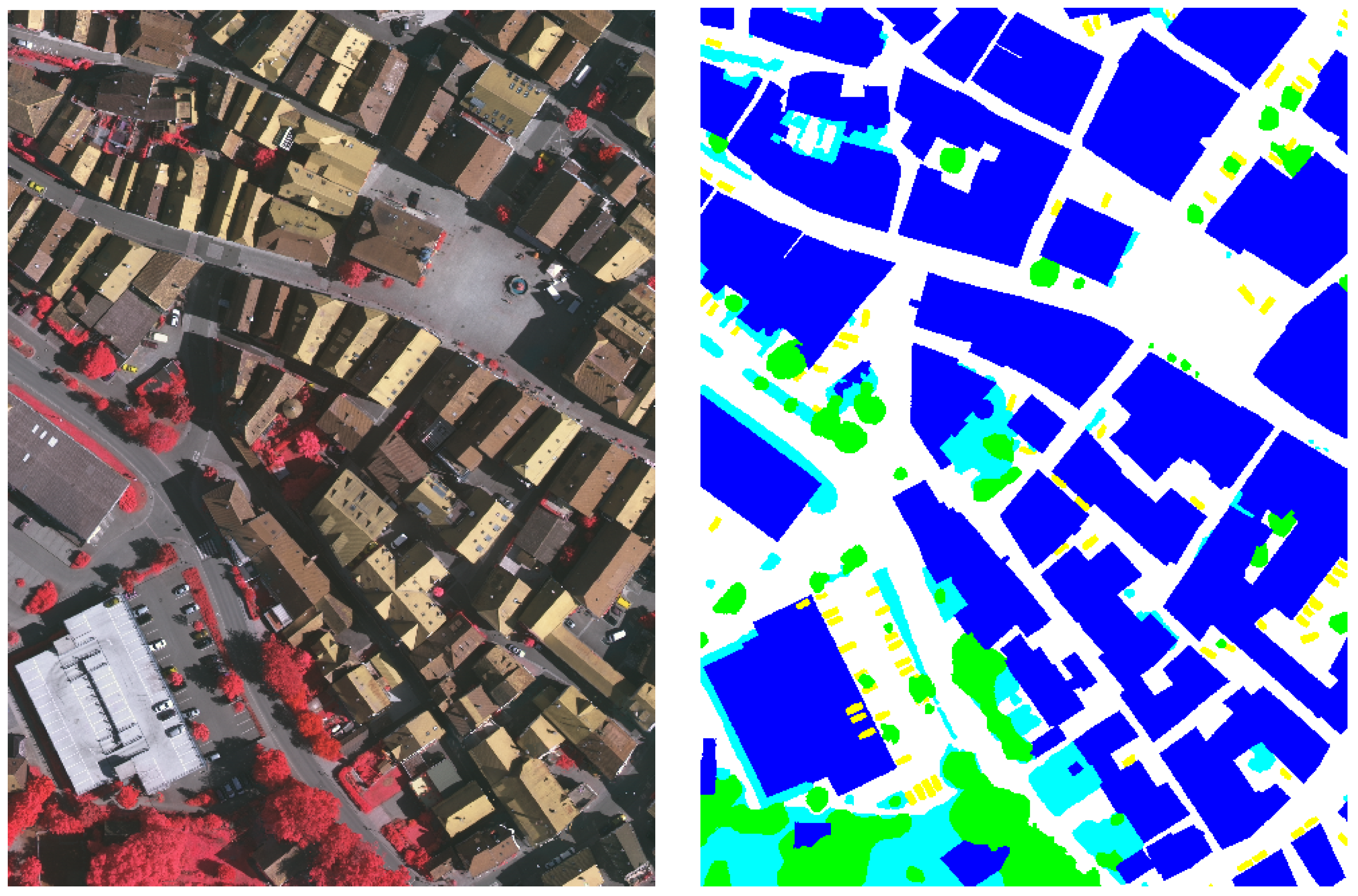
Figure 8.
The sample input tile from
Figure 7 (
left) and corresponding ground truth (
right). The label of the Vaihingen Challenge includes six categories: impervious surface (imp surf, white), building (blue), low vegetation (low veg, cyan), tree (green), car (yellow), and clutter/background (red).
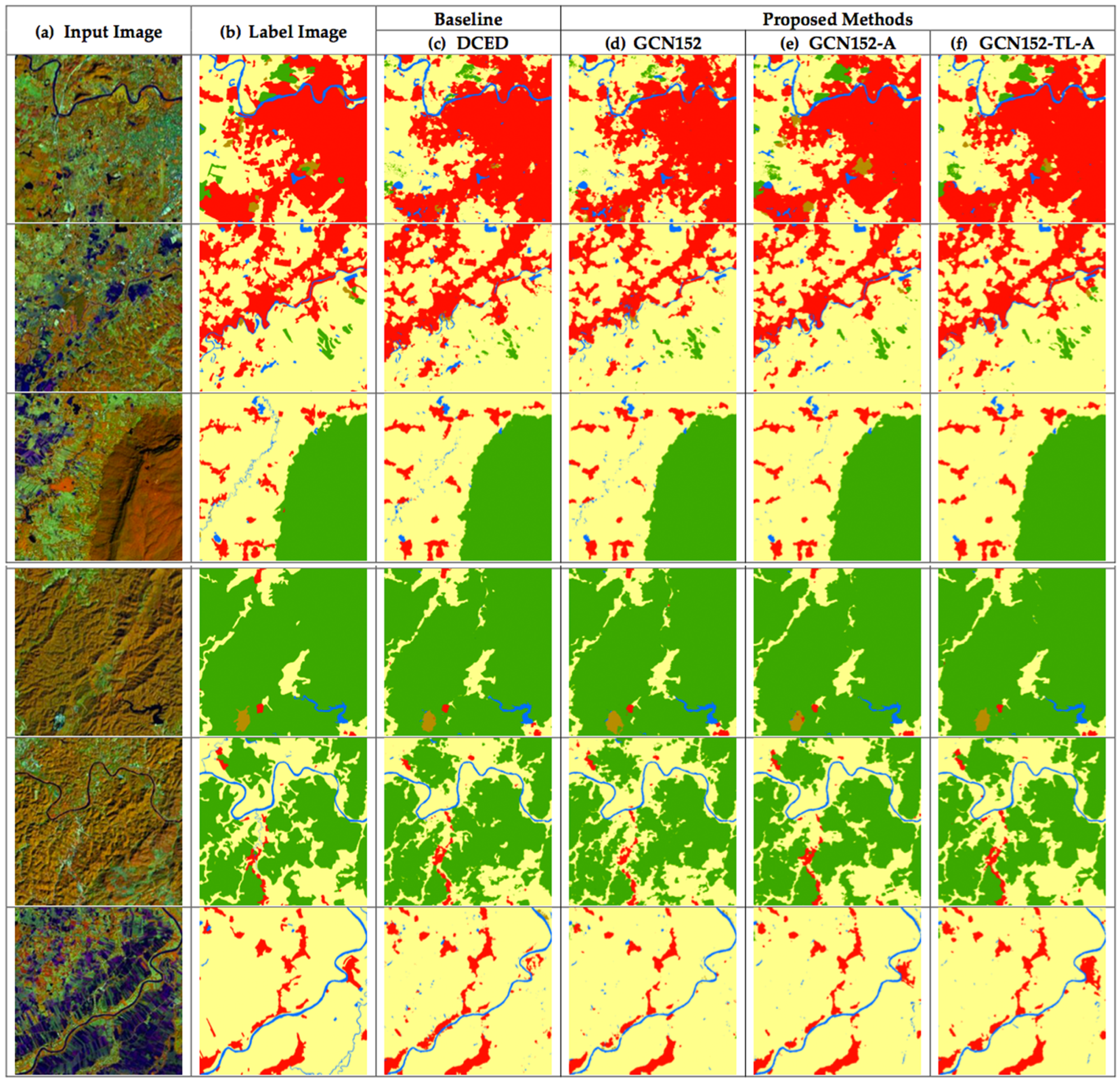
Figure 9.
Six testing sample inputs and output satellite images on Landsat-8 in the Nan province in Thailand, where rows refer to different images. (a) Original input image. (b) Target map (ground truth). (c) Output of Encoder–Decoder (Baseline). (d) Output of GCN152. (e) Output of GCN152-A. and (f) Output of GCN152-TL-A. The label of medium resolution dataset includes five categories: Agriculture (yellow), Forest (green), Miscellaneous (Misc, brown), Urban (red) and Water (blue).
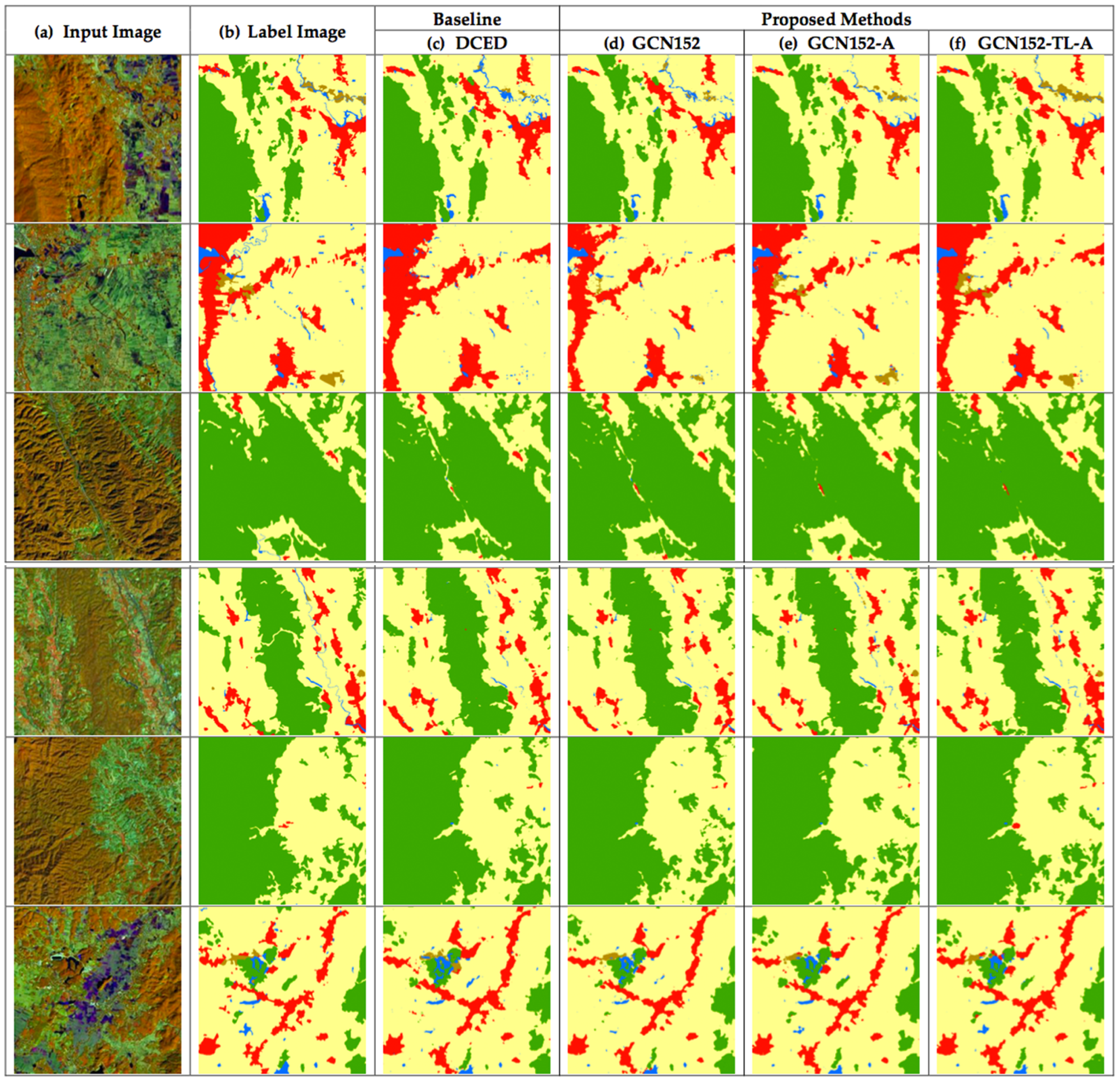
Figure 10.
Six testing sample input and output satellite images on Landsat-8 in Nan in Thailand, where rows refer to different images. (a) Original input image. (b) Target map (ground truth). (c) Output of Encoder–Decoder (Baseline). (d) Output of GCN152. (e) Output of GCN152-A. and (f) Output of GCN152-TL-A. The label of medium resolution dataset includes five categories: Agriculture (yellow), Forest (green), Miscellaneous (Misc, brown), Urban (red) and Water (blue).
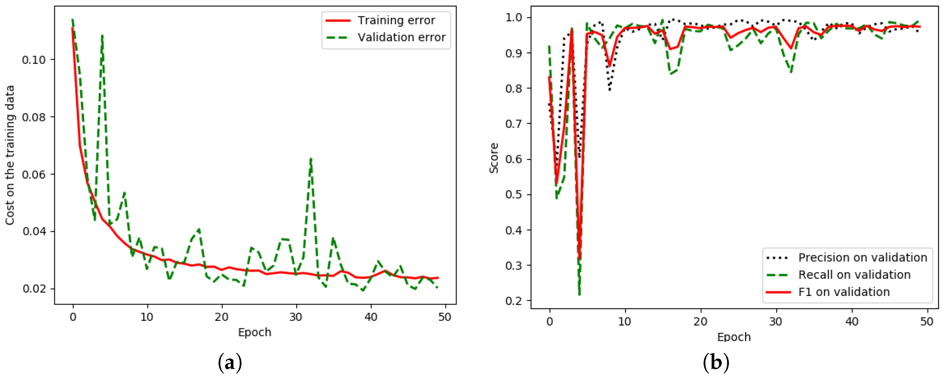
Figure 11.
Iteration plot on Landsat-8 corpus of the proposed technique, GCN152-TL-A; x refers to epochs and y refers to different measures (a) Plot of model loss (cross entropy) on training and validation datasets; (b) performance plot on the validation dataset.
Figure 11.
Iteration plot on Landsat-8 corpus of the proposed technique, GCN152-TL-A; x refers to epochs and y refers to different measures (a) Plot of model loss (cross entropy) on training and validation datasets; (b) performance plot on the validation dataset.
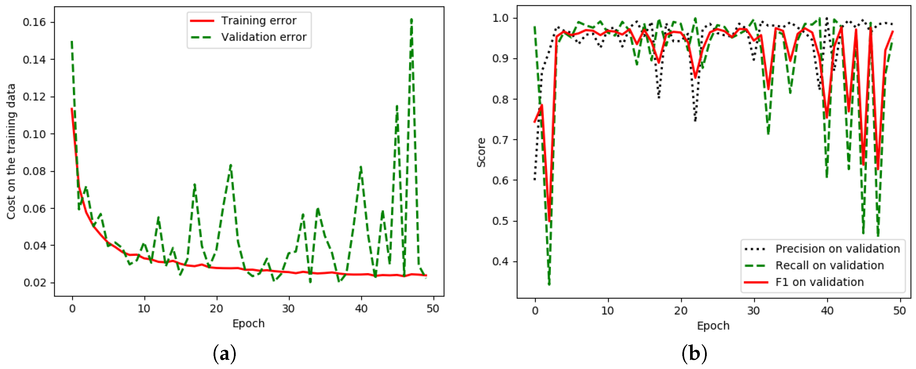
Figure 12.
Iteration plot on the Landsat-8 corpus of the baseline technique, the DCED [
31,
32,
33];
x refers to epochs and
y refers to different measures. (
a) The plot of model loss (cross entropy) on training and validation datasets; (
b) the performance plot on the validation dataset.
Figure 12.
Iteration plot on the Landsat-8 corpus of the baseline technique, the DCED [
31,
32,
33];
x refers to epochs and
y refers to different measures. (
a) The plot of model loss (cross entropy) on training and validation datasets; (
b) the performance plot on the validation dataset.
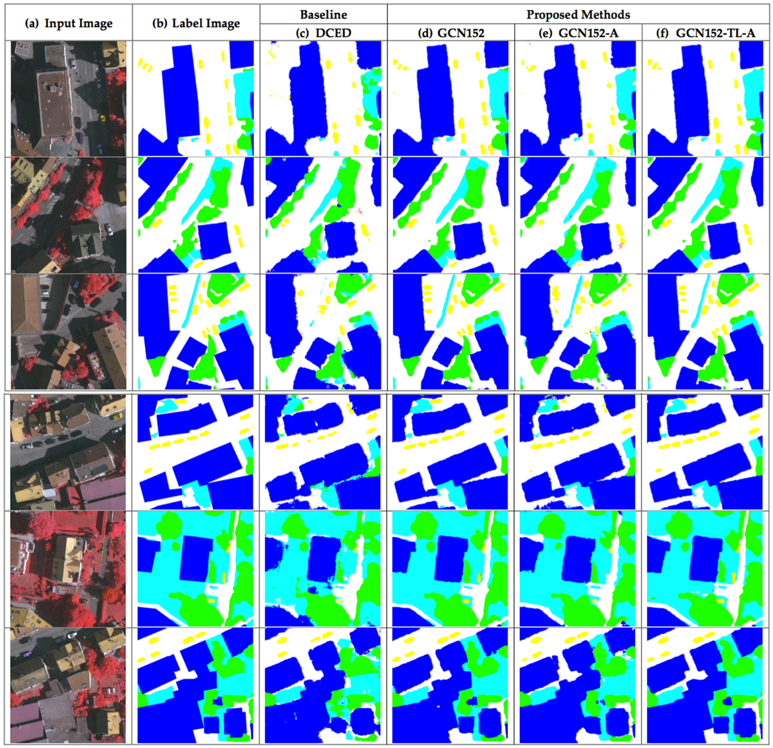
Figure 13.
Six testing sample input and output aerial images on ISPRS Vaihingen Challenge corpus, where rows refer different images. (a) Original input image. (b) Target map (ground truth). (c) Output of Encoder–Decoder (Baseline). (d) Output of GCN152. (e) Output of GCN152-A. and (f) Output of GCN152-TL-A. The label of the Vaihingen Challenge includes six categories: impervious surface (imp surf, white), building (blue), low vegetation (low veg, cyan), tree (green), car (yellow) and clutter/background (red).
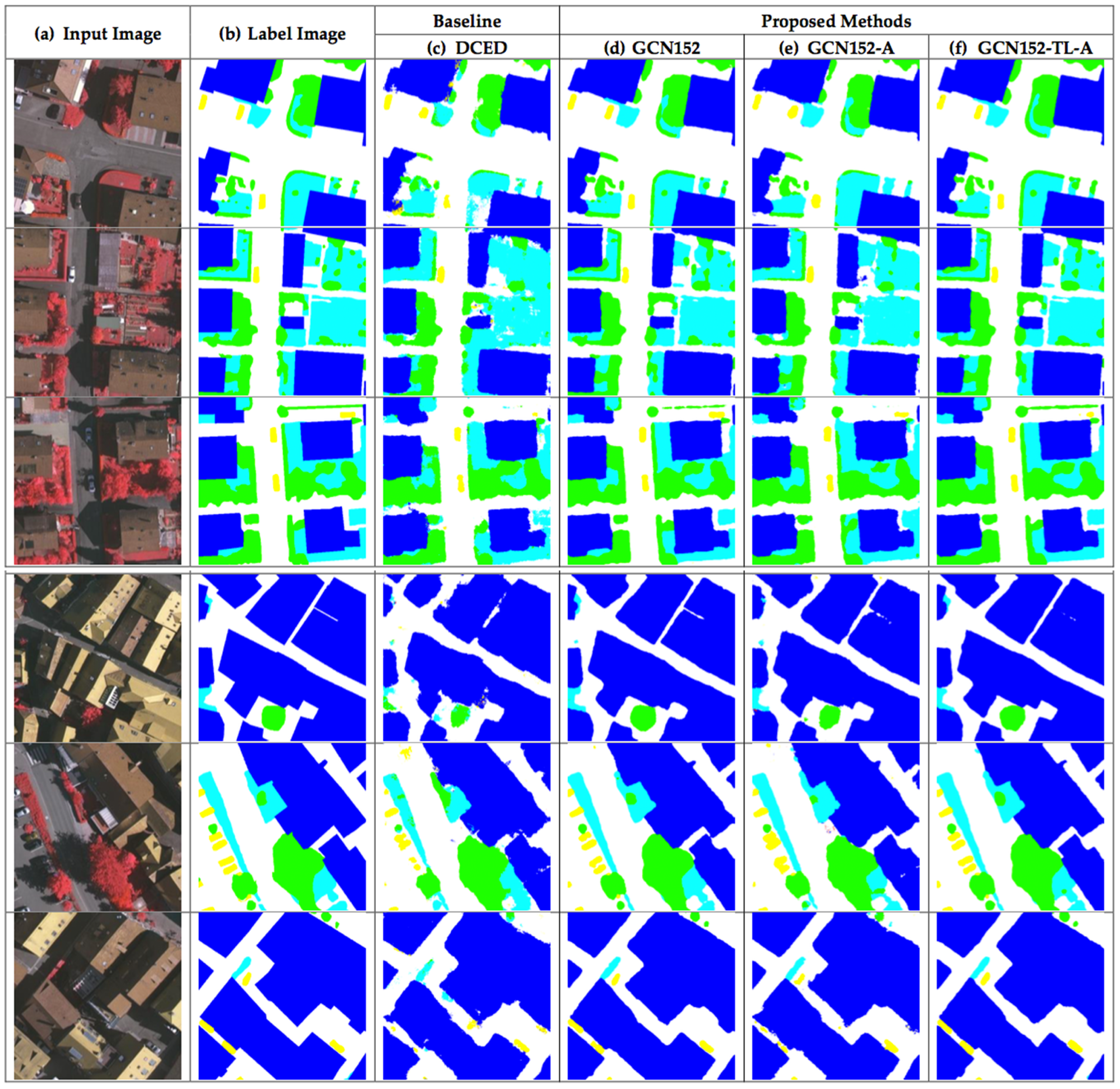
Figure 14.
Six testing sample input and output aerial images on ISPRS Vaihingen Challenge corpus, where rows refer different images. (a) Original input image; (b) Target map (ground truth); (c) Output of Encoder–Decoder (Baseline); (d) Output of GCN152; (e) Output of GCN152-A; and (f) Output of GCN152-TL-A. The label of the Vaihingen Challenge includes six categories: impervious surface (imp surf, white), building (blue), low vegetation (low veg, cyan), tree (green), car (yellow), and clutter/background (red).
Table 1.
Abbreviations on our proposed deep learning methods.
Table 1.
Abbreviations on our proposed deep learning methods.
| Abbreviation | Description |
|---|
| A | Channel Attention Block |
| GCN | Global Convolutional Network |
| GCN50 | Global Convolutional Network with ResNet50 |
| GCN101 | Global Convolutional Network with ResNet101 |
| GCN152 | Global Convolutional Network with ResNet52 |
| TL | Domain-Specific Transfer Learning |
Table 2.
Results of the testing data of the Landsat-8 corpus between baseline and five variations of our proposed techniques in terms of , , , and .
Table 2.
Results of the testing data of the Landsat-8 corpus between baseline and five variations of our proposed techniques in terms of , , , and .
| | Pretrained | Backbone | Model | | | | |
|---|
| Baseline | - | - | DCED [31,32,33] | 0.6137 | 0.7209 | 0.6495 | 0.5384 |
| | - | Res50 | GCN [15] | 0.6678 | 0.7333 | 0.6847 | 0.5734 |
| | - | Res101 | GCN | 0.6899 | 0.8031 | 0.7290 | 0.6154 |
| Proposed Method | - | Res152 | GCN | 0.7115 | 0.8131 | 0.7563 | 0.6364 |
| | - | Res152 | GCN-A | 0.7997 | 0.7937 | 0.7897 | 0.6726 |
| | TL | Res152 | GCN-A | 0.8293 | 0.8476 | 0.8275 | 0.7178 |
Table 3.
Results of the testing data of Landsat-8 corpus between each class with our proposed techniques in terms of .
Table 3.
Results of the testing data of Landsat-8 corpus between each class with our proposed techniques in terms of .
| | Model | Agriculture | Forest | Misc | Urban | Water |
|---|
| Baseline | DCED [31,32,33] | 0.9616 | 0.7472 | 0.0976 | 0.7878 | 0.4742 |
| | GCN50 [15] | 0.9407 | 0.8258 | 0.1470 | 0.8828 | 0.5426 |
| | GCN101 | 0.9677 | 0.8806 | 0.2561 | 0.7971 | 0.5480 |
| Proposed Method | GCN152 | 0.9780 | 0.8444 | 0.4256 | 0.7158 | 0.5937 |
| | GCN152-A | 0.9502 | 0.9118 | 0.6689 | 0.8675 | 0.6001 |
| | GCN152-TL-A | 0.9781 | 0.8472 | 0.8732 | 0.7988 | 0.6493 |
Table 4.
Results of the testing data of the ISPRS 2D semantic labeling challenge corpus between the baseline and five variations of our proposed techniques in terms of , , , and .
Table 4.
Results of the testing data of the ISPRS 2D semantic labeling challenge corpus between the baseline and five variations of our proposed techniques in terms of , , , and .
| | Pretrained | Backbone | Model | | | | |
|---|
| Baseline | - | - | DCED [31,32,33] | 0.7519 | 0.7925 | 0.7693 | 0.8651 |
| | - | Res50 | GCN [15] | 0.7636 | 0.7917 | 0.776 | 0.8776 |
| | - | Res101 | GCN | 0.7713 | 0.8059 | 0.7862 | 0.8972 |
| Proposed Method | - | Res152 | GCN | 0.7736 | 0.8021 | 0.7864 | 0.8977 |
| | - | Res152 | GCN-A | 0.7847 | 0.7961 | 0.7902 | 0.9057 |
| | TL | Res152 | GCN-A | 0.7888 | 0.8001 | 0.7942 | 0.9123 |
Table 5.
Results of the testing data of ISPRS Vaihingen Challenge corpus between each class with our proposed techniques in terms of .
Table 5.
Results of the testing data of ISPRS Vaihingen Challenge corpus between each class with our proposed techniques in terms of .
| | Model | IS | Buildings | LV | Tree | Car |
|---|
| Baseline | DCED [31,32,33] | 0.9590 | 0.9778 | 0.9108 | 0.9805 | 0.6832 |
| | GCN50 [15] | 0.9595 | 0.9628 | 0.9403 | 0.9896 | 0.7292 |
| | GCN101 | 0.9652 | 0.9827 | 0.9615 | 0.9797 | 0.7387 |
| Proposed Method | GCN152 | 0.9543 | 0.9962 | 0.9445 | 0.9754 | 0.7710 |
| | GCN152-A | 0.9614 | 0.9865 | 0.9554 | 0.9871 | 0.8181 |
| | GCN152-TL-A | 0.9664 | 0.9700 | 0.9499 | 0.9901 | 0.8567 |

 ,
, 


