Article

Non-Rigid Vehicle-Borne LiDAR-Assisted Aerotriangulation

1
School of Geodesy and Geomatics, Wuhan University, Wuhan 430079, China
2
Anhui Huadian Engineering Consultating&Design CO., LTD, Anhui 230022, China
3
School of Remote Sensing and Information Engineering, Wuhan University, Wuhan 430079, China
4
Department of Geography and GeoInformation Sciences, College of Science, George Mason University, Fairfax, VA 22030-4444, USA
*
Author to whom correspondence should be addressed.
Remote Sens. 2019, 11(10), 1188; https://doi.org/10.3390/rs11101188
Submission received: 2 April 2019 / Revised: 13 May 2019 / Accepted: 15 May 2019 / Published: 18 May 2019
(This article belongs to the Special Issue Point Cloud Processing in Remote Sensing)

Abstract

:
VLS (Vehicle-borne Laser Scanning) can easily scan the road surface in the close range with high density. UAV (Unmanned Aerial Vehicle) can capture a wider range of ground images. Due to the complementary features of platforms of VLS and UAV, combining the two methods becomes a more effective method of data acquisition. In this paper, a non-rigid method for the aerotriangulation of UAV images assisted by a vehicle-borne light detection and ranging (LiDAR) point cloud is proposed, which greatly reduces the number of control points and improves the automation. We convert the LiDAR point cloud-assisted aerotriangulation into a registration problem between two point clouds, which does not require complicated feature extraction and match between point cloud and images. Compared with the iterative closest point (ICP) algorithm, this method can address the non-rigid image distortion with a more rigorous adjustment model and a higher accuracy of aerotriangulation. The experimental results show that the constraint of the LiDAR point cloud ensures the high accuracy of the aerotriangulation, even in the absence of control points. The root-mean-square error (RMSE) of the checkpoints on the x, y, and z axes are 0.118 m, 0.163 m, and 0.084m, respectively, which verifies the reliability of the proposed method. As a necessary condition for joint mapping, the research based on VLS and UAV images in uncontrolled circumstances will greatly improve the efficiency of joint mapping and reduce its cost.

Graphical Abstract

1. Introduction

Under the global trend of intelligent development, intelligent transportation construction is in full swing. The acquisition of high-precision road geometry information is the foundation of intelligent transportation construction. Aerotriangulation of UAV (Unmanned Aerial Vehicle) images is an important way to obtain three-dimensional (3D) geometric information. However, the control points need to be manually deployed and measured in order to obtain high-precision results, resulting in a low degree of automation. Although the presence of a global positioning system (GPS) and an inertial measurement unit (IMU) has reduced the number of ground control points (GCPs), it is difficult to obtain GPS/IMU data with higher accuracy, which makes it difficult to meet application requirements in the absence of control points [1,2]. Phantom 4 RTK, produced by DJI, appeared on the market in 2018. The accuracy of the uncontrolled mapping technology based on RTK has reached 5 cm, but its point cloud elevation accuracy and density are still lower than those of VLS (Vehicle-borne Laser Scanning) [3].With the heterogeneity of the sensors, how to use the information obtained by multiple sensors to form an intelligent service system and avoid the insufficiency of limited data sources is the current research direction [4].
The emergence of light detection and ranging (LiDAR) provides a new technological approach for sparsely controlled aerotriangulation. Compared with photogrammetry, LiDAR can quickly obtain the three-dimensional coordinates and reflection intensity information of the object surface, which is called LiDAR point cloud. In particular, the LiDAR point cloud acquired by a vehicle-borne laser scanning system has the characteristics of both high density and high accuracy. However, this technology also has its disadvantages, i.e., it cannot directly obtain surface texture information [5,6,7]. On the basis of the complementarity between LiDAR and photogrammetry, the vehicle-borne LiDAR point cloud data is employed as a control to constrain the aerotriangulation of UAV images, thereby achieving high-precision aerotriangulation under sparse control [8,9].
In this paper, the road point cloud acquired by a vehicle laser scanning system and the UAV images is utilized, and a point cloud-assisted aerotriangulation method based on non-rigid registration is proposed, which can achieve higher-precision orientation elements under sparse control. In the platform, the UAV is professional, and the type is M600. Its flight time without load is 60 minutes, and its maximum horizontal flight speed is 18 m/s in the windless environment.
The method firstly uses GPS/IMU data for rough absolute orientation, and generates a 3D feature point cloud of images in the geodetic coordinate system by aerotriangulation [10]. LiDAR point cloud is then used to correct this point set point-by-point. The corrections are combined with the bundle block adjustment as a virtual observation, and then new orientation elements and a 3D feature point cloud from the image are solved. Finally, the above-mentioned point-by-point correction and joint adjustment process are continuously repeated until the distance correction between the two point sets is small enough or the maximum number of iterations is reached, then the iteration ends. While the relative positions between images will be changed, the external orientation elements of each image are corrected by different parameters. Therefore, it is called a non-rigid method.
Our key contributions are summarized as follows: we propose a vehicle-borne LiDAR point cloud-assisted aerotriangulation method based on non-rigid registration. By adding virtual observations to the bundle block adjustment, the high-precision orientation elements are calculated under sparse control. This process is simple and easy without complicated feature extraction and matching operations. Compared with the point cloud-assisted aerotriangulation method based on iterative closest point (ICP) rigid registration, this method corrects the non-rigid distortion of the 3D feature point cloud. Moreover, there is no need to generate a dense point cloud, speeding up non-rigid registration and avoiding the effects of noise in dense point clouds.
The remainder of the paper is organized as follows: We begin with a review of related work in Section 2. The main steps of our method are described in detail in Section 3. Our experiment results are discussed in Section 4, and conclusions are drawn in the final section.

2. Related Work

The LiDAR-assisted aerotriangulation process is essentially a problem of applying the registration of LiDAR point clouds and multi-images to aerotriangulation in order to improve the localization accuracy of the images. Common methods include the following two:
One is a feature-based point cloud-assisted aerotriangulation method. This method finds similar features directly between LiDAR point cloud and aerial images and establishes a direct mapping relationship between point clouds and images. Commonly used features are mainly corner features, line features, and planar features [11,12]. Habib et al. [13,14] used the same line features and plane features on LiDAR point cloud and images to calculate the transformation parameters between the two types of data and to perform self-calibration of the camera while improving the accuracy of image positioning. However, the process requires manual extraction of the line segments or planar features in the LiDAR point cloud, so automation level is low. To improve automation, Zhang et al. [15] automatically extracted corner features, and then used the initial orientation element to project the corner features of the airborne LiDAR point cloud onto the related image and search the same corner features on the image. The corner points of the LiDAR point cloud served as GCPs, while the corresponding corner points on the images served as image points. Finally, the bundle block adjustment improved the positioning accuracy of the images. Additionally, Sheng et al. [16] comprehensively analyzed the direction and position information of line features and proposed a registration method based on line feature vectors. The authors stated the line features’ vector description method in detail, and deduced the mathematical model of the registration. Cui et al. [4] did similar research but focused on aligning the panoramic image and the LiDAR point cloud using a line-based registration method. Yang et al. [17] estimated the external orientation element parameters by extracting and matching the building outlines on the LiDAR point cloud and images.
Another method is a point cloud-assisted aerotriangulation method based on point set registration. The method firstly generates the 3D feature point cloud of the aerial images by computer vision [18,19] or photogrammetry [20]. Then, the 3D feature point cloud is registered with the LiDAR point cloud, and the registration results are involved in aerotriangulation. Thus, the LiDAR point cloud-assisted aerotriangulation is converted into a registration between the LiDAR point cloud and the 3D feature point cloud. The registration of two point sets is generally divided into two processes—rough registration and fine registration. Rough registration is a process of rough absolute orientation of the 3D feature point cloud, which is roughly aligned to the LiDAR point cloud, to initially prepare for the fine registration. GPS/IMU data, for instance, is often used for rough absolute orientation. Under the absence of GPS/IMU data, Abayowa et al. [21] achieved rough alignment through feature extraction and match. The ICP algorithm [22] is often used to minimize the global error between a 3D feature point cloud and LiDAR point cloud in fine registration. Chen et al. [23] improved the ICP algorithm by using the constraint of relative motion threshold. The ICP registration process, however, does not consider the consequences of non-rigid distortions appearing in both the images and the generated 3D point cloud. In current related research work, reducing the impact of non-rigid distortion to the precision is only applied to simple scenes, such as close-range photogrammetry. Li et al. [24] and Zheng et al. [25], given the distance between the 3D feature point cloud and the LiDAR point cloud, established an error equation and added it to the bundle block adjustment for iterative calculation. They handled the problem of non-rigid distortion between the LiDAR point cloud and images, however, whether this method is suitable for large scenes such as aerial images still needs to be verified. Swart et al. [26] performed ICP on a 3D feature point cloud on the basis of continuous segmentation of the trajectory, and then applied it to bundle block adjustment. Although this method reduces the non-rigid distortion in large scene data such as aerial images, the accuracy is not high and other methods are required to be combined to improve the performance.
The first method is not suitable for terrain without obvious features, but the matching process of this method is complicated. When the features are extracted from the LiDAR point cloud, the error is relatively large with lots of mismatches. The difficulty lies in the automatic extraction and matching of the characteristics between the LiDAR point cloud and the images, and the degree of automation is not high enough. In contrast, the second method avoids finding similar features between images and LiDAR point cloud and is able to be used in the absence of obvious features. Additionally, the operation is simpler, the applicability is stronger, and the reliability is higher in the actual application process. However, strong non-rigid distortion exists when point cloud-assisted aerotriangulation based on ICP rigid registration is used in a big scene, resulting in low accuracy of aerotriangulation [19,27].This paper proposed a point cloud assisted aerotriangulation method based on non-rigid registration to solve this problem. Our approach can be used in large-scale scene photogrammetry, and greatly decreases the number of GCPs while increasing the automation of aerotriangulation.

3. Methodology

Compared with traditional aerotriangulation, we propose a LiDAR point cloud-assisted aerotriangulation method based on non-rigid registration and make full use of the fact that the LiDAR point cloud has comprehensive 3D coordinate information. We add virtual observations to the bundle block adjustment, that is, we take the LiDAR point cloud as a constraint to participate in the aerotriangulation. We aim to correct the non-rigid distortion of the 3D feature point cloud and improve the image localization accuracy. The flow chart of this method is comprehensively shown in Figure 1. Our method mainly includes the following key processes:
(1) Aerotriangulation of UAV images: during aerotriangulation, GPS and IMU data are employed during the rough absolute orientation to generate a 3D feature point cloud of images in the geodetic coordinate system, which is roughly aligned to the LiDAR point cloud.
(2) LiDAR point cloud constraints: The LiDAR point cloud performs point-by-point correction on the 3D feature point cloud. The correction parameters are combined with the bundle block adjustment to solve the new exterior orientation elements and generate a 3D feature point cloud, which takes the most computation.
(3) Tolerance threshold check-out: Check the distance between the 3D feature point cloud and the corresponding LiDAR plane. If the distance correction is sufficiently small between two iterations or the maximum number of iterations is reached, the accuracy evaluation process is entered, otherwise step (2) is continued.

3.1. UAV Image Aerotriangulation

The premise of the LiDAR point cloud-assisted aerotriangulation is to unify the coordinates of the UAV images and the LiDAR point cloud so that the 3D feature point cloud is roughly aligned with the LiDAR point cloud. The main coordinate reference system for this process is shown in Figure 2, where S 1 and S 2 are image space coordinate systems, L is the laser scanner coordinate system, and W is the geodetic coordinate system. For the laser scanning system, the position and attitude parameters of the laser scanner are obtained by GPS and an inertial navigation system (INS), and then the 3D coordinates of the ground laser point in the geodetic coordinate system can be solved according to the angle and the round-trip time of the laser beam emission. For the UAV images, the 3D feature point cloud in the geodetic coordinate system can be obtained through aerotriangulation. Thus, the LiDAR point cloud-assisted aerotriangulation is turned into the problem of two point-sets registration in the geodetic coordinate system.
On the basis of the basic principles of aerotriangulation, we use the self-calibration bundle block adjustment [28] as the basic adjustment model to generate the 3D feature point cloud in the geodetic coordinate system. The self-calibration bundle block adjustment is based on the Collinearity Equations [19] as a mathematical model for adjustment. The expression is as followings:
{ x x 0 Δ x = f a 1 ( X A X S ) + b 1 ( Y A Y S ) + c 1 ( Z A Z S ) a 3 ( X A X S ) + b 3 ( Y A Y S ) + c 3 ( Z A Z S ) y y 0 Δ y = f a 2 ( X A X S ) + b 2 ( Y A Y S ) + c 2 ( Z A Z S ) a 3 ( X A X S ) + b 3 ( Y A Y S ) + c 3 ( Z A Z S )
In the above expression, ( x 0 , y 0 ) are the coordinates of the projection center on the image plane, f is the focal length, ( X A , Y A , Z A ) are the coordinates of the object point, ( X s , Y s , Z s ) are the projection center coordinate parameters, and a i , b i , c i are the cosine value of the image attitude angles. Δ x and Δ y represent lens distortion parameters, expressed as Equation (2):
{ Δ x = ( x x 0 ) ( k 1 r 2 + k 2 r 4 ) + p 1 [ r 2 + 2 ( x x 0 ) 2 ] + 2 p 2 ( x x 0 ) ( y y 0 ) Δ y = ( y y 0 ) ( k 1 r 2 + k 2 r 4 ) + p 2 [ r 2 + 2 ( y y 0 ) 2 ] + 2 p 1 ( x x 0 ) ( y y 0 ) r = ( x x 0 ) 2 + ( y y 0 ) 2
In the above formula, ( k 1 , k 2 ) represent the radial distortion parameters, and ( p 1 , p 2 ) are the tangential distortion parameters.
By expanding the Collinearity Equation using the Taylor series to obtain the error equation, we then employ the camera orientation elements and lens distortion as virtual observations by assigning appropriate weights. If the ground control point coordinates are also treated as weighted observations, then we get a self-calibration bundle block adjustment. It can be expressed as the following equations:
{ V x , y = A x , y   Δ t + B x , y   Δ P + C x , y   Δ X N + D x , y   Δ c + E x , y   Δ k       L x , y V N = Δ X N     L N V c = Δ c     L c V k = Δ k     L k
When V x , y = [ V x , V y ] T is the residual vector of image-point observations ( x , y ) , V N represents the error correction vector of the control point coordinates, V c   and   V k represent the error correction vectors of the virtual observation equations corresponding to the interior parameters and the lens distortion parameters. The correction of exterior orientation parameters could be represented by Δ t = [ Δ X s , Δ Y s , Δ Z s , Δ φ , Δ ω , Δ k ] T , where Δ P = [ Δ X , Δ Y , Δ Z ] T is the correction of object point coordinates, Δ X N represents the correction of the coordinates of the control points, Δ c represents the correction of the interior orientation parameters, and Δ k = [ Δ k 1 , Δ k 2 , Δ p 1 , Δ p 2 ] T represents the correction of the lens distortion parameters. A x , y , B x , y , C x , y , D x , y , and E x , y are coefficient matrices, respectively. We define L x , y = [ x ( x ) , y ( y ) ] T , where x denotes the measurement value of the coordinates of the image point and ( x ) denotes the approximate value of the coordinate of the image point. L N , L c , and L k are the corresponding constant items, separately.

3.2. Non-Rigid Vehicle-Borne LiDAR Point-Assisted Aerotriangulation

Due to the poor quality of GPS, the 3D feature point cloud generated by the aerotriangulation is not very accurate—there is an apparent performance gap in both the position and the shape against the LiDAR point cloud. In this paper, the high-precision 3D coordinates of the LiDAR point cloud are treated as constraints to correct the coordinates of the 3D feature point cloud. We combine the correction parameters as virtual observations into the self-calibration bundle block adjustment to calculate new exterior orientation elements. The distance between the 3D feature point cloud and the LiDAR point cloud is recurrently getting smaller and smaller in iteration, so that the image positioning accuracy is continuously improved.
The premise of using the LiDAR point cloud as a constraint is to find the correspondence point between the 3D feature point cloud and the LiDAR point cloud. The LiDAR point cloud density is sparse and thin, therefore the constraining method of the nearest point is not perfect, so we prefer to search the corresponding plane of the 3D feature point cloud on the LiDAR point cloud [29] and use the distance from the point to the corresponding plane as the constraint condition. The specific process of searching for a corresponding plane is described as follows: Firstly, the point-to-point nearest neighbor search method is used to search for the closest point P 0 ( X 0 , Y 0 , Z 0 ) of the 3D feature point cloud P ( X , Y , Z ) on the LiDAR point cloud. In this process, we use k-d tree [30,31,32] to organize the point cloud and speed up the search efficiency for the nearest point. Fit the P 0 and its neighboring point as a plane PL , set any point in the plane as P X ( X , Y , Z ) , then the PL plane can be expressed as Formula (4). Where ( a , b , c , d ) are the parameters of the fitted plane equation.
a X + b Y + c Z + d = 0
Although the position represented by the 3D feature point cloud P cannot be exactly found on the LiDAR point cloud, it is generally assumed that P is on the LiDAR point cloud surface, as shown in Figure 3. Therefore, the constraint of the LiDAR point cloud is actually the process of continuously reducing the distance between the 3D feature point cloud P and the LiDAR point cloud surface. Distance between P and LiDAR surface PL is expressed by formula (5):
D = a X p + b Y p + c Z p + d 0
Taylor series expansion is performed on the above Equation (5) to obtain the error Equation (6):
V P = D X p Δ X p + D Y p Δ Y p + D Z p Δ Z p ( D D 0 )
Equation (6) is then changed to matrix forms and it can be expressed as:
V P = N Δ P L P
where N = [ D X p   , D Y p , D Z p ] , ΔP = Δ P = [ Δ X p , Δ X p , Δ Z p ] T indicates the correction of the generated 3D feature point cloud and L P = D D 0 is a constant term of the error equation.
Compared with the traditional self-calibration bundle block adjustment, the LiDAR point cloud-assisted bundle block adjustment adds a cost function (7) to the adjustment formula (3). This formula evaluates the distance between the 3D feature point cloud and the LiDAR point cloud. The coordinates of the 3D feature point cloud are adjusted by the non-uniform transformation parameters. It means that the adjustment model we proposed can eliminate the non-rigid deformation between the LiDAR point cloud and the 3D feature point cloud. In this paper, the error equation of the LiDAR point cloud-assisted bundle block adjustment is shown as Equation (8), and then the external orientation elements of the images are calculated. Among them, W x , y , W P , W N , W c , W k , are corresponding weights.
{ V x , y = A x , y Δ t + B x , y Δ P + C x , y Δ X N + D x , y Δ c + E x , y   Δ k    L x , y W x , y V P = N Δ P    L P W P V N = Δ X N    L N W N V c = Δ c    L c W C V k = Δ k    L k W k
Expressed in matrix form as:
[ V x , y V P V N V c V k ] = [ A x , y B x , y C x , y D x , y E x , y · N · · · · · E 1 · · · · · E 2 · · · · · E 3 ] [ Δ t Δ P Δ X N Δ c Δ k ] ] [ L x , y L P L N L c L k ]
V   =   M   Δ     L
In Equation (9), E 1 , E 2 , E 3 are unit matrixes. Equation (10) is an abbreviation of Equation (9).
It should be noted that due to the limitations of LiDAR point cloud resolution and the complexity of ground conditions, it is difficult to assess the distance between the 3D feature point cloud and the LiDAR point cloud plane. For example, a 3D feature point that falls on a rough area of the LiDAR point cloud (such as a road edge) may lie on a nearby plane. Figure 4 shows the case where the flat region and the rough region are fitted to a plane. It is obviously that the fitting residual of the flat region is smaller than in the rough region. That means the distance between the 3D feature point and the LiDAR point cloud of the flat region is more reliable. Therefore, we propose that only the 3D feature points that lie in the flat areas of the LiDAR point cloud are constrained and participate in adjustment. This paper evaluates whether the 3D feature point P lies on the flat area by calculating the average distance dis between each point of the fitting plane and the fitting plane. The expression of the distance dis is expressed by Equation (11).
d i s = d 1 2 + d 2 2 + + d n 2 n
Among them, d = { d 1 , d 2 , , d n } denotes the distance between the LiDAR point and its fitting plane. Given a threshold τ , LiDAR points with dis < τ are considered as points on a flat area.
According to our method presented above, it is obviously that the vehicle-borne LiDAR point cloud assisted bundle block adjustment is a continuous iterative process and the iterative processing we designed is as follows:
(1) Find 3D feature points in a flat area and determine their corresponding planes in the vehicle-borne LiDAR point cloud.
(2) Establish the error function and normal function described as Equation (10). Each 3D feature points is corrected point by point.
(3) Solve the equations to get unknown parameter corrections. In this process, the unit-weighted root mean square ( RMS 0 ) is used to evaluate the registration quality. Unit-weighted RMS 0 is defined as:
R M S 0 = V T W V n t
In the above formula, n is the number of observations and t is the number of unknown parameters.
(4) Check RMS 0 and the parameter correction. If it is less than the tolerance, go to step five. Otherwise, repeat steps two to four with the new value of the parameters.
(5) Check the distance DRMS (Distance Root Mean Square) between the 3D feature points and the corresponding LiDAR plane. If the difference in DRMS between the two iterations is small enough or the maximum number of iterations is reached, continue to the accuracy evaluation process; otherwise, jump to step one. DRMS is defined as in Equation (13):
D R M S = i N p d ( P i , Q i ) 2 N p
Here, P i represents the 3D feature points of the flat region, N p is the total number of 3D feature points, and Q i expresses the LiDAR plane corresponding to P i .

4. Experiment and Result Discussion

4.1. Experimental Data

The experimental data set includes UAV images, the vehicle-borne laser point cloud, and three control points. To determine the effectiveness of our method, 17 checkpoints are collected to determine the effectiveness of our method. The data set covers an area of 1.3 km × 1.3 km in Wuhan, Hubei Province, China. The UAV’s flying altitude is about 320 m. There are 10 strips and 245 images. The Endlap is about 80%, and the Sidelap is about 50%. The vehicle-borne LiDAR point cloud cover the same road area. Essential preprocessing must be done before aerotriangulation. However the preprocessing stage is not what we mainly focused on. Thus, here we assume that the preprocessing of the vehicle-borne LiDAR point cloud, including noise filtering and registration, is finished. The detailed information of the optical images is shown in Table 1, and the details of the vehicle-borne LiDAR point cloud are shown in Table 2.
The UAV camera location and image overlap degree are shown in Figure 5.
The distribution of control points and checkpoints is shown in Figure 6a. Red dots indicate the distribution of control points, yellow dots indicate the distribution of checkpoints, and the bottom image is the orthographic image. The vehicle-borne LiDAR point cloud is shown in Figure 6b.
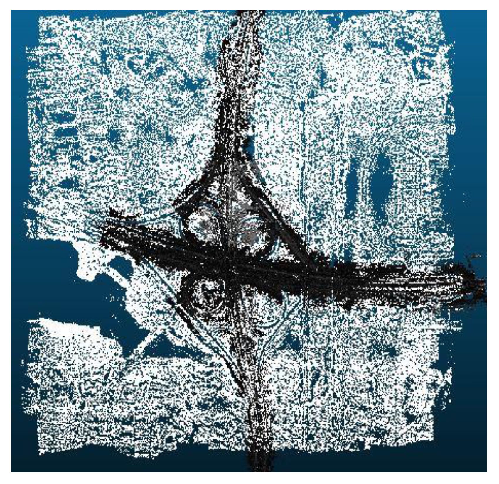
The 3D feature point cloud under the geodetic coordinate system is obtained by aerotriangulation to roughly align with the LiDAR point cloud. The LiDAR point cloud and the 3D feature point cloud are superimposed, as shown in Figure 7. It is clear that there are non-rigid distortions in the 3D feature point cloud. Through the vehicle-borne LiDAR point cloud’s restraint effect on the 3D feature point cloud, the distance between the 3D feature point cloud and the LiDAR point cloud is continuously reduced, until the two point clouds are aligned gradually and a higher image positioning accuracy is obtained.

4.2. Quantitative Evaluation

We use the checkpoints to evaluate the accuracy. The measured ground truth checkpoints are compared with the 3D feature points generated from the bundle block adjustment and constrained by the vehicle-borne LiDAR. The RMSE of the checkpoints are statistically calculated during each iteration. It can be seen from Figure 8 that during the loop iteration process, the RMSE of the checkpoint continuously decreases until convergence, which reflects the effectiveness of the vehicle-borne LiDAR point cloud constraint in this paper.
Table 3 illustrates the error of each ground check point before and after the vehicle-borne LiDAR point cloud constrained aerotriangulation. Before the LiDAR point cloud constraint, the RMSE of the checkpoints on the x, y, and z axes are 0.140 m, 0.193 m, and 1.341 m, respectively. The RMSE of the checkpoints on the x, y, and z axes after the LiDAR point cloud constraint are 0.118 m, 0.163 m, and 0.084 m, respectively, and the maximum residual is less than 0.3 m. On the basis of the comparison, it is proved that, in the case of rare control, the image positioning accuracy can be improved by the constraint of the LiDAR point cloud and the accuracy requirement can be satisfied.

4.3. Visual Quality Evaluation

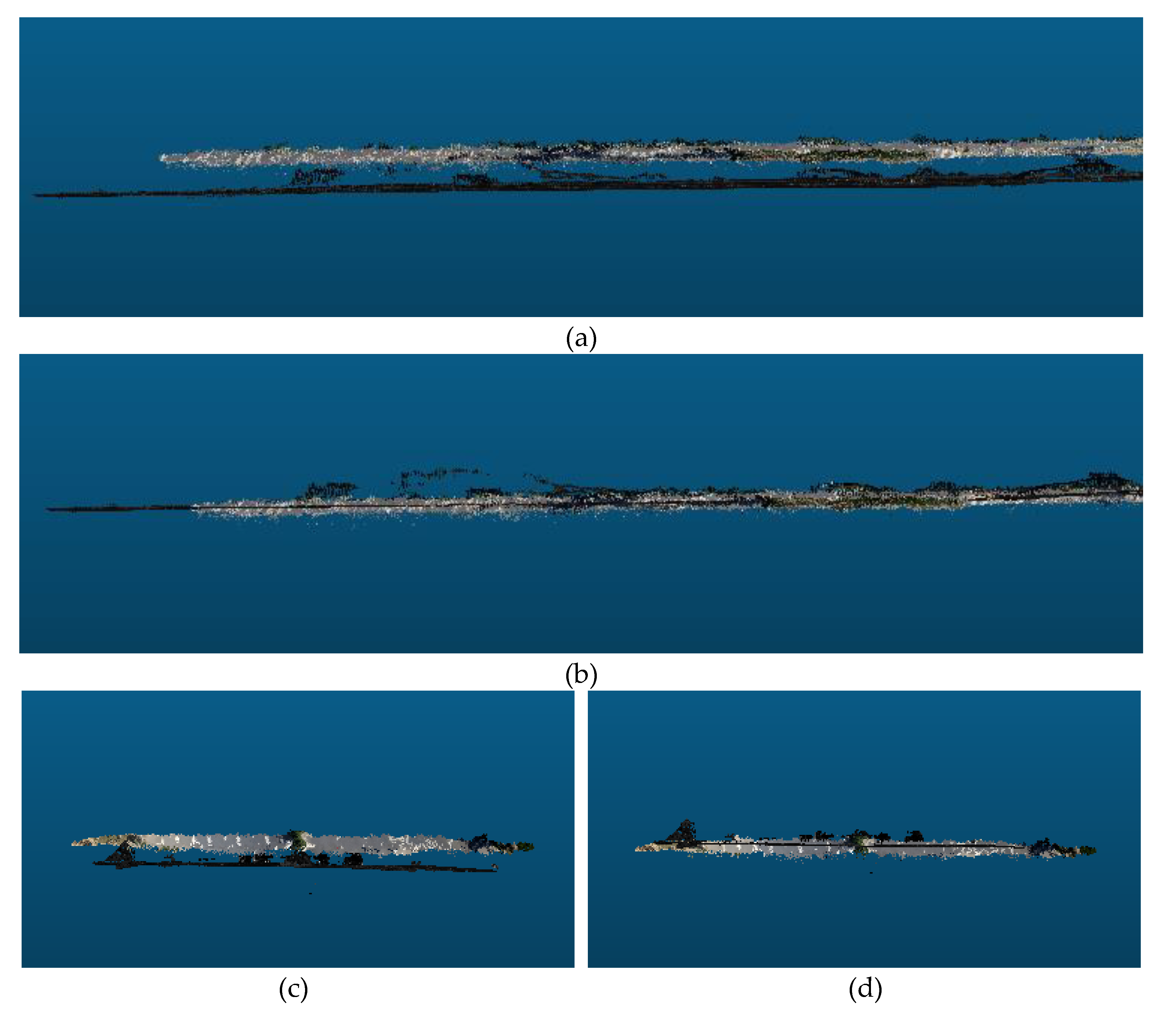
We perform dense matching using the corrected image external orientation elements, and in comparison with the dense point cloud obtained by the original image external orientation elements, we could visually find that the offsets in horizontal direction and in vertical direction are getting smaller in Figure 9, after LiDAR point cloud-assisted aerotriangulation. Note that the black points are vehicle-borne LiDAR points, while the gray-like points are dense points generated from UAV images.
Again, in order to visually verify the accuracy of this method, the vehicle-borne LiDAR point cloud of the road is extracted from the total vehicle-borne LiDAR point cloud, and it is back-projected onto the corresponding images according to the external orientation elements obtained before and after the LiDAR point cloud constraint. The accuracy of aerotriangulation can also be judged by observing the coincidence degree between projection point and image.
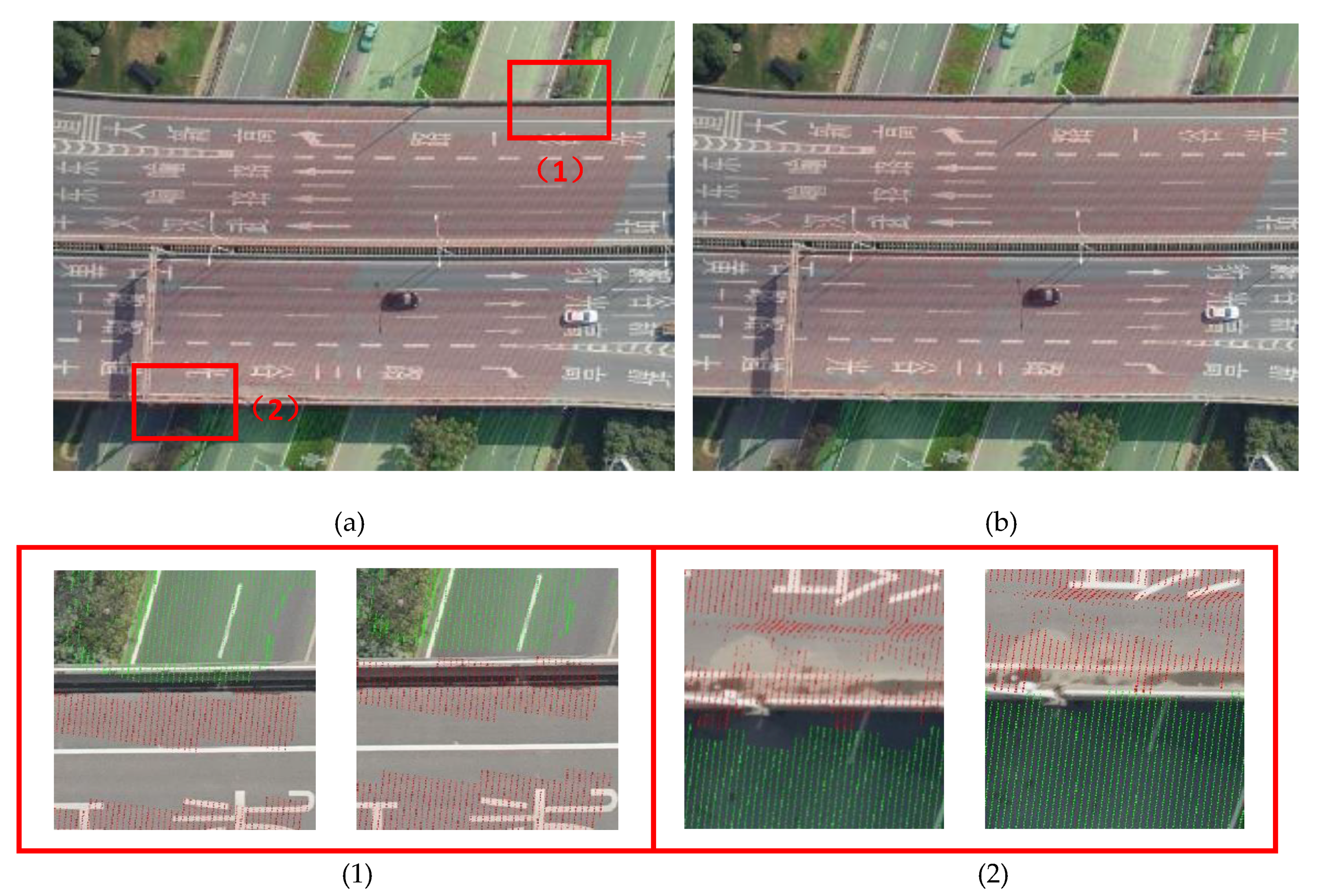
As shown in Figure 10, the vehicle-borne LiDAR point cloud of the overpass is projected onto the corresponding image, and the projection point of the LiDAR point cloud is colored according to the elevation. The overpass points that own the lower elevation (bottom of the bridge, <32 m) are green, and the higher elevation (bridge Upper, ≥32 meters) points are red. From the details of the overpasses (1) and (2) in Figure 10, we can see that before the LiDAR point cloud constrained aerotriangulation there are misalignments at the edges. In other words, part of the bottom of the bridge is back-projected on the bridge, while some of the points on the bridge are back-projected on the bottom of the bridge. However, after being constrained by the LiDAR point cloud, the coincidence accuracy is significantly improved.
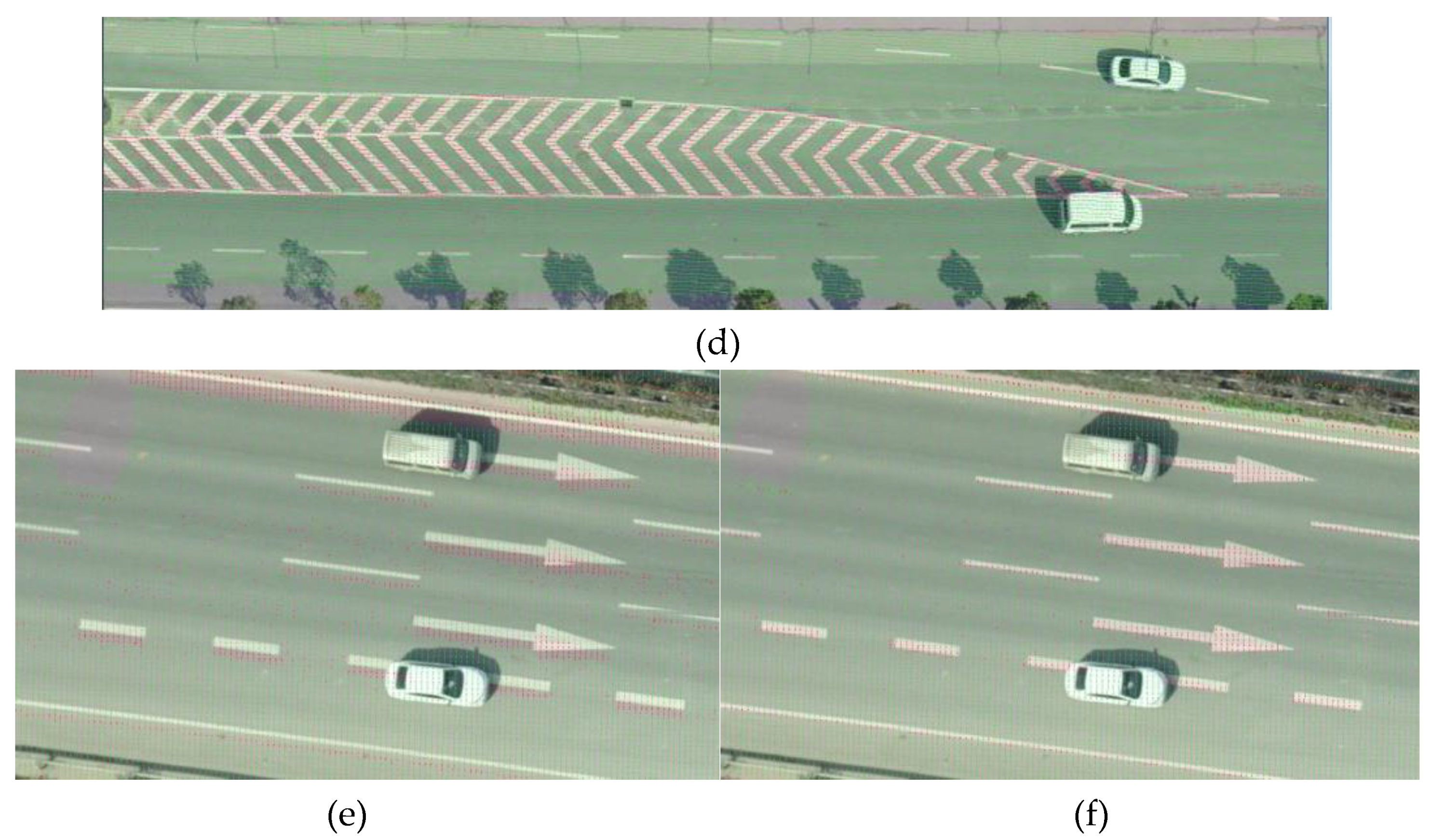
Using the characteristics of obvious contrast between road markings and asphalt pavement, the effectiveness of this method can also be verified by the deviation of road markings. In the LiDAR point cloud, three kinds of common road markings, i.e., “entry entrance line”, “diverging line”, and “indicating arrow” are selected and back projected, and the projected points are colored according to LiDAR point cloud intensity. The contrast between the projection results before and after the LiDAR point cloud constraint is shown in Figure 11. Before the LiDAR point cloud constraint, the projected points of the road markings are significantly shifted. After the LiDAR point cloud constraint, the projection point offset is very small, with an offset of about 3-5 pixels. The coincidence accuracy is significantly improved.

5. Conclusions

To address the problem of low accuracy of aerotriangulation under sparse control, this paper proposes a non-rigid method of LiDAR point cloud-assisted aerotriangulation. The method does not require complicated feature extraction and matching between the images and the point cloud, and can handle the non-rigid distortion problem of the images. Through experiments and accuracy evaluation, the results show that the RMSE of the checkpoints on the x, y, and z axes are 0.113 m, 0.158 m, and 0.082 m after being constrained by the LiDAR point cloud. The effectiveness and robustness of the proposed method are verified. Since the number of control points has a great correlation with the terrain and characteristics of experimental data, we will explore adding other feature constraints on the basis of this research to achieve uncontrolled aerotriangulation.

Author Contributions

Conceptualization, Z.J.; methodology, L.Z.; software, Y.L. and M.S.; data curation, Q.S.; writing—original draft preparation, L.Z. and Y.L.; writing—review and editing, M.Y.; visualization, M.S.; supervision, Z.J. and L.Z.; funding acquisition, Z.J.

Funding

This work is supported by The National Key Research and Development Program of China (2018YFB0505003) and Shanghai automotive industry technology development fund of China (1818).

Acknowledgments

The authors thank the anonymous reviewers and members of the editorial team for the comments and contributions. The authors would like to thank Anhui Huadian Engineering Consultating & Design CO., LTD for providing the UAV data.

Conflicts of Interest

The authors declare no conflict of interest. The funders had no role in the design of the study; in the collection, analyses, or interpretation of data; in the writing of the manuscript, or in the decision to publish the results

References

  1. Honkavaara, E.; Saari, H.; Kaivosoja, J.; Pölönen, I.; Hakala, T.; Litkey, P.; Mäkynen, J.; Pesonen, L. Processing and Assessment of Spectrometric, Stereoscopic Imagery Collected Using a Lightweight UAV Spectral Camera for Precision Agriculture. Remote Sens. 2013, 5, 5006. [Google Scholar] [CrossRef]
  2. Jaud, M.; Passot, S.; Le Bivic, R.; Delacourt, C.; Grandjean, P.; Le Dantec, N. Assessing the Accuracy of High Resolution Digital Surface Models Computed by PhotoScan® and MicMac® in Sub-Optimal Survey Conditions. Remote Sens. 2016, 8, 465. [Google Scholar] [CrossRef]
  3. Phantom 4 RTK Sheet. Available online: https://www.dji.com/cn/phantom-4-rtk/info (accessed on 14 June 2018).
  4. Cui, T.; Ji, S.; Shan, J.; Gong, J.; Liu, K. Line-Based Registration of Panoramic Images and LiDAR Point Clouds for Mobile Mapping. Sensors 2017, 17, 70. [Google Scholar] [CrossRef] [PubMed]
  5. Hirschmuller, H. Stereo processing by semiglobal matching and mutual information. IEEE Trans. Pattern Anal. Mach. Intell. 2008, 30, 328–341. [Google Scholar] [CrossRef]
  6. Bodensteiner, C.; Arens, M. Real-time 2D video/3D LiDAR registration. In Proceedings of the IEEE 21st International Conference on Pattern Recognition, Tsukuba, Japan, 11–15 November 2012; pp. 2206–2209. [Google Scholar]
  7. Furukawa, Y.; Ponce, J. Accurate, dense, and robust multiview stereopsis. IEEE Trans. Pattern Anal. Mach. Intell. 2010, 32, 1362–1376. [Google Scholar] [CrossRef]
  8. Lee, J.; Cai, X.; Schonlieb, C.-B.; Coomes, D.A. Nonparametric Image Registration of Airborne LiDAR, Hyperspectral and Photographic Imagery of Wooded Landscapes. IEEE Trans. Geosci. Remote Sens. 2015, 53, 6073–6084. [Google Scholar] [CrossRef]
  9. Vu, H.H.; Labatut, P.; Pons, J.P.; Keriven, R. High accuracy and visibility-consistent dense multiview stereo. IEEE Trans. Pattern Anal. Mach. Intell. 2012, 34, 889–901. [Google Scholar] [CrossRef] [PubMed]
  10. ContextCapture—3D Reality Modeling Software. Available online: https://www.bentley.com/en/ products/brands/contextcapture (accessed on 12 September 2018).
  11. Lowe, D.G. Distinctive Image Features from Scale-Invariant Keypoints. Int. J. Comput. Vis. 2004, 60, 91–110. [Google Scholar] [CrossRef] [Green Version]
  12. Li, N.; Huang, X.; Zhang, F.; Wang, L. Registration of Aerial Imagery and Lidar Data in Desert Areas Using the Centroids of Bushes as Control Information. Photogramm. Eng. Remote Sens. 2013, 79, 743–752. [Google Scholar] [CrossRef]
  13. Habib, A.F.; Shin, S.; Kim, C.; Al-Durgham, M. Integration of Photogrammetric and LIDAR Data in a Multi-Primitive Triangulation Environment. In Innovations in 3D Geo Information Systems; Springer: Berlin, Germany, 2006; pp. 29–45. [Google Scholar]
  14. Habib, A.; Ghanma, M.; Morgan, M.; Al-Ruzouq, R. Photogrammetric and Lidar Data Registration Using Linear Features. Photogramm. Eng. Remote Sens. 2005, 71, 699–707. [Google Scholar] [CrossRef]
  15. Zhang, Y.; Xiong, X.; Shen, X. Automatic registration of urban aerial imagery with airborne LiDAR data. Int. J. Remote Sens. 2012, 16, 579–595. [Google Scholar]
  16. Sheng, Q.; Wang, Q.; Zhang, X.; Wang, B.; Zhang, B.; Zhang, Z. Registration of Urban Aerial Image and LiDAR Based on Line Vectors. Appl. Sci. 2017, 7, 965. [Google Scholar] [CrossRef]
  17. Yang, B.; Chen, C. Automatic registration of UAV-borne sequent images and LiDAR data. ISPRS J. Photogramm. Remote Sens. 2015, 101, 262–274. [Google Scholar] [CrossRef]
  18. Hartley, R.; Zisserman, A. Multiple View Geometry in Computer Vision; Cambridge University Press: Cambridge, UK, 2000; pp. 1865–1872. [Google Scholar]
  19. Schönberger, J.L.; Frahm, J.M. Structure-from-Motion Revisited. In Proceedings of the 2016 IEEE Conference on Computer Vision and Pattern Recognition (CVPR), Las Vegas, NV, USA, 26 June–1 July 2016; pp. 4104–4113. [Google Scholar]
  20. Mikhail, E.; Bethel, J.; McGlone, J.C. Introduction to Modern Photogrammetry; Wiley: New York, NY, USA, 2001; p. 496. [Google Scholar]
  21. Abayowa, B.O.; Yilmaz, A.; Hardie, R.C. Automatic registration of optical aerial imagery to a LiDAR point cloud for generation of city models. ISPRS J. Photogramm. Remote Sens. 2015, 106, 68–81. [Google Scholar] [CrossRef]
  22. Besl, P.J.; McKay, N.D. A method for registration of 3-D shapes. IEEE Trans. Pattern Anal. Mach. Intell. 1992, 14, 239–256. [Google Scholar] [CrossRef]
  23. Chi, C.; Yang, B.; Peng, X. Automatic Registration of Low Altitude UAV Sequent Images and Laser Point Clouds. Acta Geod. Cartogr. Sin. 2015, 44, 518–525. [Google Scholar]
  24. Li, Y.; Low, K.-L. Automatic registration of color images to 3D geometry. In Proceedings of the 2009 Computer Graphics International Conference, Victoria, BC, Canada; 2016; pp. 21–28. [Google Scholar]
  25. Zheng, S.; Huang, R.; Zhou, Y. Registration of optical images with lidar data and its accuracy assessment. Photogramm. Eng. Remote Sens. 2013, 79, 731–741. [Google Scholar] [CrossRef]
  26. Swart, A.; Broere, J.; Veltkamp, R.; Tan, R. Refined Non-rigid Registration of a Panoramic Image Sequence to a LiDAR Point Cloud. Photogramm. Image Anal. Lect. Notes Comput. Sci. 2010, 6952, 73–84. [Google Scholar]
  27. Ila, V.; Polok, L.; Solony, M.; Istenic, K. Fast Incremental Bundle Adjustment with Covariance Recovery. In Proceedings of the 2017 International Conference on 3D Vision (3DV), Qingdao, China, 10–12 October 2017; pp. 175–184. [Google Scholar]
  28. Triggs, B.; McLauchlan, P.F.; Hartley, R.I.; Fitzgibbon, A.W. Bundle Adjustment—A Modern Synthesis. In Vision Algorithms: Theory and Practice; Springer: Berlin, Germany, 2000; pp. 298–372. [Google Scholar]
  29. Chen, Y.; Medioni, G. Object modelling by registration of multiple range images. Image Vis. Comput. 1992, 10, 145–155. [Google Scholar] [CrossRef]
  30. Arya, S.; Mount, D.M.; Netanyahu, N.S.; Silverman, R.; Wu, A.Y. An optimal algorithm for approximate nearest neighbor searching fixed dimensions. J. ACM 1998, 45, 891–923. [Google Scholar] [CrossRef] [Green Version]
  31. Bentley, J.L. Multidimensional binary search trees used for associative searching. Commun. ACM 1975, 18, 509–517. [Google Scholar] [CrossRef]
  32. K-d_tree. Available online: https://en.wikipedia.org/wiki/K-d_tree (accessed on 12 September 2018).
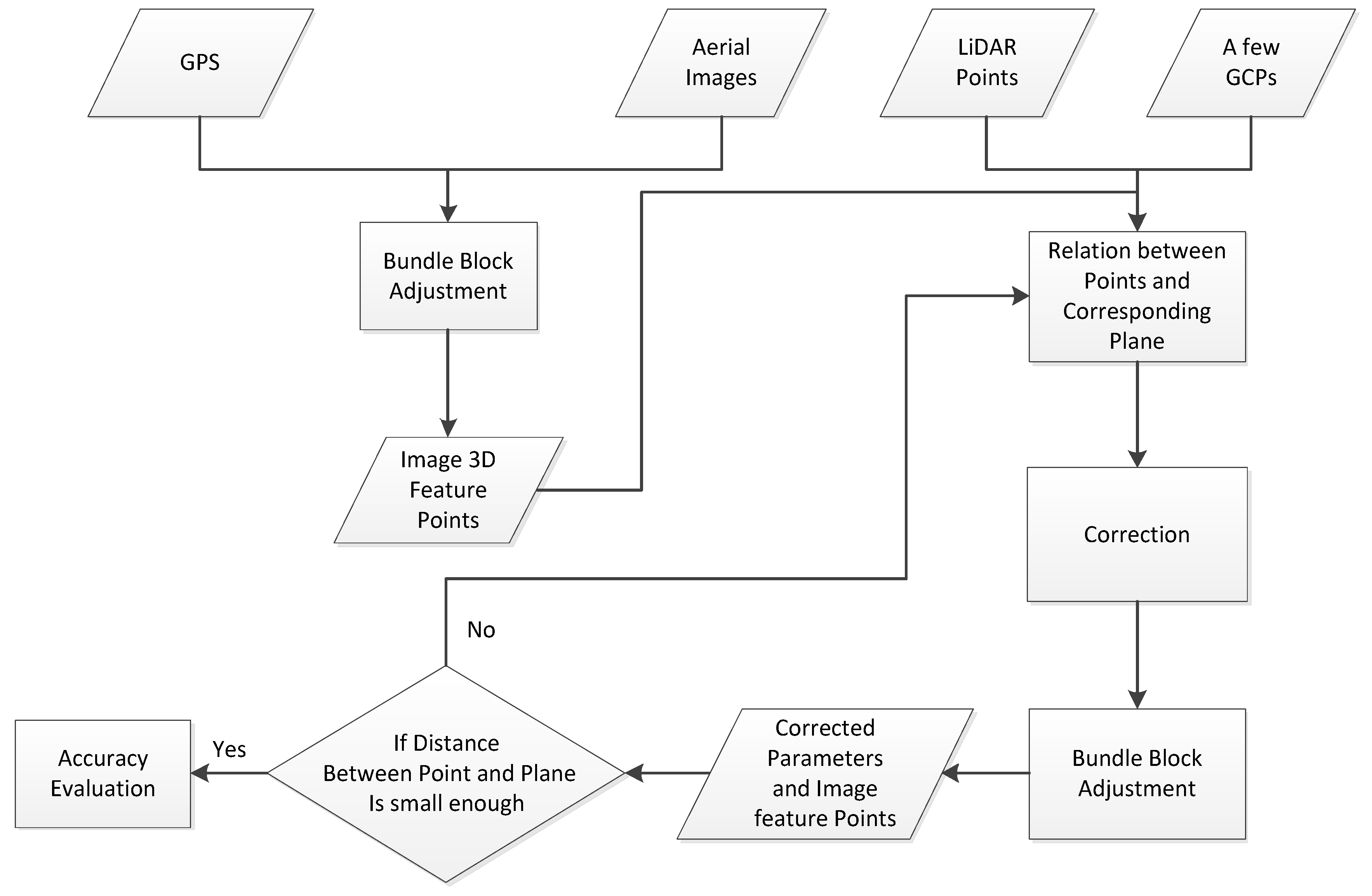
Figure 1. Flow chart of light detection and ranging (LiDAR) point cloud-assisted aerotriangulation.
Remotesensing 11 01188 g001
Figure 2. The definition of coordinate system.
Remotesensing 11 01188 g002
Figure 3. The geolocation between LiDAR and images.
Remotesensing 11 01188 g003
Figure 4. Different situations of three-dimentional (3D) feature points.
Remotesensing 11 01188 g004
Figure 5. Camera location and image overlap degree.
Remotesensing 11 01188 g005
Figure 6. Detail of study area: (a) Orthophoto image; (b) vehicle-borne LiDAR Data.
Remotesensing 11 01188 g006
Figure 7. Overlap diagram of LiDAR and 3D feature point.
Remotesensing 11 01188 g007
Figure 8. RMSE of checkpoint during adjustment iteration.
Remotesensing 11 01188 g008
Figure 9. Vehicle-borne LiDAR and image-dense point cloud: (a) Longitudinal section before LiDAR constrain; (b) longitudinal section after LiDAR constrain; (c) transverse section before LiDAR constrain; (d) transverse section after LiDAR constrain.
Remotesensing 11 01188 g009
Figure 10. Overpass point back projection: (a) Before LiDAR constrain; (b) After LiDAR constrain
Remotesensing 11 01188 g010
Figure 11. Land mark back projection: (a,b) Entry entrance line before and after LiDAR constrain; (c,d) diverging line before and after LiDAR constrain; (e,f) indicating arrow before and after LiDAR constrain.
Remotesensing 11 01188 g011aRemotesensing 11 01188 g011b
Table 1. Detail information of UAV images.
DataSensorImage Size (Pixels)Focal Length (mm)Cell Size (mm)Resolution
(m)
ImagesSONY ILCE-7R7360*491235.80.00480.04
Table 2. Detail information of vehicle-borne LiDAR.
DataSensorsDistance between Point Cloud (m)The Number of Point Cloud
LiDAR pointLeica ALS50-II0.130.5billion
Table 3. The RMSE of checkpoints before and after LiDAR point cloud constrain (m).
CheckpointBefore LiDAR ConstrainAfter LiDAR Constrain
d x d y d z d x d y d z
10.237-0.2141.7650.201-0.181-0.170
20.073-0.1251.998-0.058-0.118-0.007
30.017-0.0221.670-0.001-0.010-0.053
4-0.184-0.235-1.090-0.099-0.238-0.059
5-0.063-0.0460.861-0.062-0.0390.072
6-0.0360.1270.230-0.0410.1310.008
7-0.075-0.2470.103-0.079-0.243-0.100
80.090-0.2820.8040.074-0.252-0.022
90.0770.3220.9830.056-0.1400.030
100.159-0.3551.0370.133-0.293-0.005
110.159-0.0501.7360.122-0.014-0.123
12-0.095-0.2201.788-0.132-0.190-0.088
130.304-0.0331.8080.267-0.009-0.059
140.016-0.0761.768-0.021-0.051-0.042
150.134-0.2041.7460.099-0.182-0.054
160.1560.1570.5560.1410.163-0.038
170.1200.0280.2080.1090.043-0.189
Maximum error0.3040.3551.9980.2670.2930.189
Minimum
error
0.0160.0220.1030.0010.0090.005
The mean
error
0.1400.1931.3410.1180.1630.084