Article

Comparing Remotely-Sensed Surface Energy Balance Evapotranspiration Estimates in Heterogeneous and Data-Limited Regions: A Case Study of Tanzania’s Kilombero Valley

1
Department of Physical Geography, Stockholm University, SE 106 91 Stockholm, Sweden
2
Department of Water Resources Engineering (WRE), University of Dar es Salaam, P.O. Box 35131 Dar es Salaam, Tanzania
3
Water Institute, P.O. Box 35059 Dar es Salaam, Tanzania
4
The Nature Conservancy, 2350 NJ-47, Delmont, NJ 08314, USA
*
Author to whom correspondence should be addressed.
Remote Sens. 2019, 11(11), 1289; https://doi.org/10.3390/rs11111289
Submission received: 5 April 2019 / Revised: 18 May 2019 / Accepted: 27 May 2019 / Published: 30 May 2019

Abstract

:
Evapotranspiration (ET) plays a crucial role in integrated water resources planning, development and management, especially in tropical and arid regions. Determining ET is not straightforward due to the heterogeneity and complexity found in real-world hydrological basins. This situation is often compounded in regions with limited hydro-meteorological data that are facing rapid development of irrigated agriculture. Remote sensing (RS) techniques have proven useful in this regard. In this study, we compared the daily actual ET estimates derived from 3 remotely-sensed surface energy balance (SEB) models, namely, the Surface Energy Balance Algorithm for Land (SEBAL) model, the Operational Simplified Surface Energy Balance (SSEBop) model, and the Simplified Surface Balance Index (S-SEBI) model. These products were generated using the Moderate Resolution Imaging Spectroradiometer (MODIS) satellite imagery for a total of 44 satellite overpasses in 2005, 2010, and 2015 in the heterogeneous, highly-utilized, rapidly-developing and data-limited Kilombero Valley (KV) river basin in Tanzania, eastern Africa. Our results revealed that the SEBAL model had a relatively high ET compared to other models and the SSEBop model had relatively low ET compared to the other models. In addition, we found that the S-SEBI model had a statistically similar ET as the ensemble mean of all models. Further comparison of SEB models’ ET estimates across different land cover classes and different spatial scales revealed that almost all models’ ET estimates were statistically comparable (based on the Wilcoxon’s test and the Levene’s test at a 95% confidence level), which implies fidelity between and reliability of the ET estimates. Moreover, all SEB models managed to capture the two spatially-distinct ET regimes in KV: the stable/permanent ET regime on the mountainous parts of the KV and the seasonally varied ET over the floodplain which contains a Ramsar site (Kilombero Valley Floodplain). Our results have the potential to be used in hydrological modelling to explore and develop integrated water resources management in the valley. We believe that our approach can be applied elsewhere in the world especially where observed meteorological variables are limited.

Graphical Abstract

1. Introduction

Evapotranspiration (ET) is the term used to represent the combined flux from two different pathways of water vaporization in environmental systems, namely, abiotic water evaporation from open water bodies (e.g., ocean, lakes, and swamps), soil pores, and surfaces of leaves (cuticle), and biotic leaf transpiration due to diffusion of water molecules from leaf chloroplasts to the atmosphere through stomata [1]. ET is a key component of the hydrological cycle [2] and an important part of the energy and water balance in agricultural ecosystems [3]. For example, land surface ET accounts for approximately 60% of the mean annual land precipitation in the global hydrological cycle [2]. Studies of ET in irrigated agricultural areas have reported the mean annual (actual) ET to accounts for more than 60% of the mean annual precipitation [4,5].
Accurate information on the spatial and temporal variability of ET can be useful in water resource management. For example, it can help to improve water use efficiency for agricultural crops, better allocate water resources in a river basin, constrain the hydrological model, provide boundary conditions for numerical weather forecasting, and detect forest health and its vulnerability to fire [6,7]. However, getting accurate information on ET is not a straightforward process due to the natural heterogeneity and complexity of ET and other hydrological processes. ET is characterized by complex spatiotemporal changes due to the wide spatial variability of precipitation (in terms of frequency and/or intensity), vegetation types and densities, and hydraulic characteristics of soils, and the wide temporal variability of climate [8]. Human-induced climate change and intensified human activities make ET estimation even more complex [9,10]. Traditional methods (in-situ measurements) used to estimate ET include: weighing Lysimeters, Eddy Covariance (EC) systems, evaporation pans, and Bowen ratio techniques. All these methods provide point estimates which are mainly applicable (reliable/representative) at a field/local scale [11,12,13], and their application beyond this scale (such as the river basin scale) requires a good number of measurements (e.g., many weighing lysimeters). Obtaining several measurements is in most cases prohibitively expensive, especially in developing countries typically found in the so-called Global South. These traditional ET estimation methods become (practically) inapplicable when resource management scales get large (such as regional or basin-wide scales), mainly due to the heterogeneity of the land surfaces, and the complex nature of heat transfer processes governing the ET [14].
Development of remote sensing (RS) techniques has now enabled researchers to implement various ET estimation algorithms as an alternative approach for estimating ET over large areas (from the river basin scale up to the global scale) where the applicability of traditional methods could be limited [15]. Typical RS-based ET estimation algorithms include the Surface Energy Balance Algorithm for Land (SEBAL) model [16], Operational Simplified Surface Energy Balance (SSEBop) model [17], Surface Energy Balance System (SEBS) model [14], Mapping Evapotranspiration at a high-Resolution with Internalized Calibration (METRIC) model [18], and Simplified Surface Energy Balance Index (S-SEBI) model [19]. These RS-based ET estimation algorithms utilize land surface characteristics derived from the remotely sensed multi-spectral data from visible to thermal infrared bands of the electromagnetic spectrum to estimate ET [15]. Different remote sensing sensors onboard different satellites/platforms have the capability of providing these multi-spectral data in various temporal and spatial resolutions. These satellite platforms include Landsat, Advanced Spaceborne Thermal Emission and Reflection Radiometer (ASTER), Advanced Very High-Resolution Radiometer (AVHRR), Visible Infrared Imaging Radiometer Suite (VIIRS), and the Moderate Resolution Imaging Spectroradiometer (MODIS).
One of the major advantages of the RS-based ET estimation algorithms is their capability of estimating ET without quantifying other complex hydrological processes [7]. Review studies on the accuracy of ET estimated by these algorithms have reported accuracies that vary from 67% to 97% for daily ET estimates, and rise above 94% for seasonal ET estimates [20,21]. These accuracies were achieved by comparing the ET derived from the RS-based ET estimation algorithms against ET derived from the traditional methods of estimating ET (e.g., weighing lysimeters, and eddy covariance (EC) systems). An overview of the advantages, limitations, and uncertainties of the widely used RS-based ET estimation algorithms can be found in Li et al. [15].
Each approach has certain benefits and potential limitations. The Surface Energy Balance Algorithm for Land (SEBAL), for example, is a physically based thermal infrared RS-based ET estimation model developed by Bastiaanssen et al. [16], mainly, for the purpose of estimating the actual ET (AET) for the cloud-free (clear-sky) days across different ecosystems. The cloud-free day is a requirement of any thermal infrared RS-based ET estimation algorithm [21]. The main advantages of the SEBAL model are the following: it requires minimum ground measurements (mainly wind speed), it has automatic internal calibration via Monin-Obukhov schemes [22], and it does not need accurate atmospheric corrections [15,23].
There are still open questions around the robustness of any of these RS-based models and which can be considered the “best” or at least useful in more applied settings. This question comes to the forefront in regions where large seasonal variations exist; where there are limited data for estimating ET using traditional approaches; and where water resources are rapidly developing in connection to population growth and agricultural intensification. For example, the Kilombero Valley (KV) river basin located in the south-central part of Tanzania, in East Africa (Figure 1) is currently facing rapid development of dry land irrigated agriculture following the implementation of the Southern Agricultural Growth Corridor of Tanzania (SAGCOT) initiative. SAGCOT is an inclusive, multi-stakeholder partnership launched in 2010 with the aim of improving agricultural productivity, food security, and livelihoods in Tanzania through small-scale and large-scale irrigation schemes [24]. Water abstractions from the river system for irrigation and changing the landscape water use patterns through the conversion of other land use/covers into agriculture not only affect water availability and quality [25] in the KV basin, but also has an impact on the proposed Stiegler’s Gorge dam. The dam is targeted for hydroelectric power generation (2100 megawatts) downstream of the basin. Therefore, an accurate estimation of the actual ET is certainly crucial for the sustainability of integrated water resources management (IWRM) in the KV basin, the sustainability of the Ramsar site (Kilombero Valley Floodplain) located in the vicinity of the floodplain in the KV basin (Figure 1), and the operation of the proposed Stiegler’s Gorge hydroelectric power generation. Unfortunately (or perhaps problematically), the basin has poor coverage of the hydro-meteorological network [24,26,27,28] layering additional challenges on those faced to achieve sustainable development in SAGCOT. Understanding the basic patterns of ET and how these vary seasonally and interannually—and in response to coupled land-water use changes—would be a huge step towards the sustainable development and management of KV’s water resources.
To address the need for understanding, this study compared the actual ET estimates computed using 3 surface energy balance (SEB) models, namely, the SEBAL model [16], the SSEBop model [17], and the S-SEBI model [19] in the heterogeneous, data-scarce, and highly utilized KV river basin using 250 m, 8-day MODIS land products for the three distinct years of 2005 (five years before SAGCOT), 2010 (beginning of the SAGCOT), and 2015 (five years after SAGCOT). We hypothesized that contrasting ET estimates obtained from 3 distinct years (each with a different degree of land management practices) for model comparison provides more insight on similarities (congruence) and differences among models than using consecutive years where the trend of changes in land management practices is more less gradual (or zero). Our motivation is an attempt to leverage RS-based ET estimation techniques in a heterogeneous, data-limited, and highly utilized setting to improve the understanding of ET spatial variations.

2. Materials and Methods

This section briefly covers the description of the study area (Kilombero Valley (KV) river basin), together with the sources of/and different types of the Moderate Resolution Imaging Spectroradiometer (MODIS) datasets and other ancillary datasets used in this study. Lastly, the brief descriptions and applications of the Surface Energy Balance Algorithm for the Land (SEBAL) model [16], the Operational Simplified Surface Energy Balance (SSEBop) model [17], and the Simplified Surface Energy Balance Index (S-SEBI) model [19] will be given together with the approach used to compare models in this study.

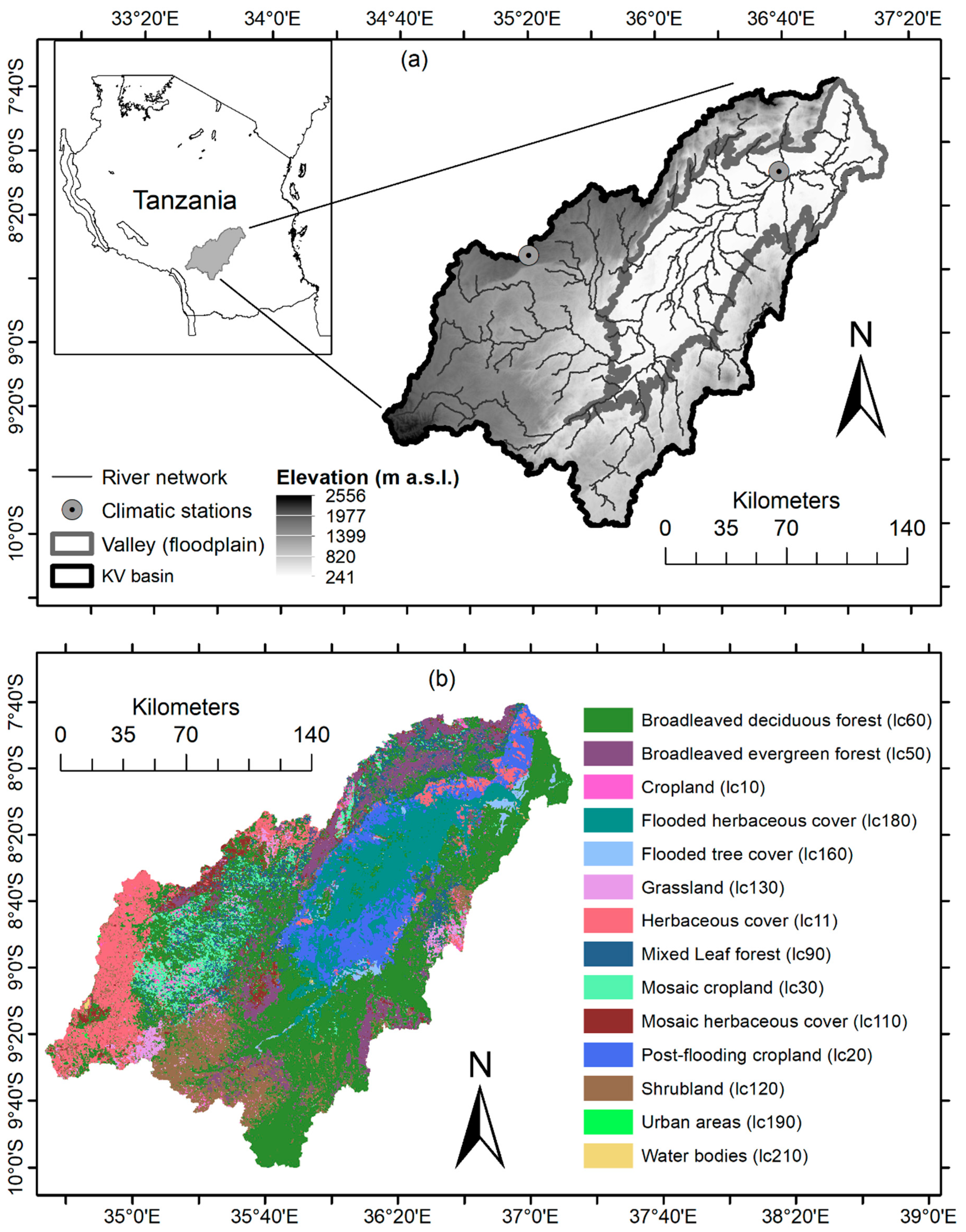
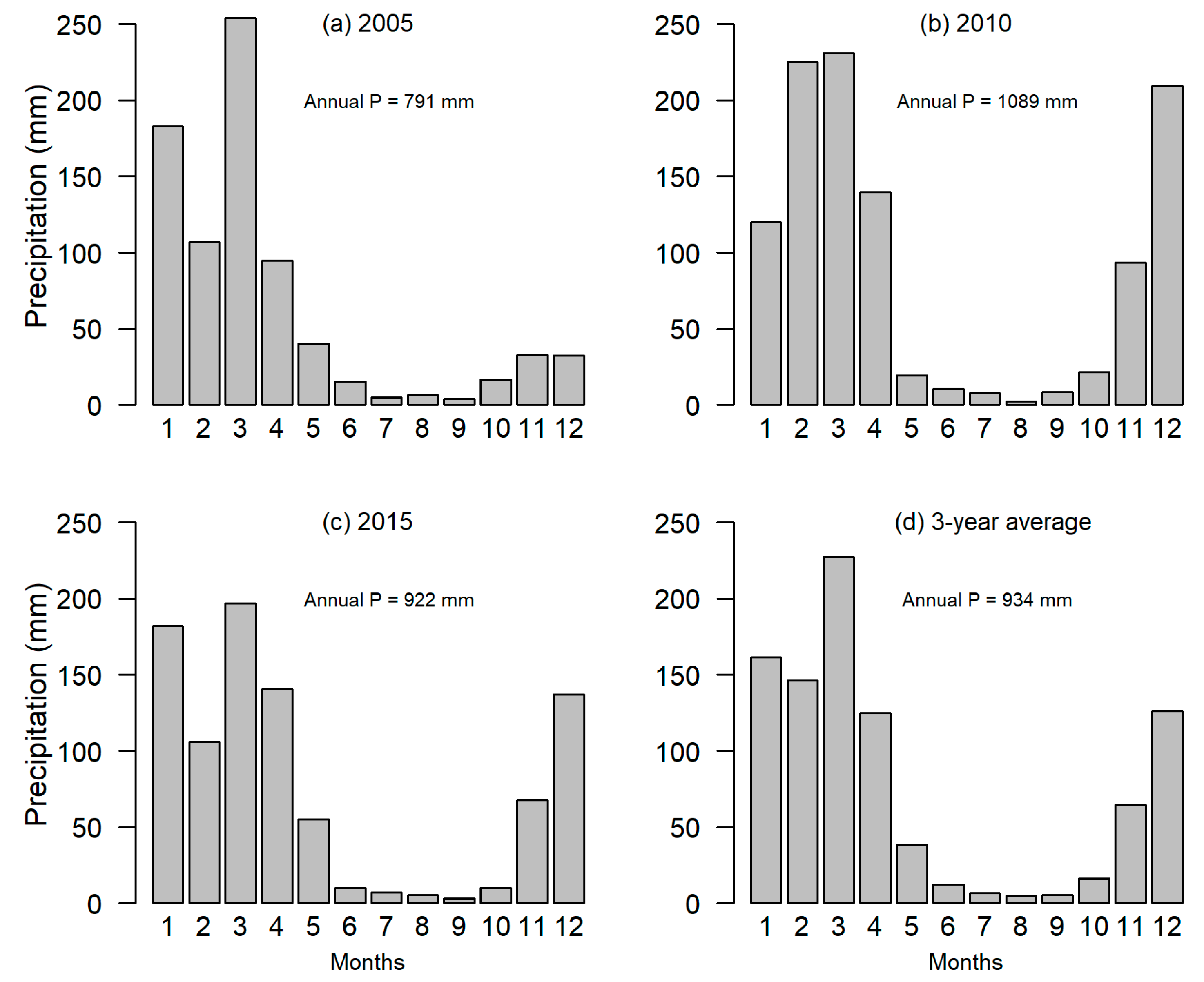
2.1. Kilombero Valley (KV) River Basin: Site Description and Ancillary Datasets

This study was undertaken in the Kilombero Valley (KV) river basin (Figure 1) located in the southern central part of Tanzanian country in East Africa. The Valley is situated between 34°33′ and 37°20′ east of the Greenwich meridian (i.e., Longitudes) and between 7°39′ and 10°01′ south of the equator (i.e., Latitudes). The KV covers an approximate area of 34,000 km2 (up to Swero river gauging station) and forms one of the four principal sub-basins of the Rufiji River Basin (RRB). Udzungwa Mountains (2576 m high) border the KV river basin in the north-western part, and Mbarika Mountains (1516 m high) and Mahenge escarpment form the south-eastern border of the basin [29]. These mountains (Udzungwa and Mbarika) form the headwaters of the KV river system through their dense network of tributaries. The main river, namely, the Kilombero river, becomes a braided river when it gets to the central part of the valley. The whole valley is characterized by a complex system of perennial and seasonal river networks, with several numbers of ponds, oxbow lakes, swamps, and wetlands [30]. The Kilombero Valley Floodplain has an approximate surface area of 7,967 km2 and was designated as a Ramsar site (i.e., the wetland of international environmental importance) in 2002 (http://www.ramsar.org).
The KV river basin experiences a sub-tropical climate with the mean annual precipitation (during the period 1998–2010) ranging from 1200 mm to 1400 mm in the valley bottom, and from 1500 mm to 2100 mm in the mountainous parts of the KV basin [26]. More than 55% of the total mean annual precipitation goes back to the atmosphere as Evapotranspiration [28,31]. The mean daily temperature is around 24 °C in the valley bottom and decreases to around 17 °C in the mountainous parts of the basin. The KV basin is part of the East African Rift Valley formed by Pliocene faulting. While the highlands parts of the basin are rich of crystalline limestone, schists, graphite, and gneisses, the lower parts are underlain by Karoo sediments (sandstones, conglomerates and shales), and the valley bottom is characterized by alluvial fans and Miombo plains [32]. Climate, geology and geomorphology are the main controllers of groundwater recharge which mainly originates from the rainwater infiltration from the high altitudes. The basin has an average aquifer transmissivity of 0.18 m2/min [33] and the mean annual flow of 13.8 billion cubic meters [34]. Recent studies by Koutsouris and Lyon [27] and Burghof et al. [35] have revealed the significant contribution of groundwater discharge to the seasonal streamflow variability in the KV basin.
A total of 5 climatic stations from Rufiji Basin Water Office (RBWO) were used in this study (Figure 1) to provide time series of air temperature (Maximum and Minimum), wind speed, and relative humidity (Table 1). All time series were screened for potential inaccuracies and all suspicious data (less than 2%) were removed and replaced by their corresponding long-term averages (2005–2015). The Inverse Distance Weighting (IDW) interpolation method was used to interpolate these climatic data (a lapse of 6.5 °C/km was used when interpolating the time series of air temperature) to cover the entire spatial extent of the KV basin. Climatic stations are not spatially distributed over the KV basin; therefore, the interpolated time series remains one of the potential sources of uncertainty in the final actual evapotranspiration (ET) estimates. It is noteworthy that neither of the SEB models used in this study utilizes precipitation (P) data, therefore, precipitation data were used only to assess the reliability of the ET estimates because precipitation is one of the key factors that control the spatiotemporal dynamics of ET. Other factors include land cover, soil type, water availability from other sources (such as irrigation), climatic conditions, elevation, and solar radiation [23].
In 2005, KV river basin had a relatively low annual precipitation (P = 791 mm) compared to other years (i.e., 2010 (P = 1089 mm/year) and 2015 (P = 922 mm/year)) (Figure 2). In addition to climatic data, a Shuttle Radar Topography Mission (SRTM) digital elevation model (DEM) with a 90 m raster Resolution was used to delineate the catchment (Figure 1) and to provide other topographic information (such as the slope and aspect). Vegetation coverage and soil information (Table 2) were accessed from the global land cover map for the year 2015 provided by the European Space Agency (ESA) Climate Change Initiative (CCI) project (CCI-LC project) (http://maps.elie.ucl.ac.be/CCI/viewer/download.php, accessed on 11 February 2019) and the Harmonized World Soil Database (HWSD) [36] respectively. Spatial resolutions of these spatial datasets ranged from 1:100000 to 1:300000. This study divided the basin into two parts—the uplands (Mountain-forests) with an elevation greater than about 670 m and the wetland-valley (Floodplain) with elevation equal to or less than about 670 m—based on the topography (Table 2). The uplands have relatively more proportions of forested lands and Acrisol soils. The wetland-valley, on the other hand, has relatively more proportions of herbaceous and Fluvisol soils. Forest and Acrisol are the main vegetation and soil types (respectively) over the entire basin.
The land cover classes for the KV river basin were extracted from the High-Resolution (HR) Land Cover (LC) map (global land cover map) for the year 2015 provided by the European Space Agency (ESA) Climate Change Initiative (CCI) project (CCI-LC project) (http://maps.elie.ucl.ac.be/CCI/viewer/download.php, accessed on 11 February 2019). The CCI-LC project provides consistent annually global land cover maps at 300 m spatial resolution from 1992 to 2015. More details about this project and how these land cover maps were prepared can be accessed through the aforementioned website. For this study, ESA-CCI land cover classes for the KV river basin were reclassified to 14 classes (Figure 1) and used to aggregate the daily ET per land cover class (see subsequent section). Most of the study area was covered by the broadleaved deciduous forest (around 38% of the total area) followed by flooded herbaceous cover (11%) (Table 3). Urban areas and Water bodies each occupied less than 1% of the total study area. It is noteworthy to point out that a large part of the broadleaf deciduous forest is locally known as the ‘Miombo woodland’.

2.2. Overview of Remotely-Sensed Surface Energy Balance Products

Different studies have been undertaken to compare the robustness (in terms of performance) of various RS-based ET estimation models [37,38,39,40]. Interestingly, no specific model has been declared to be the most robust of all because different studies have reported different ranks of best models. Specifically, we find that a particular model can be ranked (in descending order of robustness) first in one study and ranked in other positions in another study which compares almost the same group of models. This inconsistency has been associated with different factors which among others, include climate, the season of the year, and the type of the ecosystem where the study is conducted. In this study, we selected three SEB models, namely, the SEBAL, SSEBop, and S-SEBI models because: they require minimum climatic data, the SEBAL and the SSEBop models have previously been successfully used in Tanzania [4,5] and all of these models (i.e., SEBAL, SSEBop, and S-SEBI models) have been applied and validated across different scales (temporal and spatial) in a wide range of climatological conditions, and ecosystems (e.g., agroecosystems) almost all over the world. For example, the SEBAL model has been applied and validated in different hydrological basins (including data scarce basins in Africa) in more than 30 countries [23]. Some of these hydrological basins and their respective countries include the upper Pangani river basin in Tanzania/Kenya [4], the Gediz basin in Turkey [41], the Sudd, Sobat and Ghazal basins in Sudan [42], the Kingdom of Saudi Arabia (the entire country) [43], the Yakima river basin in the United States of America [23], and the Nansi Lake Wetland in China [44]. We recommend readers to refer to these pieces of literature for more details on the type of data used in the validation process and the accuracies of the validation results. More lists of validation studies can be found in Karimi and Bastiaanssen [21] and Bastiaanssen et al. [23].

2.2.1. MODIS Program

The Moderate Resolution Imaging Spectroradiometer (MODIS) instrument (sensor) has the capability of measuring 36 spectral bands between 0.405 μm and 14.385 μm (i.e., from the visible to thermal-infrared regions of electromagnetic spectrum) at three spatial resolutions: 250 m, 500 m, and 1000 m. It has a viewing swath width of 2330 km and a revisit time of one to two days. It is operated by the National Aeronautics and Space Administration’s (NASA) Earth Observing System (EOS) program. The MODIS instrument operates on two satellites (spacecraft), namely, Terra (launched on 18 December 1999) and Aqua (launched on 04 May 2002). The MODIS instruments on both Terra and Aqua image (view) the same area on the earth at approximately 10:30 AM (on the Terra) and 1:30 PM (on the Aqua) local time. They provide a comprehensive series of global observations of the land, oceans, and the atmosphere. MODIS land (MODLand) products, in particular, are available through the Land Processes Distributed Active Archive Center (LPDAAC) at the U. S. Geological Survey (USGS) Earth Resources Observation and Science (EROS) Data Center (EDC). An overview of MODLand products processing and status is given by Justice at al. [45]. The latest version of MODIS land products is MODIS Version 6 (V006). All MODIS land products used in this manuscript (Table 4) belong to this version (V006). These products were downloaded for free from NASA’s LPDAAC website (https://lpdaac.usgs.gov/).

2.2.2. Preprocessing of MODIS Land Products

The MODIS Land Products required for the SEBAL model include Land Surface Temperature and Emissivity (LST/EMM), Normalized Difference Vegetation Index (NDVI), Leaf Area Index (LAI), and short-wave broadband surface albedo (BRDF-albedo) (Table 4). Preprocessing of MODIS satellite images was done primarily to render them ready (mainly in terms of format, and validity) to be used in the SEBAL model. The whole concept of preprocessing can be grouped into two parts: scaling and resampling of retrieved MODIS images, and correction of invalid pixels in the MODIS images. Invalid pixels in the MODIS images might be due to cloud cover, aerosol content, processing failures, atmospheric disturbances, and/or estimation errors [46]. We used two 16-day NDVI images, namely, MOD13Q1 (from Terra satellite), and MYD13Q1 (from Aqua satellite), which start on day 1 and day 9 of the year respectively, to create 8-day 250 m NDVI images for three years, 2005, 2010 and 2015. This approach is similar to the approach used by Kiptala et al. [4] to generate 8-day 250m NDVI images for subsequent use in the SEBAL model application in Pangani river basin (a transboundary basin between Tanzania and Kenya). We acquired and resampled the other MODIS datasets (Table 4) based on these NDVI images. We scaled all MODIS products using their respective scaling factors to unit conversion the values downloaded directly from the MODIS server (Table 4).
Land Surface Temperature (LST) is the major input variable in all thermal infrared ET estimation algorithms [21] including the SEBAL, SSEBop and S-SEBI models. Therefore, the quality of the LST product is highly important [47]. Therefore, only LST images with valid (good quality) temperature data were selected for at least 90% of pixels covering the study area. This was achieved through analysis of the Quality Assessment Science Data Sets (QA-SDS) which is included in all NASA’s MODIS Land Products. QA-SDS considers the atmospheric conditions in terms of cloud cover, aerosol content, processing failures, algorithm choices, and estimation errors [46,48]. We selected 90% as the minimum threshold for the total number of pixels with valid data to minimize uncertainty especially when filling the missing values (correcting the invalid pixels) to produce continuous satellite data. Different thresholds have been used to select LST images; for example, 95% [10], 80% [49], and 75% [50]. We defined a pixel to have valid data if and only if it has the quality flag of 0 (cloud-free) and/or an accuracy level within ± 1 K. Similar criterion was used by Alemayehu et al. [5] to select images with valid surface temperature data from the MODIS LST images for subsequent use in the ET estimation using the operational simplified surface energy balance (SSEBop) algorithm [17] for the Mara River Basin (Kenya/Tanzania). We assigned all the invalid pixels in the images as the missing values using the R raster package [51] in the R program. We ended up with 18, 14 and 12 sets of good quality images (based on 90% criterion) for the years 2005, 2010, and 2015, respectively (Table 5).
To ensure continuous satellite data, all the missing values in the images were filled using the focal mean of a 3 by 3-pixel window (i.e., the pixel with a missing value is filled by the mean of the 8 pixels’ values surrounding it). The approach of filling the missing values using the descriptive statistics (e.g., mean, maximum, and minimum) of the pixels in the neighborhood has been common in the studies which utilized remotely sensed images [4,5]. We defined this focal mean function (i.e., user-defined function) in the R program and applied it to fill the missing values in the MODIS images using the R raster package [51]. It is noteworthy to point out that we deliberately downloaded (all) the MODIS images for the area which extend beyond the KV river basin (Figure 1) for twofold: first, to ensure that every pixel along the border of the KV river basin is surrounded by six pixels (i.e., to maximize the number of pixels with valid data in the 3 by 3 pixel window in case a pixel with a missing value is located along the border), and second, to maximize the possibility of having representative hot and cold pixels (‘anchor pixels’) which are a necessary condition required by the SEBAL model [16] application. Interestingly, even with this design, there were no valid pixels available within a 3 by 3-pixel window in some of the images. Therefore, we used a temporal interpolation technique proposed by Weiss et al. [52] to fill those missing values. The temporal interpolation has been used in several studies to fill the missing values in remotely sensed images [53,54,55].
The average surface emissivity was computed as the average of Em_31 (from band 31) and Em_32 (from band 32) of the MOD11A2 for the day of the year which has an NDVI image from Terra (i.e., MOD13Q1), and as the average of Em_31 (from band 31) and Em_32 (from band 32) of the MYD11A2 for the day of the year which has an NDVI image from Aqua (i.e., MYD13Q1). This approach of considering surface emissivity as the average of Em_31 (from band 31) and Em_32 (from band 32) has been used in several SEBAL model applications which utilized MODIS images as input datasets (e.g., in Mahmoud and Alazba [43] and Kiptala et al. [4]). It is worth noting that the ‘effective’ emissivity can be greater than 1.0, depending on the vertical temperature and moisture structure near the surface.

2.3. The Surface Energy Balance Algorithm for Land model

The Surface Energy Balance Algorithm for the Land (SEBAL) model [16] is a satellite-based image-processing model which estimates the (instantaneous) actual evapotranspiration (ET) for every individual pixel (cell) of the remote sensing image in terms of the instantaneous latent heat flux ( L E ). The later ( L E ) is computed for every individual pixel (i.e., on a pixel-by-pixel basis) of the remote sensing image as a residual of the surface energy balance/budget (SEB) equation (Equation (1)) at the moment of the satellite overpass. Therefore, in general terms, the SEBAL model can be considered as the model which estimates spatially explicit actual evapotranspiration based on the surface energy balance and satellite remote sensing techniques [44]. The model computes a complete surface radiation balance (Equation (2)) and surface energy balance (Equation (1)) along with the resistances for momentum, heat and water vapor transport for every individual pixel of the remote sensing image [56].
L E = R n G H
where: L E is the latent heat flux (W/m2), R n is the net radiant flux at the surface (W/m2), G is the soil heat flux (W/m2), and H is the sensible heat flux to the air (W/m2).
The SEBAL model computes each of the components of Equation (1) using land surface characteristics such as surface temperature ( T s ), normalized vegetation index ( N D V I ), leaf area index ( L A I ), surface albedo ( α ), and emissivity ( ε ). These land surface characteristics are derived from satellite radiances in the visible, near infrared, and thermal infrared part of the electromagnetic spectrum (EM). It is noteworthy to point out that, different types of satellites such as the Moderate Resolution Imaging Spectroradiometer (MODIS), Advanced Spaceborne Thermal Emission and Reflection Radiometer (ASTER), Advanced Very High-Resolution Radiometer (AVHRR), and Landsat have been used to derive the land surface characteristics needed by the SEBAL model [57,58,59,60]. Additionally, it is important to comment that, during the course of computation of H (Equation (1)), SEBAL model computes resistances for momentum, heat and water vapor transport as a function of wind speed and air temperature. Wind speed is obtained from the routine weather data, and air temperature is approximated to be equal to the surface temperature (derived from the satellite image) at the cold pixel [23].
A comprehensive theory of the SEBAL model including standard equations and assumptions used to derive the actual ET (starting from satellite radiances to the instantaneous actual ET and subsequent scaling up of instantaneous AET to 24 hours and/or longer periods) are given in different papers [16,23,61]. Therefore, in this manuscript, we will not replicate those equations. However, we will only provide the key equation for each of the components of the surface energy balance equation (Equation (1)). We recommend readers to refer to the listed pieces of literature above for the standard equations used to compute any of the variables expressed in these key equations (i.e., Equation (2) to Equation (4)).

2.3.1. Net Radiation (Rn)

Net radiation at the surface R n represents the actual rate of radiant energy at the surface, partitioned into G, H and LE. Mathematically, it is expressed as the difference of all incoming radiant fluxes to all outgoing radiant fluxes (Equation (2)). Equation (2) is commonly known as the land surface radiation balance equation [62].
R n = ( 1 α ) R S + R L + R L + ( 1 ε s ) R L
where R S is the incoming short-wave radiation (W/m2), α is the surface short-wave albedo (dimensionless), R L and R L are incoming and outgoing long-wave radiations (W/m2) respectively, and ϵ s is the surface emissivity (dimensionless).
We used albedo ( α ) and surface emissivity ( ϵ s ) derived from the MODIS satellite (Table 4). We computed R S , R L , and R L using standard equations/algorithms and/or land surface parameterization schemes as given in Allen et al. [61]. We recommend readers to refer to Allen et al. [61] for detailed information about these equations and parameterization schemes.

2.3.2. Soil Heat Flux (G)

Soil heat flux ( G ) is defined as the rate of heat storage in the soil and vegetation by conduction. We estimated G using a standard empirical equation (Equation (3)) proposed by Bastiaanssen [63]. We recommend readers to refer to Allen et al. [61] for detailed information on the applicability of Equation (3), and the other alternative equations which would also be used to compute G .
G R n = ( T s 273.15 ) ( 0.0038 + 0.0074 α ) ( 1 0.98 N D V I 4 )
where G is soil heat flux (W/m2), R n is the net radiation flux (W/m2), T s is surface temperature (K), α is the surface short-wave albedo (dimensionless), and N D V I is the Normalized Difference Vegetation Index (dimensionless).

2.3.3. Sensible Heat Flux (H)

Sensible heat flux ( H ) is defined as the rate of heat loss to the air as a result of a temperature gradient. Mathematically, it is expressed as the function of temperature gradient and surface roughness. The later (surface roughness) is the function of wind speed (u). We computed H using classical expression (Equation (4)) given by Farah and Bastiaanssen [64]. Equation (4) is commonly known as the aerodynamic function (or equation of heat transport) [18].
H = ρ a i r c p d T r a h
where ρ a i r is the air density (kg/m3), c p is the air specific heat (J/kg/K) at constant pressure, d T is the near-surface temperature difference (K) between two near-surface heights (0.1 m and 2 m above the zero-plane displacement), and r a h is the aerodynamic resistance (s/m) to heat transport between two near-surface heights (0.1 m and 2 m above the zero-plane displacement).
It is noteworthy to point out that the procedures used by the SEBAL model to estimate the two unknowns and interrelated variables ( d T and r a h ) in Equation (4), are very crucial and they might be (in cases when they are not well implemented) one of the sources of uncertainty (the list of other possible uncertainties are given in Allen et al. [61]) in the final estimated actual ET. For example, to estimate d T in Equation (4), the user/operator has to identify and select two ‘anchor’ pixels (hot and cold pixels) where reliable values for H can be predicted. These pixels represent the extreme conditions of temperature and humidity. SEBAL assumes the cold pixel to be in open water bodies or a well-irrigated crop field, full covered having the surface temperature ( T s ) approximately equal to the air temperature ( T a ). On the other hand, the hot pixel is assumed to be a dry bare agricultural field where latent heat flux ( L E ) is assumed to be equal to zero [23]. Manual identification and selection of these pixels are subjected to subjectivity because there is a possibility of two different users to identify and select two different pair of anchor pixels for the same image using the same criteria and procedures used to select the anchor pixels. Moreover, manual identification and selection of these pixels is a time-consuming process especially when many images (satellite overpasses) need to be analyzed.
To eliminate this subjectivity inherent in the manual identification and selection of the anchor pixels, we used the raster package [51] in the R program to semi-automate the process. We specified all criteria needed for the identification and selection of the anchor pixels. Locations of irrigated and non-irrigated agriculture fields (potential candidates for the anchor pixels) were extracted from Senkondo et al. (2018) [24]. Our approach is conceptually the same as that used by Owusu [65] in the R sebkc package in the R program. The sebkc package [65] has two functions (coldTs () and hotTs () for the identification and selection of cold and hot pixels respectively) which identify and select these anchor pixels automatically for any given pair of T s , albedo, and N D V I images. Our approach included the boundary conditions for the Leaf Area Index (LAI) (i.e., 0.1 to 0.4 (dimensionless) for the hot pixels, and 4 to 6 (dimensionless) for the cold pixels) on top of the boundary conditions for NDVI and albedo. Boundary conditions (ranges) for NDVI, and albedo, and other important information to be considered during identification and selection of anchor pixels can be found elsewhere [66,67].
We calculated r a h based on standard procedures (applied in the SEBAL model) used to estimate r a h . These procedures can be grouped twofold: first is the extrapolation of wind speed from a blending height (normally assumed to be 200 m) above the ground surface, and second is an iterative stability correction scheme based on the Monin–Obukhov [22] functions/schemes [16]. The comprehensive details on these procedures can be found in Allen et al. [61] and Allen et al. [18].

2.3.4. Instantaneous Evaporative Fraction ( Λ )

An instantaneous evaporative fraction ( Λ ) can be defined as the ratio of the instantaneous latent heat flux (LE) to the net available energy (Equation (5)). It expresses the ratio of the actual evaporative demand to the potential evaporative demand when the moisture conditions in the soil are in equilibrium with the moisture conditions in the atmosphere [44].
Λ = L E L E + H = L E R n G
Brutsaert and Sugita [68] and Farah et al. [69] have demonstrated that, during the daytime hours, the values of Λ are almost constant, therefore, Λ can be used as a temporal integration parameter (i.e., a time-based transfer mechanism to extrapolate ET from the satellite overpass time to periods of 24-hour (daily) or longer). The validity of this assumption is also supported by a study on the evaporative fraction across a wide range of ecosystems and climates conducted by Peng et al. [70]. Their findings revealed that instantaneous evaporative fractions, especially between 11:00 AM to 14:00 PM local time, could be used to represent a daytime evaporative fraction. This holds true for our study because the local overpass time (10:30 AM and 13:30 PM) for the MODIS images fall almost within this time range. On top of that, this assumption is widely used among SEBAL model applications [42,57,71], and various other remote sensing-based ET estimation algorithms [14,72,73].

2.3.5. The Daily (24-Hour) Actual ET ( E T 24 )

For timescales of one day or longer (e.g., monthly, seasonal, and yearly), the soil heat flux (G) can be ignored [7], which means, the net available energy ( R n G ) in the denominator of Equation (5) reduces to the net radiation ( R n ). Therefore, at daily timescale, the actual evapotranspiration ( E T 24 ) can be estimated by rearranging Equation (5) and converting latent heat flux (W/m2) into evapotranspiration (mm/day) as shown in Equation (6).
E T 24 = 86,400 × 10 3 λ ρ w Λ R n , 24
where R n , 24 is daily average net radiation (W/m2), ρ w is the density of water (1000 kg/m3), Λ is the evaporative fraction (dimensionless), 86,400 × 10 3 converts from meters per second (m/s) to millimeters per day (mm/day), and λ is the latent heat of vaporization (J/kg) which represents the amount of heat absorbed when one kilogram of water evaporates. We computed λ as a function of surface temperature ( T s ) using a standard equation given by Allen et al. [18] and repeated in Allen et al. [61].

2.4. The Operational Simplified Surface Energy Balance Model

The Operational Simplified Surface Energy Balance (SSEBop) model [17] is a satellite-based image-processing model that computes the actual ET at the Earth’s surface using satellite-derived surface temperature images and meteorological data. The SSEBop model unlike the SEBAL model [16] does not require computation of the sensible heat flux (H), therefore it can be categorized as partial energy balance model [38]. Additionally, unlike the SEBAL model which estimates the daily actual ET from the instantaneous (at satellite overpass) latent heat flux (LE), the SSEBop model estimates the daily actual ET directly from the satellite-derived surface temperature images. The SSEBop model computes the evaporative fraction ( E T r F ) as the ratio of the difference between the extreme surface temperature at the hypothetical hot pixel ( T h o t ) and the satellite-derived surface temperature ( T s ) to the difference between T h o t and the extreme surface temperature at the hypothetical cold pixel ( T c o l d ). The SSEBop model uses a predefined near surface temperature difference ( d T ) for each pixel to estimate T h o t . T c o l d is estimated as a product of the daily maximum air temperature ( T m a x ) and a correction coefficient ( c ) (Table 6). c is calibrated locally as the ratio of the T s at the cold pixel where NDVI (dimensionless) is greater than 0.8 to the corresponding T m a x . One of the most interesting features of the SSEBop model is its simplified computation of d T . The model computes d T as the function of the daily net radiation ( R n 24 ) under clear sky conditions and aerodynamic resistance to heat transport ( r a h ) (Table 6). Unlike the SEBAL model which uses Monin-Obukhuv schemes [22] to correct for atmospheric stability during computation of d T and r a h , the SSEBop model fixes the r a h value to 110 s/m. It is noteworthy to point out that this simplified computation of d T in the SSEBop model is one of the potential sources of uncertainty in the final estimated daily actual ET. We recommend readers to refer to Chen at al. [74] for other potential sources of uncertainty in the SSEBop parameterization. Finally, the SSEBop model estimates the daily actual ET as the product of the evaporative fraction ( E T r F ), scaling factor ( k m a x ), and the daily grass reference evapotranspiration ( E T 0 ) (Table 6). Senay et al. [17] recommended the values of k m a x to be between 1.0 and 1.2 (we used k m a x = 1.2 ). In this study, we used the standard procedure given by ASCE-EWRI [75] and Allen et al. [76] to estimate R n 24 and E T 0 . We recommend readers to refer to Senay et al. [17] for the detailed theoretical and computational basis of the SSEBop model.

2.5. The Simplified Surface Energy Balance Index Model

The Simplified Surface Energy Balance Index (S-SEBI) model [19] is the image-processing tool that calculates the actual ET at the Earth’s surface based on the satellite-derived observations. The S-SEBI model has a similar structure to that of the SSEBop model [17]. It also computes an evaporative fraction ( Λ ) as the ratio of the difference between hot temperature ( T h o t ) and satellite-derived surface temperature ( T s ) to the difference between ( T h o t ) and cold temperature ( T c o l d ). However, the S-SEBI model does not use the predefined d T to determine the two extreme surface temperatures (i.e., T h o t and T c o l d ) as the SSEBop model does, instead, the S-SEBI model defines T h o t and T c o l d based on the linear regression of T s and surface albedo ( α ) (Table 6). It is noteworthy to point out that in S-SEBI, T h o t represents the hot edge (where all available energy ( R n G ) is assumed to be equal to H), and T c o l d on the other hand, represents the cold edge (where H = 0). These two edges (i.e., the hot and cold edges) form a trapezoidal space. We recommend readers to refer to Roerink et al. [19] for more details on the trapezoidal space on how to establish linear regression (i.e., T s ~ α ) between T s and α , and on how to determine the coefficients of regression lines representing hot and cold edges (Table 6). Unlike the SSEBop model which computes the evaporative fraction ( E T r F ) directly on a daily basis, the S-SEBI model computes the instantaneous (i.e., at satellite overpass) evaporative fraction ( Λ ) like the SEBAL model. An assumption is then made that Λ is constant for the day under clear-sky conditions. This assumption is supported by findings from different studies which include Brutsaert and Sugita [68], and Peng et al. [70]. Lastly, the daily actual ET is computed as the function of Λ and R n 24 (Table 6). We recommend readers to refer to Roerink et al. [19] for a more theoretical and computational basis of the S-SEBI model.

2.6. Model Implementation and Comparison

All SEB models were coded/scripted and implemented in the R programming environment. Following the absence of the directly measured ET in the KV basin, ET estimates derived from one SEB model were compared to ET estimates derived from other SEB models together with their ensemble mean. It is important to note that there were 25 unique days of the year (DOYs) obtained by combining DOYs of 2005, 2010, and 2015 (Table 5). The pixel by pixel average was computed for DOY that occurred in more than one year (i.e., has satellite overpass in more than one year such as DOY = 233). Prior to model comparison, ET estimates (from each model) were aggregated per each land cover (LC) class and per each catchment boundary such that a single ET value was obtained per each LC class and per each catchment boundary per each unique day of the satellite overpass. Two widely accepted model performance metrics (goodness-of-fit statistics)—coefficient of correlation ( r ) which measures similarity in temporal or spatial pattern between two datasets, and Percent Bias ( P b i a s ) which measures systematic overestimation or underestimation of a dataset—were used to evaluate the model performance. We recommend readers to refer to Moriasi et al. [77] for more information about model performance metrics.
Uncertainty assessment of ET estimates using the nonparametric statistical inference for mean difference (Wilcoxon’s test) and variance (Levene’s test) at a 95% confidence level was also carried out to add more insight on model performance. The Wilcoxon’s test (i.e., Wilcoxon rank sum method) was used to test the difference of the means between two estimates. The Levene’s test, on the other hand, was used to test the significance of variance of these two estimates by considering the distances from their medians rather than their means [78]. Both of these tests use a hypothesis p-value ( p ) for a given confidence level (95% for this study) such that, if p > 0.05 , then the null hypothesis (i.e., there is no significant difference between the means of the two estimates for the Wilcoxon’s test, and there is no significant difference between the variances of the two estimates for the Levene’s test) is accepted, and the null hypothesis is rejected if p 0.05 . When Wilcoxon’s test and the Levene’s test give two opposite outcomes then Levene’s result is considered because the test results for the variance are more robust compared to those of mean [79]. It is noteworthy to point out that the decision to use the nonparametric statistical inference was reached after performing a normality test using the Shapiro–Wilk test [80]. The Shapiro–Wilk test resulted in p-values below 0.05 (95% confidence level) for all ET estimates, something which confirmed that the distribution of ET estimates did not follow a normal distribution and, therefore, nonparametric significance tests were the best options

3. Results

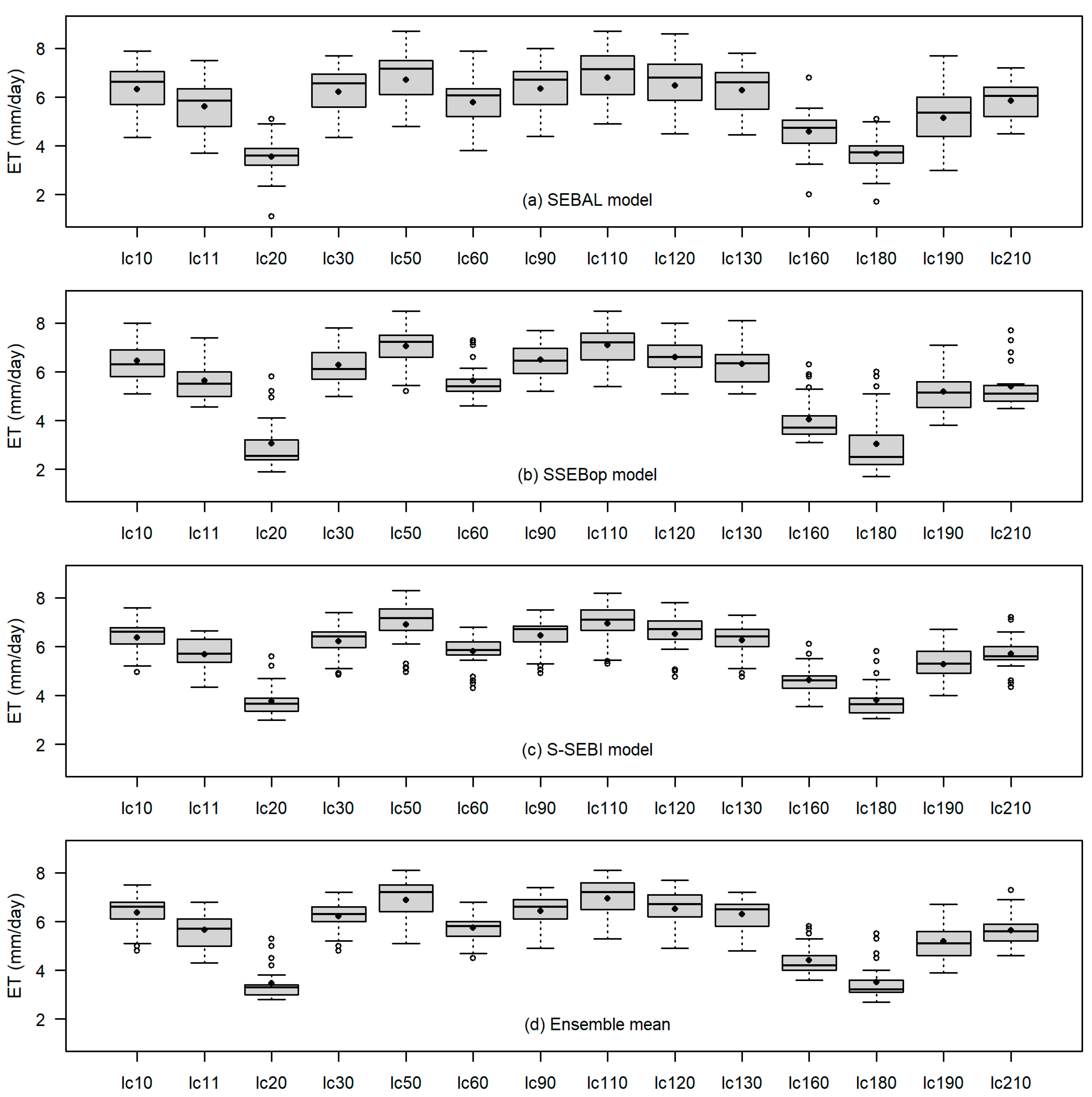
3.1. Actual ET Comparisons Based on Land Cover Classes

The ensemble mean of all Surface Energy Balance (SEB) models showed similar patterns in the mean daily evapotranspiration (ET) across all land cover classes (Figure 3). For example, mosaic herbaceous cover and broadleaved evergreen forest had the largest mean daily ET (Table 7). The higher mean daily ET for the evergreen forest was partly due to the relatively high moisture received by evergreen forest (regardless of the season) from the dense network of tributaries draining the mountains (both Udzungwa and Mbarika mountain ranges) where most of the evergreen forest is located. This finding was in line with Munishi-Kongo [81], who computed the daily ET across KV basin using the SEBS model [14] for four MODIS satellite overpasses (136th, 184th, 228th, and 303rd) during the dry season in 2010. S/he found that the evergreen forest had daily ET ranging between 6–8 mm regardless of the season. The relatively high ET over the mosaic herbaceous cover, which consists of large proportions of Miombo woodland, was attributed to the fact that the Miombo woodland maintains high ET rates due to its nature of maintaining leaves almost throughout the year, and starts leaf emergency some weeks before the rainfall onset [81]. These results suggest that all SEB models have managed to capture the actual ET ranges over these land cover classes.
All land cover classes located over the floodplain (post-flooding cropland, flooded tree cover, and flooded herbaceous cover) have a relatively low mean daily ET across all SEB models (Table 7). This was partly attributed by low soil moisture over the floodplain during the dry season. This suggestion is supported by Mombo et al. [82] who highlighted the dryness of the KV floodplain especially at the peak of the hot dry season in October. Fascinatingly, all models have managed to capture the expected relatively high ET (6.4 mm/day) over the cropland (Table 7). Cropland was expected to have higher ET due to dryland irrigation practiced in the area [24]. This result suggests the reliability of capturing real-life processes with the ET estimates derived by the SEB models used in this study.
The Wilcoxon’s test results (Table 8) show that the means of different pairs of SEB models across most of the land cover classes were statistically comparable (p-value > 0.05) with exception to land cover classes located over the flooded areas (land cover classes’ values 20, 160, and 180) and the water bodies (land cover class’s value 210) for the pairs of SEBAL vs. SSEBop, SSEBop vs. S-SEBI, and SSEBop vs. Ensemble Mean. The Levene’s test results (Table 8), on the other hand, show that the variances of different pairs of SEB models across different land cover classes were comparable (p-value > 0.05). Interestingly, the pairs of SEBAL vs. S-SEBI and SEBAL vs. Ensemble mean have p-values greater than 0.05 across all land cover classes, something which suggests the comparability of their ET estimates. It is noteworthy that whenever the Wilcoxon’ test and the Levene’s test give the opposite results (i.e., only one gives a p-value > 0.05), the test result for the variance (i.e., Levene’s test) is more robust than the test result for the mean (i.e., Wilcoxon’s test), therefore, a conclusion is made based on the Levene’s test [79].
By looking at performance metrics across different land use classes for different pairs of SEB model comparisons (Table 9), it is clear that all pairs of model comparisons performed reasonable well (r > 0.5) with the exception to the pair of SEBAL vs. SSEBop which have a relatively poor performance (r < 0.5) across most of the land cover classes. Fascinatingly, the pair of SEBAL vs. SSEBop performed well for the broadleaved evergreen (r = 0.68), mosaic herbaceous cover (r = 0.60) and shrubland (r = 0.54). Overall performance shows that all pair of models have biases less than 10% (Pbias < 10%) across all land cover classes with the exception to some of the pairs which contain the SSEBop model (e.g. SEBAL vs. SSEBop, SSEBop vs. S-SEBI, and SSEBop vs. Ensemble) for the land cover classes located over the flooded areas, namely, post-flooding cropland, flooded tree cover, and flooded herbaceous cover, respectively. Bhattarai et al. [38] reported the relatively poor performance of the SSEBop model compared to the SEBAL model over the marsh site (i.e., flooded area) in the humid (subtropical climate) southeastern United States.

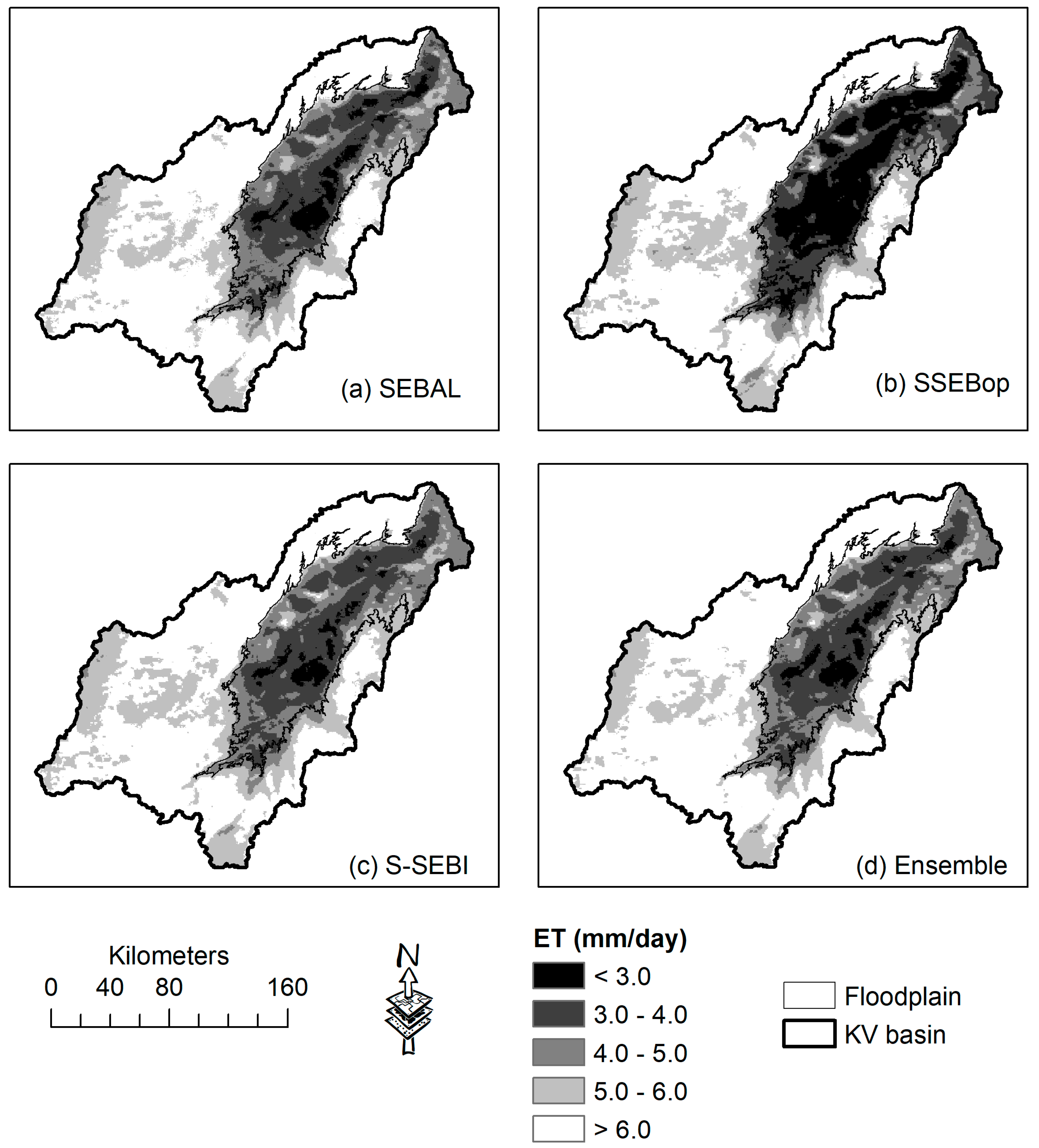
3.2. Graphical and Visual Comparisons of the Actual ET

All the SEB models were able to capture the two distinct ET regimes over the KV basin (Figure 4). The two distinct ET regimes can be distinguished as the relatively high ET regime over the mountainous parts of the basin and the areas across the periphery of the Valley bottom and the relatively low ET regime over the floodplain which comprises the Ramsar site (Kilombero Valley Floodplain). The two distinct ET regimes found in this study were in line with the findings from Munishi-Kongo [81] who performed snapshots (for the 136th, 184th, 228th, and 303rd days of the year in 2010) estimation of ET using MODIS satellite imagery and the Surface Energy Balance System (SEBS) model [14]. As aforementioned in Section 3.1, the relatively high ET regime over the mountainous area, in particular, can be partly attributed by the presence of the forests which receive moisture from the dense network of tributaries draining the mountains (both Udzungwa, and Mbarika mountain ranges) and orographic rainfall. On the other hand, the relatively low ET regime experienced by the floodplain was partly attributed by the dryness of the area (during the dry period) which partly, brought by seasonal crops which became dormant (i.e., low ET) after being harvested at the beginning of the dry season. This suggestion is supported by Mombo et al. [82] who attributed the dryness of wetlands in the Ramsar site with the high utilization of the wetlands in the KV basin.
Looking at the temporal dynamics of daily ET in the KV basin, it is clear that all the SEB models captured similar patterns of ET (Figure 5). Further exploration shows that the SEBAL model and the SSEBop model have relative larger variations of ET compared to the S-SEBI model and the ensemble mean of the three models. Interestingly, while the SEBAL model had a relatively low ET in the first data point compared to others, the SSEBop model had the highest ET. It is noteworthy that the temporal dynamics of ET shown in Figure 5 mimic the temporal dynamics of precipitation shown in Figure 2. This suggests that the temporal dynamics of ET in the KV river basin is partly controlled by the water availability in the basin. The temporal dynamics of ET estimates also captured the two distinct ET patterns (mountain-forests and wetland-valley) similar to those captured by the spatial dynamics in Figure 4. A close look at the temporal dynamics shows that the SSEBop model expresses the wet and dry seasons (Figure 5b). The overall trends of temporal dynamics show that there is no sharp boundary between the wet and the dry seasons in the basin. A similar pattern was reported by Koutsouris et al. [26] in their comparison of the global precipitation datasets across the Kilombero Valley.

3.3. Pre-Post SAGCOT Comparisons of the Actual ET

In 2010, the Tanzanian Government under the ‘Kilimo Kwanza’ (Agriculture first) policy launched an initiative entitled Southern Agriculture Corridor of Tanzania (SAGCOT) which aimed to ensure food security, and to improve the livelihood of people in Tanzania through expansion and intensification of agriculture in the southern parts of Tanzania which include the KV river basin [24]. As mentioned in the introduction, it becomes important to compare the ET estimates five years before and after the implementation of SAGCOT initiative to understand the impact of the SAGCOT initiative on the water consumption (via ET) in the basin.

Pre-post SAGCOT Comparisons across Land Cover Classes

There were relatively small decreases in the mean daily ET across all models for the land cover classes located over the floodplain (i.e., post-flooding cropland, flooded tree cover, and flooded herbaceous cover) (Table 10). The fact that the rest of the land cover classes showed a slight increase in the mean daily ET suggests that the decreased ET estimates over these land cover classes could partly be attributed by the expansion of cropland over these areas (i.e., between 2005 and 2015) which became dormant (i.e., low ET) after being harvested during the dry season of the year 2015 when the MODIS satellite overpasses were taken. When considering the magnitude of changes in ET across different models over these land cover classes, the SEBAL model had the lowest changes (−0.1 mm/day across all three land cover classes), and the SSEBop model had the highest changes (−0.5, −0.2, and −0.4 mm/day over the post-flooding cropland, flooded tree cover, and flooded herbaceous cover respectively). Exploration over the land cover classes with a slight increase in the ET estimates between 2005 and 2015 show the opposite trends (i.e., the SEBAL model had a relatively high ET and the SSEBop model had relatively low ET).
However, both the Wilcoxon’s test (which test differences in means) and the Levene’s test (which test differences in variances) results showed that any change in ET estimates across any land cover class for any SEB model was not statistically significant (i.e., p-value > 0.05) (Table 10). This suggests that the means and variances of ET estimates produced by either of the SEB models between 2005 and 2015 were statistically comparable. That is to say, the impact of implementing the SAGCOT initiative (in the mean daily actual ET estimates over different land cover classes) in the KV river basin was negligible based on these data.

4. Discussion

4.1. Implications for Sustainability of a Ramsar site (Kilombero Valley Floodplain)

Our results showing low actual ET estimates over the Kilombero floodplain are in line with the results obtained by Munishi-Kongo [81] that the floodplain actual ET is progressively declining in time as the season (of the year) changed from rainy (i.e., wet season) to dry (i.e., dry season). This partly implies the absence of actively growing vegetation over the floodplain areas towards the end of the dry season. The fact that the Kilombero Valley Floodplain (a Ramsar site) is located in the vicinity of the floodplain adds more concern as such a trend of ET over it during the dry season suggests the loss of habitat (wetland habitat) and decline in soil moisture. Mombo et al. [82] partly attributed this to the overexploitation (mainly cropland) of the Kilombero Valley Floodplain which resulted into the changing of status (from perennial streams into seasonal streams) of the Namawala, Kiberege, Kikwawila, Idete, and Idandu streams which used to supply water to the area, and the dry-up of many swamps within the wetland system. Further insights were given by Munishi-Kongo [81] who compared the daily ET over the wetland using the Landsat imagery and the SEBS model between two dates: 5 June 1991 (when the wetland had native vegetation) and 10 May 2002 (when wetland had bare land after the crops which replaced the native vegetation being harvested). S/he found a shift in the actual daily average ET from 3.5 mm/day (in 1991) to 1.2 mm/day (in 2002). The fact that both years (i.e., 1991 and 2002) had the same meteorological conditions (wet years with the mean annual rainfalls of 1447 mm and 1530 mm respectively), and both of the analyzed dates marked the beginning of the dry season, s/he attributed this substantial reduction of the actual ET (i.e., from 3.5 mm/day in 1991 to 1.2 mm/day in 2002) partly be due to the persistence of the former native vegetation to withstand dry conditions (i.e., relatively high ET) compared to the bare land (low ET) brought by the harvested crops which replaced the former native vegetation. This suggests that the extensive utilization of the Kilombero floodplain (especially the Kilombero Valley Floodplain) by anthropogenic activities (e.g., agriculture) might threaten the sustainability of the eco-hydrological system of the Ramsar site (Kilombero Valley Floodplain) which is an important habitat of various species of flora and fauna (specific names of these species can be found in Seki et al. [83]).
A study on the impact of land use and cover change (LULC) on biodiversity around Kilombero Valley Floodplain done by Seki et al. [83] using forty-eight vegetation survey plots (0.08 ha) combined with Landsat imagery (1990, 1998, and 2011) revealed a significant change in LULC in the area with anthropogenic activities being the main trigger of such changes. They found out that a large area of open water was covered by floating sedges coming from increased sediments into the wetland. In addition, they found strong evidence on the modification of the structure and functioning of ecosystem services and the loss of species due to LULC changes. They concluded that their study by underlining the vulnerability of the wetland system due to anthropogenic degradation and recommended the monitoring programs to ensure sustainable utilization of the Kilombero Valley Floodplain.

4.2. On the Applicability of the Approach

Our approach of evaluating estimates of hydrological variable (such as ET and precipitation) derived from one model with the corresponding estimates derived from another model is a widely used (as standard approach) approach, especially in the data-limited regions where information on hydrological variables are highly needed for informed decision making, but their availability is often limited by scarcity, gaps, and/or discrepancies. For example, Kiptala et al. [4], and Alemayehu et al. [5] have compared the ET estimates derived using their SEBAL and SSEBop models, respectively, with ET estimates derived from another remote sensing based ET estimation algorithm, namely, the MODIS 16 algorithm [53] in the Upper Pangani river basin (Tanzania/Kenya) and the Mara river basin (Tanzania/Kenya). Alemu et al. [84] analyzed the performance of the ET estimates derived from SSEBop model, and MODIS 16 algorithm [53] using the Tropical Rainfall Measuring Mission (TRMM) multi-satellite precipitation analysis dataset over the Nile basin. Elsewhere Velpuri et al. [85] compared ET estimates derived using the SSEBop model [17] to that derived via the MODIS 16 algorithm [53] over the data-rich conterminous United States. Their study also involves a comprehensive evaluation of these two ET estimates using point and gridded FLUXNET and water balance ET. A similar approach has been widely used to compare global precipitation datasets. For example, Koutsouris et al. [26] evaluated the performance of seven global precipitation data sets (GPDs) against the Tropical Rainfall Measuring Mission (TRMM) multi-satellite precipitation analysis research-grade product v7 (TRMMv7) in the hydro-climatic data-limited Kilombero Valley (KV) basin. Specific names of these seven GDPs can be found in Koutsouris et al. [26]. They recommend their approach to be used to provide guidance to the choice of GPDs for water resources management in data poor regions. Therefore, it is clear that a similar approach can be utilized to provide guidance to the choice of ET estimates for water resources management and to constrain (or to evaluate performance of) the hydrological model (e.g., in Alemayehu et al. [86], Immerzeel and Droogers [87], and Winsemius et al., 2008 [88]).

4.3. On Limitations and Potential Uncertainties of ET Estimates

Surface energy balance (SEB) ET models driven by remote sensing (RS) data and various meteorological data have uncertainties due to inevitable input (driving/forcing) errors, poorly defined model parameters, insufficient model structures [74,89], and the technical skills of the operator/modeler [18]. The latter (i.e., modeler’s skills) holds true especially due to the fact that the application of SEB to a wide heterogeneous area with a complex mixture of agricultural crops and other vegetation involves considerable empiricism which calls for local refinement. This not only requires a modeler with knowledge of the study area, but also a strong physics background on the top of high-quality input data [18]. Therefore, SEB models should be operated only by people with special skills.
As we have highlighted in the preceding section, one of the main sources of uncertainties in the application of the SEBAL model is the selection of the cold and the hot pixels (i.e., the anchor pixels) especially for the coarse satellite imagery such as MODIS-based images (250 m for this study compared to 30 m of Landsat). Allen et al. [61] pointed out the difficulty in finding homogenous vegetation with sufficient ground cover to represent the cold pixel using the MODIS image. Long et al. [90] found that an increase in temperatures of cold and hot pixels increased LE and reduced H, and vice versa. An approach used to estimate aerodynamic stability correction and surface roughness might also be a source of biases in the SEBAL model [18]. An idea of ignoring the daily Soil Heat flux ( G 24 ) by assuming the night and day balance might also lead to uncertainty. In addition, there are potential biases and uncertainties inherent from quantification of the net radiation ( R n ) and the soil heat flux ( G ) regardless of the efforts made to compute each of them as unbiased and as accurately as possible [61]. Even though the SEBAL model attempts to cancel the inherent biases to R n and G through internal calibration using the Monin–Obkhuv schemes when estimating the sensible heat flux ( H ), still several SEBAL model studies reported an underestimation of H under dry conditions which, in turn, overestimates the actual ET [38,40]. Gokmen et al. [91] and Van De Kwast et al. [47] also reported the same concern from their respective ET estimation studies using the Surface Energy Balance System (SEBS) model [14]. For example, Gokmen et al. [91] attributed such an underestimation (of H) with the fact that most SEB models do not explicitly consider the soil moisture dependency, instead, they assume that the variation in RS-based variables such as surface temperature ( T s ) and Normalized Difference Vegetation Index ( N D V I ) account for changes in soil moisture, something which causes uncertainty in the estimated H.
The sensitivity analysis performed by Chen at al. [74] found that, the SSEBop model is most sensitive to input variables: T s , and the reference evapotranspiration ( E T 0 ), and model parameters: the predefined differential temperature ( d T ), and the maximum ET scaling factor ( k m a x ), especially, during the non-growing season and in dry areas. They suggested the possibility of improving the SSEBop model ET estimates by reducing errors in these input variables (i.e., T s and E T 0 ) and model parameters (i.e., d T and k m a x ). Bhattarai et al. [38] associated the weak performance of the SSEBop model (as compared to the other four SEB models, namely, SEBAL, S-SEBI, SEBS, and METRIC) with the overestimation of the hypothetical cold temperature ( T c o l d ) which was partly attributed with the constant calibration coefficient ( c ) used to estimate the T c o l d . The current study adopted the approach used by Alemayehu et al. [5] who used a seasonally-varying c as proposed by Senay et al. [17]. Like Chen et al. [74], Bhattarai et al. [38] also found uncertainty in the estimation of a predefined d T , and they partly attributed it with the assumption adopted by the SSEBop model that surface roughness ( r a h ) is constant ( r a h = 110 s/m) for all pixels throughout the image. To encounter this shortcoming, a local calibration or some analytical/physical formulations should be incorporated into the SSEBop model parameterization to account for the spatial and temporal variations in r a h .
Lastly, the main source of uncertainty in the model structure of the S-SEBI model [19] is the assumption adopted in the establishment of the trapezoidal space (i.e., linearity of surface temperature ( T s ) and albedo ( α )) used to define the two extreme conditions (i.e., the cold edge which determines the cold reference temperature ( T c o l d ), and the hot edge which determines the hot reference temperature ( T h o t )). For example, to account for such uncertainty, Bhattarai et al. [38] ignored all T s values outside the range of T c o l d , s e b a l 10 K and T h o t , s e b a l + 20 K , where T c o l d , s e b a l and T h o t , s e b a l are T s values used for anchor pixels in the SEBAL model. Interestingly, they did not report any improvement in the actual ET estimates resulting from such modification.
It is noteworthy to point out that the model simplification adopted by the partial SEB models such as the S-SEBI model does not necessarily render them to be less accurate than more complex full SEB models such as the SEBAL model [92]. McCabe et al. [89] noted that data-intensive, physically-based SEB models such as the SEBS model [14] are more sensitive to the quality of the input data than SEB models with fewer inputs. For example, Wagle et al. [40] computed the daily ET estimates in the high biomass sorghum in Oklahoma, United States (US) and found out that the S-SEBI model performed relatively better than the SEBAL and the SEBS models. Fascinatingly, other SEB models comparison studies by Bhattarai et al. [38] over four sites, namely, grass, citrus, marsh, and open water in the humid southeastern US found out that the S-SEBI model came third in performance after the SEBS and the SEBAL models. These interesting opposite results seem to support our idea of comparing ET estimates derived from different SEB models and select ET estimates for further applications (such as hydrological modeling) based on their similarities and contrasts.

4.4. Implications for Hydrological Modeling

Considering the difficulty of comparing snapshots of RS products to derive trends (or to see the impacts of SAGCOT on the landscape) and the need for decision support tools to secure sustainability, the results of this study show that the actual ET estimates derived from SEB models could be used in both distributed and lumped hydrological models in this region. This is attributed by the consistency of the mean of ET estimates computed by different SEB models in a given spatial scale (the entire basin, mountain-forests, and wetland-valley). The actual ET estimates can be used either to constrain the hydrological model or as a model evaluation variable for model calibration and/or validation. For example, Parajuli et al. [93] used monthly ET estimates from SEBAL model using MODIS datasets to evaluate the performance of the SWAT model in 2 sub-basins (Merigold and Sunflower) within the Big Sunflower River Watershed (BSRW) in Northwestern, Mississippi. They obtained good model performances with the coefficient of determination (R2) and Nash-Sutcliffe Efficiency (NSE) ranging from 0.79 to 0.82 during model calibration, and 0.71 to 0.78 during model validation. Their study results demonstrated the applicability of ET estimates derived from SEB models using MODIS-based remote sensing data to evaluate the hydrological model, something which is useful in hydrological basins with hydrometeorological data scarcity such as those located in the global south which includes the KV river basin. Kiptala et al. [94] used remote-sensing-based ET estimates generated using MODIS satellite datasets and the SEBAL model in a heterogeneous, heavily utilized, and data-limited upper Pangani river basin (Tanzania/Kenya) to constrain (i.e., input data) a distributed hydrological model, namely, the Spatial Tools for River Basin Environmental Analysis and Management (STREAM) model [95]. They calibrated their model using streamflow data at an 8-day temporal resolution and obtained a Nash–Sutcliffe Efficiency of the natural logarithm (which emphasizes the base flow) of 0.9 at the basin’s outlet. This good model performance signifies the applicability of the remote-sensed ET estimates to constrain the hydrological model. Cheema et al. [96] used the actual ET estimates from ETLook to calibrate the SWAT model parameterized using satellite-based rainfall to quantify the contribution of groundwater (GW) use in the Indus river basin, Asia. Recently, Wambura et al. [97] used the spatial patterns of average ET as one of the constraints (others were streamflow, shallow GW level, and land cover change) to investigate the reduction of equifinality (i.e., multiple feasible descriptions of hydrological processes) and prediction uncertainty in the SWAT model in the Wami river basin, Tanzania. They found out that the incorporation of additional constraints (on top of conventional streamflow) produced consistent performance with respect to the hydrograph than that of the classical (conventional) hydrological modeling without additional constraints. This implies that the inclusion of ET patterns in their distributed model (SWAT model) substantially minimizes equifinality and prediction uncertainty in the model.
However, there are various challenges that tend to limit applications of remote sensing (RS) data (including ET) on hydrological modeling. Some of these challenges include (a) the limited availability of satellite data (i.e., RS data) at a reasonable scale (spatial and/or temporal) to capture dominant hydrological processes in the hydrological basin. For example, Landsat has a high spatial resolution (30 m), but with low temporal resolution (16-day). MODIS, on the other hand, has a high temporal resolution (up to daily), but with a low spatial resolution (from 250 m); (b) limited flexibility to incorporate spatially distributed RS data into the hydrological model. This holds true, especially with the hydrological model which the user lacks control in editing the model code/structure (such as the Systeme Hydrologique European (SHE) model [98]). This means that the user is limited to optimize model performance using secondary data such as RS-derived ET. (c) limited technical skills by modelers to convert RS data into hydrometeorological data [99]. This lack of technical skills suggests the limitation of modeler/hydrologist to come up with a hydrological model capable of representing the dominant hydrological process, like the conceptual model framework proposed by Savenije [100]. Readers are recommended to refer to Schultz [99] for more details on the opportunities and challenges of the utilization of RS in hydrological modeling. Appropriate technical skills on how to utilize secondary data from RS to calibrate or infer model parameters have enabled various researchers to improve the robustness of their respective hydrological models [88,101,102].

5. Conclusions

This study has applied three different remote-sensing (RS) based Surface Energy Balance (SEB) models—the Surface Energy Balance Algorithm for Land (SEBAL) model, the Operational Simplified Surface Energy Balance (SSEBop) model, and the Simplified Surface Balance Index (S-SEBI) model—to estimate spatially-distributed evapotranspiration (ET) rates across the Kilombero Valley (KV) river basin in Tanzania for multiple days in three different years—2005, 2010, and 2015. The main purpose of the study is to evaluate similarities and differences in the SEB models and also to evaluate differences in time in the ET rates as irrigation and land use changed over time.
Our results show that all the SEB models showed similar patterns in the mean daily ET estimates across all land cover classes. For example, mosaic herbaceous cover had the largest mean daily ET, 6.8 ± 1.1 mm/day, 7.1 ± 0.9 mm/day, 6.9 ± 0.8 mm/day, and 6.9 ± 0.8 mm/day for the SEBAL, SSEBop, S-SEBI, and the ensemble mean, respectively. All the SEB models were able to capture the two distinct ET regimes over the study area: the relatively high ET regime over the mountainous parts of the basin and the areas across the periphery of the Valley bottom. The SEB models could also capture the relatively low ET regime over the floodplain which comprises a Ramsar site, namely, the Kilombero Valley Floodplain. The relatively high ET regime over the mountainous can be partly attributed by the presence of the forests which receive moisture from the dense network of tributaries draining the mountains (both Udzungwa, and Mbarika mountain ranges) and orographic rainfall. The relatively low ET regime experienced by the floodplain can be partly attributed by the dryness of the area (during the dry period) which were partly brought by seasonal crops which became dormant (i.e., low ET) after being harvested at the beginning of the dry season. Statistical analysis showed that the pair of the SEBAL model versus the SSEBop model has the worst results with the correlation coefficient (r), less than 0.5 across most of the land covers. However, the relative high correlation coefficient (r) across the broadleaved evergreen (r = 0.68), mosaic herbaceous cover (r = 0.60) and shrubland (r = 0.54) together with the percent bias (Pbias) of less than 10% across most of the land covers preclude disqualification of this pair. Overall results suggest that the mean of the ensemble is a better representation of the SEB models in the study area. It is worth noting that this suggestion may have been specific to the circumstances (e.g., the external conditions) in which the models were being used.
The potential limitation of this present study was the absence of independent measurements against which to compare the modeled ET rates. However, our approach of evaluating ET estimates derived from one model with the ET estimates derived from another model is a widely used (as standard approach) approach to tackle such limitation. This is especially true in data-limited regions where information on hydrological variables are needed for informed decision making, but their availability is often limited by scarcity, gaps, and/or discrepancies.

Author Contributions

W.S. conceived, designed, analyzed and wrote the paper. S.E.M., M.T. and J.N. reviewed the paper and contributed to writing. S.W.L. supervised the research, contributed ideas during interpretation and writing the paper.

Funding

This research was funded by the Swedish International Development Agency (Sida) under Grant SWE-2011-066 and Sida Decision 2015-000032 Contribution 51170071 Sub-project 2239.

Acknowledgments

We acknowledge the efforts made by editors and three anonymous reviewers to improve the presentation and the clarity of this work.

Conflicts of Interest

The authors declare no conflict of interest.

References

  1. Katul, G.G.; Oren, R.; Manzoni, S.; Higgins, C.; Parlange, M.B. Evapotranspiration: A process driving mass transport and energy exchange in the soil-plant-atmosphere-climate system. Rev. Geophys. 2012, 50, RG3002. [Google Scholar] [CrossRef]
  2. Oki, T.; Kanae, S. Global hydrological cycles and world water resources. Science 2006, 313, 1068–1072. [Google Scholar] [CrossRef] [PubMed]
  3. Burba, G.G.; Verma, S.B. Seasonal and interannual variability in evapotranspiration of native tallgrass prairie and cultivated wheat ecosystems. Agric. For. Meteorol. 2005, 135, 190–201. [Google Scholar] [CrossRef]
  4. Kiptala, J.K.; Mohamed, Y.; Mul, M.L.; Van Der Zaag, P. Mapping evapotranspiration trends using MODIS and SEBAL model in a data scarce and heterogeneous landscape in Eastern Africa. Water Resour. Res. 2013, 49, 8495–8510. [Google Scholar] [CrossRef] [Green Version]
  5. Alemayehu, T.; van Griensven, A.; Senay, G.B.; Bauwens, W. Evapotranspiration Mapping in a Heterogeneous Landscape Using Remote Sensing and Global Weather Datasets: Application to the Mara Basin, East Africa. Remote Sens. 2017, 9, 390. [Google Scholar] [CrossRef]
  6. Anderson, M.C.; Norman, J.M.; Mecikalski, J.R.; Otkin, J.A.; Kustas, W.P. A climatological study of evapotranspiration and moisture stress across the continental United States based on thermal remote sensing: 1. Model formulation. J. Geophys. Res. Atmos. 2007, 112, D10117. [Google Scholar] [CrossRef]
  7. Bastiaanssen, W.G.M.; Ahmad, M.-U.-D.; Chemin, Y. Satellite surveillance of evaporative depletion across the Indus Basin. Water Resour. Res. 2002, 38, 91–99. [Google Scholar] [CrossRef]
  8. Allen, R.G.; Pereira, L.S.; Howell, T.A.; Jensen, M.E. Evapotranspiration information reporting: II. Recommended documentation. Agric. Water Manag. 2011, 98, 921–929. [Google Scholar] [CrossRef]
  9. Jaramillo, F.; Destouni, G. Developing water change spectra and distinguishing change drivers worldwide. Geophys. Res. Lett. 2014, 41, 8377–8386. [Google Scholar] [CrossRef]
  10. Yang, Y.; Shang, S.; Jiang, L. Remote sensing temporal and spatial patterns of evapotranspiration and the responses to water management in a large irrigation district of North China. Agric. For. Meteorol. 2012, 164, 112–122. [Google Scholar] [CrossRef]
  11. Baldocchi, D.D. Assessing the eddy covariance technique for evaluating carbon dioxide exchange rates of ecosystems: Past, present and future. Glob. Chang. Biol. 2003, 9, 479–492. [Google Scholar] [CrossRef]
  12. Wright, J.L. New evapotranspiration crop coefficients. J. Irrig. Drain. Div. ASCE 1982, 108, 57–74. [Google Scholar]
  13. Zhang, B.; Kang, S.; Li, F.; Zhang, L. Comparison of three evapotranspiration models to Bowen ratio-energy balance method for a vineyard in an arid desert region of northwest China. Agric. For. Meteorol. 2008, 148, 1629–1640. [Google Scholar] [CrossRef]
  14. Su, Z. The Surface Energy Balance System (SEBS) for estimation of turbulent heat fluxes. Hydrol. Earth Syst. Sci. 2002, 6, 85–99. [Google Scholar] [CrossRef]
  15. Li, Z.-L.; Tang, R.; Wan, Z.; Bi, Y.; Zhou, C.; Tang, B.; Yan, G.; Zhang, X. A review of current methodologies for regional Evapotranspiration estimation from remotely sensed data. Sensors 2009, 9, 3801–3853. [Google Scholar] [CrossRef]
  16. Bastiaanssen, W.G.M.; Menenti, M.; Feddes, R.A.; Holtslag, A.A.M. A remote sensing surface energy balance algorithm for land (SEBAL): 1. Formulation. J. Hydrol. 1998, 212–213, 198–212. [Google Scholar] [CrossRef]
  17. Senay, G.B.; Bohms, S.; Singh, R.K.; Gowda, P.H.; Velpuri, N.M.; Alemu, H.; Verdin, J.P. Operational Evapotranspiration Mapping Using Remote Sensing and Weather Datasets: A New Parameterization for the SSEB Approach. J. Am. Water Resour. Assoc. 2013, 49, 577–591. [Google Scholar] [CrossRef] [Green Version]
  18. Allen, R.G.; Tasumi, M.; Trezza, R. Satellite-based energy balance for mapping evapotranspiration with internalized calibration (METRIC)—Model. J. Irrig. Drain. Eng. 2007, 133, 380–394. [Google Scholar] [CrossRef]
  19. Roerink, G.J.; Su, Z.; Menenti, M. S-SEBI: A simple remote sensing algorithm to estimate the surface energy balance. Phys. Chem. Earth Part B Hydrol. Oceans Atmos. 2000, 25, 147–157. [Google Scholar] [CrossRef]
  20. Gowda, P.H.; Chavez, J.L.; Colaizzi, P.D.; Evett, S.R.; Howell, T.A.; Tolk, J.A. ET mapping for Agric. Water Manag.: Present status and challenges. Irrig. Sci. 2008, 26, 223–237. [Google Scholar] [CrossRef]
  21. Karimi, P.; Bastiaanssen, W.G.M. Spatial evapotranspiration, rainfall and land use data in water accounting—Part 1: Review of the accuracy of the remote sensing data. Hydrol. Earth Syst. Sci. 2015, 19, 507–532. [Google Scholar] [CrossRef]
  22. Monin, A.S.; Obukhov, A.M. Basic laws of turbulent mixing in the surface layer of the atmosphere. Tr. Akad. Nauk SSSR Geophiz. Inst. 1954, 24, 163–187. [Google Scholar]
  23. Bastiaanssen, W.G.M.; Noordman, E.J.M.; Pelgrum, H.; Davids, G.; Thoreson, B.P.; Allen, R.G. SEBAL model with remotely sensed data to improve water-resources management under actual field conditions. J. Irrig. Drain. Eng. 2005, 131, 85–93. [Google Scholar] [CrossRef]
  24. Senkondo, W.; Tumbo, M.; Lyon, S.W. On the evolution of hydrological modelling for water resources in Eastern Africa. CAB Rev. 2018, 13, 1–26. [Google Scholar] [CrossRef]
  25. Alavaisha, E.; Lyon, S.W.; Lindborg, R. Assessment of Water Quality across Irrigation Schemes: A Case Study of Wetland Agriculture Impacts in Kilombero Valley, Tanzania. Water (Switzerland) 2019, 11, 671. [Google Scholar] [CrossRef]
  26. Koutsouris, A.J.; Chen, D.; Lyon, S.W. Comparing global precipitation data sets in eastern Africa: A case study of Kilombero Valley, Tanzania. Int. J. Climatol. 2016, 36, 2000–2014. [Google Scholar] [CrossRef]
  27. Koutsouris, A.J.; Lyon, S.W. Advancing understanding in data-limited conditions: Estimating contributions to streamflow across Tanzania’s rapidly developing kilombero valley. Hydrol. Sci. J. 2018, 63, 197–209. [Google Scholar] [CrossRef]
  28. Näschen, K.; Diekkrüger, B.; Leemhuis, C.; Steinbach, S.; Seregina, L.S.; Thonfeld, F.; van der Linden, R. Hydrological modeling in data-scarce catchments: The Kilombero floodplain in Tanzania. Water (Switzerland) 2018, 10, 599. [Google Scholar] [CrossRef]
  29. Lyon, S.W.; Koutsouris, A.; Scheibler, F.; Jarsjo, J.; Mbanguka, R.; Tumbo, M.; Robert, K.K.; Sharma, A.N.; van der Velde, Y. Interpreting characteristic drainage timescale variability across Kilombero Valley, Tanzania. Hydrol. Process. 2015, 29, 1912–1924. [Google Scholar] [CrossRef]
  30. Bonarius, H. Physical Properties of Soils in the Kilombero Valley (Tanzania); German Agency for Technical Cooperation (GTZ): Eschborn, Germany, 1975; p. 36.
  31. Leemhuis, C.; Thonfeld, F.; Näschen, K.; Steinbach, S.; Muro, J.; Strauch, A.; López, A.; Daconto, G.; Games, I.; Diekkrüger, B. Sustainability in the food-water-ecosystem nexus: The role of land use and land cover change for water resources and ecosystems in the Kilombero Wetland, Tanzania. Sustainability (Switzerland) 2017, 9, 1513. [Google Scholar] [CrossRef]
  32. Beck, A.D. The Kilombero valley of South-Central Tanganyika. East Afr. Geograph. Rev. 1964, 2, 37–43. [Google Scholar]
  33. Senkondo, W.; Tuwa, J.; Koutsouris, A.; Tumbo, M.; Lyon, S.W. Estimating aquifer transmissivity using the recession-curve-displacement method in Tanzania’s Kilombero valley. Water (Switzerland) 2017, 9, 948. [Google Scholar] [CrossRef]
  34. McClain, M.E.; Williams, K. Environmental Flows in Rufiji River Basin Assessed from the Perspective of Planned Development in Kilombero and Lower Rufiji Sub-Basins; CDM International, Inc. (CDM Smith): Boston, MA, USA, 2016; p. 148. [Google Scholar]
  35. Burghof, S.; Gabiri, G.; Stumpp, C.; Chesnaux, R.; Reichert, B. Development of a hydrogeological conceptual wetland model in the data-scarce north-eastern region of Kilombero Valley, Tanzania. Hydrogeol. J. 2018, 26, 267–284. [Google Scholar] [CrossRef]
  36. Dewitte, O.; Jones, A.; Spaargaren, O.; Breuning-Madsen, H.; Brossard, M.; Dampha, A.; Deckers, J.; Gallali, T.; Hallett, S.; Jones, R.; et al. Harmonisation of the soil map of africa at the continental scale. Geoderma 2013, 211–212, 138–153. [Google Scholar] [CrossRef]
  37. Al Zayed, I.S.; Elagib, N.A.; Ribbe, L.; Heinrich, J. Satellite-based evapotranspiration over Gezira Irrigation Scheme, Sudan: A comparative study. Agric. Water Manag. 2016, 177, 66–76. [Google Scholar] [CrossRef]
  38. Bhattarai, N.; Shaw, S.B.; Quackenbush, L.J.; Im, J.; Niraula, R. Evaluating five remote sensing based single-source surface energy balance models for estimating daily evapotranspiration in a humid subtropical climate. Int. J. Appl. Earth Observ. Geoinf. 2016, 49, 75–86. [Google Scholar] [CrossRef]
  39. Singh, R.K.; Senay, G.B. Comparison of four different energy balance models for estimating EvapoTranspiration in the Midwestern United States. Water (Switzerland) 2016, 8, 9. [Google Scholar] [CrossRef]
  40. Wagle, P.; Bhattarai, N.; Gowda, P.H.; Kakani, V.G. Performance of five surface energy balance models for estimating daily evapotranspiration in high biomass sorghum. ISPRS J. Photogramm. Remote Sens. 2017, 128, 192–203. [Google Scholar] [CrossRef] [Green Version]
  41. Kite, G.W.; Droogers, P. Comparing evapotranspiration estimates from satellites, hydrological models and field data. J. Hydrol. 2000, 229, 3–18. [Google Scholar] [CrossRef]
  42. Mohamed, Y.A.; Bastiaanssen, W.G.M.; Savenije, H.H.G. Spatial variability of evaporation and moisture storage in the swamps of the upper Nile studied by remote sensing techniques. J. Hydrol. 2004, 289, 145–164. [Google Scholar] [CrossRef]
  43. Mahmoud, S.H.; Alazba, A.A. A coupled remote sensing and the Surface Energy Balance based algorithms to estimate actual evapotranspiration over the western and southern regions of Saudi Arabia. J. Asian Earth Sci. 2016, 124, 269–283. [Google Scholar] [CrossRef]
  44. Sun, Z.; Wei, B.; Su, W.; Shen, W.; Wang, C.; You, D.; Liu, Z. Evapotranspiration estimation based on the SEBAL model in the Nansi Lake Wetland of China. Math. Comput. Model. 2011, 54, 1086–1092. [Google Scholar] [CrossRef]
  45. Justice, C.O.; Townshend, J.R.G.; Vermote, E.F.; Masuoka, E.; Wolfe, R.; Saleous, N.; Roy, D.P.; Morisette, J.T. An overview of MODIS Land data processing and product status. Remote Sens. Environ. 2002, 83, 3–15. [Google Scholar] [CrossRef]
  46. Roy, D.P.; Borak, J.S.; Devadiga, S.; Wolfe, R.E.; Zheng, M.; Descloitres, J. The MODIS Land product quality assessment approach. Remote Sens. Environ. 2002, 83, 62–76. [Google Scholar] [CrossRef]
  47. Van Der Kwast, J.; Timmermans, W.; Gieske, A.; Su, Z.; Olioso, A.; Jia, L.; Elbers, J.; Karssenberg, D.; De Jong, S. Evaluation of the Surface Energy Balance System (SEBS) applied to ASTER imagery with flux-measurements at the SPARC 2004 site (Barrax, Spain). Hydrol. Earth Syst. Sci. 2009, 13, 1337–1347. [Google Scholar] [CrossRef] [Green Version]
  48. Colditz, R.R.; Conrad, C.; Wehrmann, T.; Schmidt, M.; Dech, S. TiSeG: A flexible software tool for time-series generation of MODIS data utilizing the quality assessment science data set. IEEE Trans. Geosci. Remote Sens. 2008, 46, 3296–3308. [Google Scholar] [CrossRef]
  49. Tang, R.; Li, Z.-L.; Chen, K.-S.; Jia, Y.; Li, C.; Sun, X. Spatial-scale effect on the SEBAL model for evapotranspiration estimation using remote sensing data. Agric. For. Meteorol. 2013, 174–175, 28–42. [Google Scholar] [CrossRef]
  50. Conrad, C.; Dech, S.W.; Hafeez, M.; Lamers, J.; Martius, C.; Strunz, G. Mapping and assessing water use in a Central Asian irrigation system by utilizing MODIS remote sensing products. Irrig. Drain. Syst. 2007, 21, 197–218. [Google Scholar] [CrossRef] [Green Version]
  51. Hijmans, R.J. Raster: Geographic Analysis and Modeling with Raster Data. R Package Version 2.8-4. Available online: https://cran.r-project.org/web/packages/raster/ (accessed on 14 December 2018).
  52. Weiss, D.J.; Atkinson, P.M.; Bhatt, S.; Mappin, B.; Hay, S.I.; Gething, P.W. An effective approach for gap-filling continental scale remotely sensed time-series. ISPRS J. Photogramm. Remote Sens. 2014, 98, 106–118. [Google Scholar] [CrossRef] [PubMed] [Green Version]
  53. Mu, Q.; Zhao, M.; Running, S.W. Improvements to a MODIS global terrestrial evapotranspiration algorithm. Remote Sens. Environ. 2011, 115, 1781–1800. [Google Scholar] [CrossRef]
  54. Zeng, C.; Shen, H.; Zhang, L. Recovering missing pixels for Landsat ETM+ SLC-off imagery using multi-temporal regression analysis and a regularization method. Remote Sens. Environ. 2013, 131, 182–194. [Google Scholar] [CrossRef]
  55. Zhao, M.; Heinsch, F.A.; Nemani, R.R.; Running, S.W. Improvements of the MODIS terrestrial gross and net primary production global data set. Remote Sens. Environ. 2005, 95, 164–176. [Google Scholar] [CrossRef]
  56. Teixeira, A.H.d.C.; Bastiaanssen, W.G.M.; Ahmad, M.D.; Bos, M.G. Reviewing SEBAL input parameters for assessing evapotranspiration and water productivity for the Low-Middle São Francisco River basin, Brazil. Part A: Calibration and validation. Agric. For. Meteorol. 2009, 149, 462–476. [Google Scholar] [CrossRef]
  57. Chen, H.; Huo, Z.; Dai, X.; Ma, S.; Xu, X.; Huang, G. Impact of agricultural water-saving practices on regional evapotranspiration: The role of groundwater in sustainable agriculture in arid and semi-arid areas. Agric. For. Meteorol. 2018, 263, 156–168. [Google Scholar] [CrossRef]
  58. French, A.N.; Jacob, F.; Anderson, M.C.; Kustas, W.P.; Timmermans, W.; Gieske, A.; Su, Z.; Su, H.; McCabe, M.F.; Li, F.; et al. Surface energy fluxes with the Advanced Spaceborne Thermal Emission and Reflection radiometer (ASTER) at the Iowa 2002 SMACEX site (USA). Remote Sens. Environ. 2005, 99, 55–65. [Google Scholar] [CrossRef]
  59. Long, D.; Singh, V.P. Assessing the impact of end-member selection on the accuracy of satellite-based spatial variability models for actual evapotranspiration estimation. Water Resour. Res. 2013, 49, 2601–2618. [Google Scholar] [CrossRef]
  60. Wang, Z.; Mao, D.; Li, L.; Jia, M.; Dong, Z.; Miao, Z.; Ren, C.; Song, C. Quantifying changes in multiple ecosystem services during 1992–2012 in the Sanjiang Plain of China. Sci. Total Environ. 2015, 514, 119–130. [Google Scholar] [CrossRef] [PubMed]
  61. Allen, R.; Irmak, A.; Trezza, R.; Hendrickx, J.M.H.; Bastiaanssen, W.; Kjaersgaard, J. Satellite-based ET estimation in agriculture using SEBAL and METRIC. Hydrol. Process. 2011, 25, 4011–4027. [Google Scholar] [CrossRef]
  62. Zhou, Y.; Li, X.; Yang, K.; Zhou, J. Assessing the impacts of an ecological water diversion project on water consumption through high-resolution estimations of actual evapotranspiration in the downstream regions of the Heihe River Basin, China. Agric. For. Meteorol. 2018, 249, 210–227. [Google Scholar] [CrossRef]
  63. Bastiaanssen, W.G.M. SEBAL-based sensible and latent heat fluxes in the irrigated Gediz Basin, Turkey. J. Hydrol. 2000, 229, 87–100. [Google Scholar] [CrossRef]
  64. Farah, H.O.; Bastiaanssen, W.G.M. Impact of spatial variations of land surface parameters on regional evaporation: A case study with remote sensing data. Hydrol. Process. 2001, 15, 1585–1607. [Google Scholar] [CrossRef]
  65. Owusu, G. Sebkc: The Surface Energy Balance and Crop Coefficient Estimation with R. R Package Version 1.0-1. Available online: https://rdrr.io/github/gowusu/sebkc/ (accessed on 14 December 2018).
  66. Allen, R.G.; Burnett, B.; Kramber, W.; Huntington, J.; Kjaersgaard, J.; Kilic, A.; Kelly, C.; Trezza, R. Automated calibration of the METRIC-Landsat evapotranspiration process. J. Am. Water Resources Assoc. 2013, 49, 563–576. [Google Scholar] [CrossRef]
  67. Bhattarai, N.; Quackenbush, L.J.; Im, J.; Shaw, S.B. A new optimized algorithm for automating endmember pixel selection in the SEBAL and METRIC models. Remote Sens. Environ. 2017, 196, 178–192. [Google Scholar] [CrossRef]
  68. Brutsaert, W.; Sugita, M. Application of self-preservation in the diurnal evolution of the surface energy budget to determine daily evaporation. J. Geophys. Res. 1992, 97, 18377–18382. [Google Scholar] [CrossRef]
  69. Farah, H.O.; Bastiaanssen, W.G.M.; Feddes, R.A. Evaluation of the temporal variability of the evaporative fraction in a tropical watershed. Int. J. Appl. Earth Observ. Geoinf. 2004, 5, 129–140. [Google Scholar] [CrossRef]
  70. Peng, J.; Borsche, M.; Liu, Y.; Loew, A. How representative are instantaneous evaporative fraction measurements of daytime fluxes? Hydrol. Earth Syst. Sci. 2013, 17, 3913–3919. [Google Scholar] [CrossRef]
  71. Singh, R.K.; Irmak, A.; Irmak, S.; Martin, D.L. Application of SEBAL model for mapping evapotranspiration and estimating surface energy fluxes in South-Central Nebraska. J. Irrig. Drain. Eng. 2008, 134, 273–285. [Google Scholar] [CrossRef]
  72. McCabe, M.F.; Wood, E.F. Scale influences on the remote estimation of evapotranspiration using multiple satellite sensors. Remote Sens. Environ. 2006, 105, 271–285. [Google Scholar] [CrossRef]
  73. Muthuwatta, L.P.; Ahmad, M.-U.-D.; Bos, M.G.; Rientjes, T.H.M. Assessment of water availability and consumption in the Karkheh river basin, Iran-using remote sensing and geo-statistics. Water Resources Manag. 2010, 24, 459–484. [Google Scholar] [CrossRef]
  74. Chen, M.; Senay, G.B.; Singh, R.K.; Verdin, J.P. Uncertainty analysis of the Operational Simplified Surface Energy Balance (SSEBop) model at multiple flux tower sites. J. Hydrol. 2016, 536, 384–399. [Google Scholar] [CrossRef] [Green Version]
  75. ASCE-EWRI. The ASCE Standardized Reference Evapotranspiration Equation: ASCE-EWRI Standardization of Reference Evapotranspiration Task Committe Report; ASCE: Reston, VA, USA, 2005. [Google Scholar]
  76. Allen, R.G.; Pereira, L.S.; Raes, D.; Smith, M. Crop Evapotranspiration: Guidelines for Computing Crop Water Requirements; Food and Agriculture Organization of the United Nations: Rome, Italy, 1998; p. 15. [Google Scholar]
  77. Moriasi, D.N.; Arnold, J.G.; Van Liew, M.W.; Bingner, R.L.; Harmel, R.D.; Veith, T.L. Model evaluation guidelines for systematic quantification of accuracy in watershed simulations. Trans. ASABE 2007, 50, 885–900. [Google Scholar] [CrossRef]
  78. Levene, H. Contributions to Probability and Statistics; Stanford University Press: Redwood City, CA, USA, 1960. [Google Scholar]
  79. Khan, M.S.; Coulibaly, P.; Dibike, Y. Uncertainty analysis of statistical downscaling methods. J. Hydrol. 2006, 319, 357–382. [Google Scholar] [CrossRef]
  80. Shapiro, S.S.; Wilk, M.B. An analysis of variance test for normality (complete samples). Biometrika 1965, 52, 591–611. [Google Scholar] [CrossRef]
  81. Munishi-Kongo, S. Ground and Satellite-Based Assessment of Hydrological Responses to land cover change in the Kilombero river basin, Tanzania. Ph.D. Dissertation, University of KwaZulu-Natal, Pietermaritzburg, South Africa, 2013. [Google Scholar]
  82. Mombo, F.M.; Speelman, S.; Huylenbroeck, G.V.; Hella, J.; Pantaleo, M.; Moe, S. Ratification of the Ramsar convention and sustainable wetlands management: Situation analysis of the Kilombero Valley wetlands in Tanzania. J. Agric. Ext. R. Dev. 2011, 3, 153–164. [Google Scholar]
  83. Seki, H.A.; Shirima, D.D.; Courtney Mustaphi, C.J.; Marchant, R.; Munishi, P.K.T. The impact of land use and land cover change on biodiversity within and adjacent to Kibasira Swamp in Kilombero Valley, Tanzania. Afr. J. Ecol. 2017, 56, 518–527. [Google Scholar] [CrossRef]
  84. Alemu, H.; Senay, G.B.; Kaptue, A.T.; Kovalskyy, V. Evapotranspiration variability and its association with vegetation dynamics in the Nile Basin, 2002–2011. Remote Sens. 2014, 6, 5885–5908. [Google Scholar] [CrossRef]
  85. Velpuri, N.M.; Senay, G.B.; Singh, R.K.; Bohms, S.; Verdin, J.P. A comprehensive evaluation of two MODIS evapotranspiration products over the conterminous United States: Using point and gridded FLUXNET and water balance ET. Remote Sens. Environ. 2013, 139, 35–49. [Google Scholar] [CrossRef]
  86. Alemayehu, T.; Van Griensven, A.; Woldegiorgis, B.T.; Bauwens, W. An improved SWAT vegetation growth module and its evaluation for four tropical ecosystems. Hydrol. Earth Syst. Sci. 2017, 21, 4449–4467. [Google Scholar] [CrossRef] [Green Version]
  87. Immerzeel, W.W.; Droogers, P. Calibration of a distributed hydrological model based on satellite evapotranspiration. J. Hydrol. 2008, 349, 411–424. [Google Scholar] [CrossRef]
  88. Winsemius, H.C.; Savenije, H.H.G.; Bastiaanssen, W.G.M. Constraining model parameters on remotely sensed evaporation: Justification for distribution in ungauged basins? Hydrol. Earth Syst. Sci. 2008, 12, 1403–1413. [Google Scholar] [CrossRef]
  89. McCabe, M.F.; Ershadi, A.; Jimenez, C.; Miralles, D.G.; Michel, D.; Wood, E.F. The GEWEX LandFlux project: Evaluation of model evaporation using tower-based and globally gridded forcing data. Geosci. Model. Dev. 2016, 9, 283–305. [Google Scholar] [CrossRef]
  90. Long, D.; Singh, V.P.; Li, Z.-L. How sensitive is SEBAL to changes in input variables, domain size and satellite sensor? J. Geophys. Res. Atmos. 2011, 116, D21107. [Google Scholar] [CrossRef]
  91. Gokmen, M.; Vekerdy, Z.; Verhoef, A.; Verhoef, W.; Batelaan, O.; van der Tol, C. Integration of soil moisture in SEBS for improving evapotranspiration estimation under water stress conditions. Remote Sens. Environ. 2012, 121, 261–274. [Google Scholar] [CrossRef]
  92. Kalma, J.D.; McVicar, T.R.; McCabe, M.F. Estimating land surface evaporation: A review of methods using remotely sensed surface temperature data. Surv. Geophys. 2008, 29, 421–469. [Google Scholar] [CrossRef]
  93. Parajuli, P.B.; Jayakody, P.; Ouyang, Y. Evaluation of Using Remote Sensing Evapotranspiration Data in SWAT. Water Resour. Manag. 2018, 32, 985–996. [Google Scholar] [CrossRef]
  94. Kiptala, J.K.; Mul, M.L.; Mohamed, Y.A.; Van Der Zaag, P. Modelling stream flow and quantifying blue water using a modified STREAM model for a heterogeneous, highly utilized and data-scarce river basin in Africa. Hydrol. Earth Syst. Sci. 2014, 18, 2287–2303. [Google Scholar] [CrossRef] [Green Version]
  95. Aerts, J.C.J.H.; Kriek, M.; Schepel, M. STREAM (Spatial Tools for River basins and Environment and Analysis of Management options): “Set up and requirements”. Phys. Chem. Earth Part B Hydrol. Oceans Atmos. 1999, 24, 591–595. [Google Scholar] [CrossRef]
  96. Cheema, M.J.M.; Immerzeel, W.W.; Bastiaanssen, W.G.M. Spatial quantification of groundwater abstraction in the irrigated indus basin. Groundwater 2014, 52, 25–36. [Google Scholar] [CrossRef]
  97. Wambura, F.J.; Dietrich, O.; Lischeid, G. Improving a distributed hydrological model using evapotranspiration-related boundary conditions as additional constraints in a data-scarce river basin. Hydrol. Process. 2018, 32, 759–775. [Google Scholar] [CrossRef]
  98. Abbott, M.B.; Bathurst, J.C.; Cunge, J.A.; O’Connell, P.E.; Rasmussen, J. An introduction to the European Hydrological System—Systeme Hydrologique Europeen, “SHE”, 2: Structure of a physically-based, distributed modelling system. J. Hydrol. 1986, 87, 61–77. [Google Scholar] [CrossRef]
  99. Schultz, G.A. Hydrological modeling based on remote sensing information. Adv. Space Res. 1993, 13, 149–166. [Google Scholar] [CrossRef]
  100. Savenije, H.H.G. HESS opinions “topography driven conceptual modelling (FLEX-Topo)”. Hydrol. Earth Syst. Sci. 2010, 14, 2681–2692. [Google Scholar] [CrossRef]
  101. Koutsouris, A.J.; Seibert, J.; Lyon, S.W. Utilization of global precipitation datasets in data limited regions: A case study of Kilombero Valley, Tanzania. Atmosphere 2017, 8, 246. [Google Scholar] [CrossRef]
  102. Campo, L.; Caparrini, F.; Castelli, F. Use of multi-platform, multi-temporal remote-sensing data for calibration of a distributed hydrological model: An application in the Arno basin, Italy. Hydrol. Process. 2006, 20, 2693–2712. [Google Scholar] [CrossRef]
Figure 1. The study area map of Kilombero Valley (KV) river basin located in southern central Tanzania. (a) the stream network, climatic stations and wetland valley (floodplain). (b) Land cover classes of the Kilombero Valley (KV) river basin based on the 300 m spatial resolution global land cover map for the year 2015 provided by the European Space Agency (ESA) Climate Change Initiative (CCI).
Remotesensing 11 01289 g001
Figure 2. The monthly average precipitation over the Kilombero Valley (KV) river basin based on the arithmetic mean of five precipitation stations. (a) Monthly average precipitation in 2005, (b) Monthly average precipitation in 2010, (c) Monthly average precipitation in 2015, and (d) Monthly average precipitation for all three years (i.e., 2005, 2010, and 2015).
Remotesensing 11 01289 g002
Figure 3. The boxplots showing variations of actual evapotranspiration (ET) estimates for 25 satellite overpasses (i.e., image acquisition dates) computed by Surface Energy Balance (SEB) models, and their ensemble mean across different land cover classes in the Kilombero Valley (KV) river basin. The height of the box indicates the Interquartile range (IQR) of ET values, the horizontal line inside the box indicates the median ET value, the upper box level indicates the upper quartile (75th percentile), the lower box level indicates the lower quartile (25th percentile), bars (whiskers) indicate the minimum and maximum ET values, a filled circle indicates the mean ET value, and an open circle indicates the outlier. SBL, Surface Energy Balance Algorithm for Land (SEBAL) model; SOP, Operational Simplified Surface Energy Balance (SSEBop) model; SSB, Simplified Surface Energy Balance Index; lc, land cover. The number after prefix ‘lc’ in the abscissa is the standard value for a given land cover class provided by the European Space Agency (ESA) Climate Change Initiative (CCI) (http://maps.elie.ucl.ac.be/CCI/viewer/download.php, accessed on 14th January 2019). (a) ET estimated using the SEBAL model (b) ET estimated using the SSEBop model (c) ET estimated using the S-SEBI model, and (d) ET estimated using the ensemble mean of the three models.
Remotesensing 11 01289 g003
Figure 4. The long term mean daily actual daily evapotranspiration (ET) in the Kilombero Valley (KV) river basin for the 25 MODIS satellite overpasses. (a) the actual ET derived by the SEBAL model, (b) the actual ET derived by the SSEBop model, (c) the actual ET derived by the S-SEBI model, and (d) the actual ET derived by the ensemble mean of all 3 Models.
Remotesensing 11 01289 g004
Figure 5. The daily basin average dynamics of evapotranspiration (ET) over the Kilombero Valley (KV) river basin for 25 days of the year (i.e., MODIS satellite overpasses). The dashed vertical lines represent the boundary between the wet season (Wet) and the dry season (Dry), open triangles represent the uplands (mountain-forests), open circles represent the entire basin, and filled rectangles represent the wetland-valley (Floodplain). (a) ET derived using the SEBAL model, (b) ET derived using the SSEBop model, (c) ET derived using the S-SEBI model, and (d) ET derived using the ensemble mean of the three models. It should be noted that this figure composites daily results from 3 separate years.
Remotesensing 11 01289 g005
Table 1. Topography (elevation) and meteorological data used in this study. SRTM (Shuttle Radar Topography Mission); RBWO (Rufiji Basin Water Office).
DataProperties and Source
Spatial ResolutionTemporal ResolutionUnitsPeriod of RecordSource
Digital Elevation Model (DEM)90 mNot applicablem2005, 2010, 2015SRTM
Max and Min air temperaturePointsDaily°C2005, 2010, 2015RBWO
Relative humidityPointsInstantaneous * %2005, 2010, 2015RBWO
Wind speedPointsInstantaneous * m/s2005, 2010, 2015RBWO
PrecipitationPointsDaily * mm2005, 2010, 2015RBWO
* Readings were taken around 09:00 local hour.
Table 2. The catchment characteristics in the Kilombero Valley (KV) river basin. Vegetation information was extracted from the 300 m spatial resolution global land cover map for the year 2015 provided by the European Space Agency (ESA) Climate Change Initiative (CCI), and soil information was extracted from the global harmonized soil database provided by Food and Agriculture Organization (FAO).
FeaturesCharacteristics/TypesCatchment Name
Entire BasinUplands (Mountain-Forests)Wetland-Valley (Floodplain)
TopographicArea (km2)34,28518,26716,018
Average slope (%)13187
VegetationForest (%)553025
Shrubs (%)1082
Herbaceous (%)21813
SoilNitisols (%)15123
Acrisols (%)462422
Fluvisols (%)18117
Others * (%)21165
* Includes small proportions of Arenosols, Cambisols, Lixisols, and Leptosols.
Table 3. The land cover classes of the Kilombero Valley (KV) river basin based on the 300 m spatial resolution global land cover map for the year 2015 provided by the European Space Agency (ESA) Climate Change Initiative (CCI).
ValueLand Cover ClassesArea (km2)
10Cropland411.8
11Herbaceous cover3005.0
20Post-flooding cropland2371.3
30Mosaic cropland1425.2
50Broadleaved evergreen forest2696.6
60Broadleaved deciduous forest12,555.1
90Mixed leaf forest2158.7
110Mosaic herbaceous cover963.6
120Shrubland2567.8
130Grassland545.4
160Flooded tree cover348.8
180Flooded herbaceous cover3716.0
190Urban areas11.7
210Water bodies22.5
Table 4. The Moderate Resolution Imaging Spectroradiometer (MODIS) Satellite Images used in this study. LST stands for Land Surface Temperature, NDVI stands for Normalized Difference Vegetation Index, and LAI stands for Leaf Area Index. All Product names such as MOD11A2 are standard product short names (as per MODIS naming conventions) used in the Land Processes Distributed Active Archive Center (LPDAAC) website (https://lpdaac.usgs.gov/, accessed on 16 December 2018).
Satellite ImageryProduct (Sensor)Spatial ScaleTemporal ScaleScaling Factor
LST/EmissivityMOD11A2 (Terra) and MYD11A2 (Aqua)1 km8-day0.02/0.002
NDVIMOD13Q1 (Terra) and MYD13Q1 (Aqua)250 m16-day0.0001
LAIMOD15A2H (Terra) and MYD15A2H (Aqua)500 m8-day0.1
AlbedoMCD43A3 (combined Terra and Aqua)500 mDaily0.001
Table 5. The Day of the Year (DOY) for the MODIS satellite images with at least 90% cloud-free overpass over the Kilombero Valley (KV) river basin for the years 2005 (DOY 2005), 2010 (DOY 2010), and 2015 (DOY 2015). Common DOY for 2005 (five years before implementation of SAGCOT initiative) and 2015 (five years after the implementation of SAGCOT initiative) are shown in bolded font. SAGCOT, Southern Agricultural Corridor of Tanzania.
DOY 2005DOY 2010DOY 2015
1797153
121129161
129185185
161225193
193233225
233249233
241265249
249273257
257281265
265289281
273297321
281305337
289329
313345
321
329
337
353
Table 6. The mathematical expressions used to compute the evaporative fraction and the daily actual evapotranspiration (ET) for the SEBAL, S-SEBI, and SSEBop models.
Model (References)Evaporative Fraction (-)Daily Actual ET
SEBAL (Bastiaanssen et al., 1998) Λ = L E / ( R n G ) ( 86,400 × Λ × R n 24 ) / λ
S-SEBI (Roerink et al., 2000) Λ = ( T h o t T s ) / ( T h o t T c o l d ) ( 86,400 × Λ × R n 24 ) / λ
T h o t = a 1 + b 1 α
T c o l d = a 2 + b 2 α
SSEBop (Senay et al., 2013) E T r F = ( T h o t T s ) / ( T h o t T c o l d ) E T r F × k m a x × E T 0
T c o l d = c × T m a x
T h o t = T c o l d + d T
d T = ( R n 24 × r a h ) / ( ρ a × c p )
Table 7. The descriptive statistics derived from the daily evapotranspiration estimates computed using the Surface Energy Balance (SEB) model (for total 25 MODIS satellite overpasses) for different land cover classes in the Kilombero Valley river basin. SEBAL, Surface Energy Balance Algorithm for Land; SSEBop, Operational Simplified Surface Energy Balance Algorithm; S-SEBI, Simplified Surface Energy Balance Index, Ensemble mean, the mean of daily ET estimates from the three models (SEBAL, SSEBop, and S-SEBI); Stdev, sample standard deviation.
Land Cover ClassesParameterModels
SEBALSSEBopS-SEBIEnsemble Mean
CroplandMean (mm/day)6.36.46.46.4
Stdev (mm/day)1.00.80.70.7
Herbaceous coverMean (mm/day)5.65.65.75.6
Stdev (mm/day)1.00.80.70.7
Post-flooding croplandMean (mm/day)3.53.13.83.5
Stdev (mm/day)0.81.10.70.7
Mosaic croplandMean (mm/day)6.26.36.26.2
Stdev (mm/day)1.00.80.70.7
Broadleaved evergreen forestMean (mm/day)6.77.06.96.9
Stdev (mm/day)1.10.90.90.9
Broadleaved deciduous forestMean (mm/day)5.85.65.85.7
Stdev (mm/day)1.00.70.70.6
Mixed Leaf forestMean (mm/day)6.46.56.46.4
Stdev (mm/day)1.00.70.70.7
Mosaic herbaceous coverMean (mm/day)6.87.16.96.9
Stdev (mm/day)1.10.90.80.8
ShrublandMean (mm/day)6.56.66.56.5
Stdev (mm/day)1.10.80.80.8
GrasslandMean (mm/day)6.36.36.36.3
Stdev (mm/day)1.00.80.70.7
Flooded tree coverMean (mm/day)4.64.04.64.4
Stdev (mm/day)0.90.90.60.6
Flooded herbaceous coverMean (mm/day)3.73.03.83.5
Stdev (mm/day)0.81.30.70.7
Urban areasMean (mm/day)5.15.25.35.2
Stdev (mm/day)1.10.90.80.8
Water bodiesMean (mm/day)5.95.45.75.6
Stdev (mm/day)0.80.90.80.7
Table 8. The nonparametric significance test (at a 95% confidence) (derived from the daily evapotranspiration estimates computed using Surface Energy Balance (SEB) model for a total of 25 MODIS satellite overpasses) for each pair of SEB models comparison for different land cover classes in the Kilombero Valley (KV) river basin. SBL, Surface Energy Balance Algorithm for Land (SEBAL) model; SOP, Operational Simplified Surface Energy Balance (SSEBop) model; SSB, Simplified Surface Energy Balance Index (S-SEBI) model; ESB, ensemble mean of daily ET estimates from the three models; ESA-CCI, European Space Agency Climate Change Initiative. The land cover classes’ values represent the standard values for land cover classes provided by ESA-CCI (refer to Table 3).
Pair of Model ComparisonLand Cover Classes
10112030506090110120130160180190210
Wilcoxon’s test p-values (at 95% confidence)
(SBL vs SOP)0.980.660.010.880.380.250.950.480.910.710.020.010.890.07
(SBL vs SSB)0.830.840.680.630.630.700.880.830.800.450.550.820.810.21
(SOP vs SSB)0.950.530.000.830.680.070.810.590.880.980.000.000.500.03
(SBL vs ESB)0.910.890.140.700.640.430.950.760.930.730.150.110.900.17
(SOP vs ESB)0.980.660.000.840.620.190.950.691.000.790.000.010.740.06
(SSB vs ESB)0.830.880.020.850.970.760.950.790.820.650.080.030.730.95
Levene’s test p-values (at 95% confidence)
(SBL vs SOP)0.230.480.430.270.240.330.210.220.130.270.970.140.490.79
(SBL vs SSB)0.070.150.350.070.380.210.130.140.120.050.270.530.160.49
(SOP vs SSB)0.390.430.140.360.780.810.640.720.840.270.330.060.430.76
(SBL vs ESB)0.090.270.270.080.360.190.170.210.170.100.210.560.260.37
(SOP vs ESB)0.520.700.110.420.800.750.810.950.950.520.270.070.640.65
(SSB vs ESB)0.830.640.820.890.970.930.820.770.810.650.821.000.730.87
Table 9. The model performance metrics (derived from the daily evapotranspiration estimates computed using Surface Energy Balance (SEB) model for a total of 25 MODIS satellite overpasses) for each pair of SEB models comparison over different land cover classes in the Kilombero Valley (KV) river basin. SBL, Surface Energy Balance Algorithm for Land (SEBAL) model; SOP, Operational Simplified Surface Energy Balance (SSEBop) model; SSB, Simplified Surface Energy Balance Index (S-SEBI) model; ESB, ensemble mean of daily ET estimates from the three models (SEBAL, SSEBop, and S-SEBI); r, coefficient of correlation; and Pbias, Percent Bias.
Land Cover ClassesCriteriaPair of Model Comparison
(SBL vs SOP)(SBL vs SSB)(SOP vs SSB)(SBL vs ESB)(SOP vs ESB)(SSB vs ESB)
Croplandr0.350.790.690.870.750.95
Pbias (%)2.001.00−1.001.00−1.000.00
Herbaceous coverr0.340.780.730.840.780.96
Pbias (%)0.001.001.001.000.00−1.00
Post-flooding croplandr0.020.520.710.590.780.95
Pbias (%)−14.006.0024.00−3.0013.00−8.00
Mosaic croplandr0.250.750.670.840.720.96
Pbias (%)1.000.00−1.000.00−1.000.00
Broadleaved evergreen forestr0.680.900.860.930.890.98
Pbias (%)5.003.00−2.002.00−2.000.00
Broadleaved deciduous forestr0.210.750.670.830.700.96
Pbias (%)−2.000.003.00−1.002.00−1.00
Mixed Leaf forestr0.370.820.690.880.750.96
Pbias (%)2.001.00−1.001.00−1.000.00
Mosaic herbaceous coverr0.600.900.790.920.850.98
Pbias (%)4.002.00−2.002.00−2.000.00
Shrublandr0.540.860.800.910.820.98
Pbias (%)2.001.00−1.001.00−1.000.00
Grasslandr0.380.820.700.870.760.96
Pbias (%)1.000.00−1.000.00−1.000.00
Flooded tree coverr0.070.570.640.660.690.95
Pbias (%)−12.001.0014.00−4.009.00−5.00
Flooded herbaceous coverr0.040.460.820.520.860.96
Pbias (%)−18.004.0026.00−5.0016.00−8.00
Urban areasr0.410.800.750.860.810.96
Pbias (%)1.002.002.001.000.00−1.00
Water bodiesr0.320.690.810.770.840.97
Pbias (%)−8.00 −3.006.00−4.005.00−1.00
Table 10. The comparison of daily evapotranspiration (ET) (computed using Surface Energy Balance (SEB) models) for different land cover classes in the Kilombero Valley (KV) river basin between 2005 (five years before implementation of SAGCOT initiative) and 2015 (five years after implementation of SAGCOT initiative) for 9 common MODIS satellite overpasses (i.e., 9 MODIS images in 2005 and 9 MODIS images in 2015). SAGCOT, Southern Agricultural Corridor of Tanzania; SEBAL, Surface Energy Balance Algorithm for Land; SSEBop, Operational Simplified Surface Energy Balance Algorithm; S-SEBI, Simplified Surface Energy Balance Index, Ensemble mean, the mean of daily ET estimates from the three models; Stdev, sample standard deviation.
Land Cover ClassesParameterModel/Year
SEBALSSEBopS-SEBIEnsemble Mean
20052015200520152005201520052015
Cropland (lc10)Mean (mm/day)6.16.36.06.16.16.26.16.2
Stdev (mm/day)1.01.10.70.80.80.80.70.8
Wilcoxon’s p-value0.690.600.720.66
Levene’s p-value0.931.000.770.93
Herbaceous cover (lc11)Mean (mm/day)5.25.75.15.35.35.45.25.5
Stdev (mm/day)0.91.00.60.90.60.60.60.7
Wilcoxon’s p-value0.311.000.540.54
Levene’s p-value0.650.350.820.56
Post-flooding cropland (lc20)Mean (mm/day)3.43.32.82.33.63.23.32.9
Stdev (mm/day)0.60.80.70.60.50.40.40.4
Wilcoxon’s p-value0.790.110.150.23
Levene’s p-value0.130.960.880.24
Mosaic cropland (lc30)Mean (mm/day)5.96.25.85.95.96.15.96.1
Stdev (mm/day)1.01.10.70.80.70.80.70.8
Wilcoxon’s p-value0.600.570.540.53
Levene’s p-value0.840.820.890.96
Broadleaved evergreen forest (lc50)Mean (mm/day)6.56.66.76.76.86.76.76.6
Stdev (mm/day)1.11.10.81.01.01.00.91.0
Wilcoxon’s p-value0.931.000.661.00
Levene’s p-value0.940.440.830.92
Broadleaved deciduous forest (lc60)Mean (mm/day)5.55.75.25.25.55.55.45.5
Stdev (mm/day)0.91.00.50.70.70.70.60.7
Wilcoxon’s p-value0.480.860.890.79
Levene’s p-value0.640.220.610.53
Mixed Leaf forest (lc90)Mean (mm/day)6.16.36.16.16.36.36.26.3
Stdev (mm/day)1.01.10.70.80.80.80.70.8
Wilcoxon’s p-value0.630.720.960.76
Levene’s p-value0.870.820.750.93
Mosaic herbaceous cover (lc110)Mean (mm/day)6.66.76.76.76.76.86.76.7
Stdev (mm/day)1.11.10.71.00.80.80.80.9
Wilcoxon’s p-value0.720.790.930.76
Levene’s p-value0.930.520.860.75
Shrubland (lc120)Mean (mm/day)6.26.46.26.26.36.36.26.3
Stdev (mm/day)1.11.20.80.90.90.90.80.9
Wilcoxon’s p-value0.660.960.960.86
Levene’s p-value0.910.700.800.84
Grassland (lc130)Mean (mm/day)5.96.45.76.15.86.25.86.2
Stdev (mm/day)1.01.20.61.00.70.80.70.9
Wilcoxon’s p-value0.210.430.150.23
Levene’s p-value0.720.350.520.38
Flooded tree cover (lc160)Mean (mm/day)4.44.43.73.54.44.24.24.0
Stdev (mm/day)0.70.90.60.70.50.60.40.6
Wilcoxon’s p-value0.960.420.590.42
Levene’s p-value0.170.470.640.17
Flooded herbaceous cover (lc180)Mean (mm/day)3.53.42.72.33.63.23.33.0
Stdev (mm/day)0.50.80.80.70.40.50.30.4
Wilcoxon’s p-value0.860.130.200.18
Levene’s p-value0.220.960.890.28
Urban areas (lc190)Mean (mm/day)4.85.24.84.84.95.04.95.0
Stdev (mm/day)0.91.10.60.90.70.60.70.8
Wilcoxon’s p-value0.450.860.790.79
Levene’s p-value0.540.230.910.55
Water bodies (lc210)Mean (mm/day)5.55.84.95.15.25.55.25.5
Stdev (mm/day)0.60.90.50.80.40.70.40.7
Wilcoxon’s p-value0.400.590.210.27
Levene’s p-value0.290.320.320.16

