Global Assessment of the SMAP Freeze/Thaw Data Record and Regional Applications for Detecting Spring Onset and Frost Events

Abstract

More than half of the global land area undergoes seasonal frozen and thawed conditions that constrain eco-hydrological processes. The freeze-thaw (FT) retrieval from satellite microwave remote sensing detects landscape changes between frozen and non-frozen conditions due to the strong dependence of surface microwave emissions on liquid water abundance. We conducted an assessment of the latest version (R16) of the NASA Soil Moisture Active Passive (SMAP) Level 3 FT (L3_FT) global product. The L3_FT product provides a global FT classification with 3-day mean temporal fidelity derived using SMAP L-band (1.4 GHz) microwave brightness temperature (Tb) retrievals. The R16 product uses both normalized polarization ratio (NPR) and single channel vertically-polarized Tb (FT-SCV) algorithms to obtain FT retrievals over land areas where frozen temperatures are a significant ecological constraint. The L3_FT product is generated in a standard global grid with similar grid cell resolution (36-km) as the SMAP radiometer footprint. An enhanced 9-km global grid L3_FT product is also produced from optimally interpolated SMAP Tb retrievals. The resulting L3_FT products span a larger domain and longer period (2015–present) than earlier product releases. The L3_FT 36-km results showed a respective global mean annual FT classification accuracy of approximately 78 and 90 percent for descending (AM) and ascending (PM) orbit observations in relation to independent surface air temperature-based FT estimates from ~5000 global weather stations. The FT accuracy was lower in areas with greater terrain complexity, open water and vegetation cover; where the combined land cover factors explained 29–53% of the variability in the SMAP FT global accuracy. The L3_FT 9-km product showed an apparent enhancement of FT spatial patterns, but with ~4% lower accuracy than the 36-km product; the lower 9-km accuracy was attributed to stronger degradation from land cover heterogeneity, particularly in coastal areas, and artifact noise introduced from the spatial interpolation of SMAP Tb retrievals. Selected regional applications indicated product utility in capturing anomalous frost events over Australia and seasonal thaw and spring onset patterns over Alaska. Overall, the L3_FT global accuracy meets or exceeds the FT product science requirements established by the mission, while enabling studies of dynamic FT and water mobility constraints influencing hydrological and ecosystem processes, and global water-carbon-energy cycle linkages.

1. Introduction

Spatial patterns and the timing of landscape freeze/thaw (FT) state transitions have a major influence on eco-hydrological processes where frozen temperatures are a significant part of the annual cycle [1,2,3]. The landscape FT signal determined from microwave remote sensing is related to changes in the surface energy budget, which also influences permafrost extent and stability, terrestrial carbon and water budgets, and land-atmosphere trace gas exchanges [3,4,5]. The FT state parameter is a key component of the National Aeronautics and Space Administration (NASA) Soil Moisture Active Passive (SMAP) and European Space Agency (ESA) Soil Moisture Ocean Salinity (SMOS) missions [6,7,8]. Both missions provide L-band (~1.4 GHz) microwave radiometer brightness temperature retrievals with potentially enhanced sensitivity to soil FT conditions compared to higher frequency passive microwave observations from other current and historical satellite sensors [7,9], but with different sensor configurations and sampling footprints.

The NASA SMAP mission, launched in January 2015, included both fine resolution (~1 to 3 km) L-band radar (1.26 GHz) and moderate resolution (~40 km) radiometer (1.41 GHz) measurements. The SMAP satellite has a 685 km altitude and sun-synchronous orbit with local 6AM/PM equator crossings. The SMAP radar and radiometer share a single feedhorn and parabolic mesh reflector that provides a conical-scan antenna beam. A constant 40° measurement incidence angle across the swath simplifies data processing and enables accurate repeat-pass estimation of FT dynamics. Unfortunately, the SMAP radar failed in July 2015. The SMAP mission subsequently shifted to the production of operational algorithms and land products emphasizing the use of L-band brightness temperature (Tb) retrievals from the SMAP radiometer, which continues normal operations. The SMAP radiometer has an approximate 40 km sensor footprint and provides global coverage and temporal repeat observations of 3 days or less between 35°N and 35°S, and 2 days or less poleward of 55°N/S. The initial SMAP Level 3 FT algorithm and operational product (L3_FT_A) was derived from SMAP radar backscatter retrievals and encompassed a northern (≥45°N) polar-grid domain [7]. Following the SMAP radar instrument failure, the operational FT algorithms were modified to utilize the radiometer Tb retrievals as primary inputs for the FT classification. The SMAP radiometer-based FT products continue to be refined to better address the mission requirements and science objectives [8]. The latest version (R16) of the SMAP operational L3_FT products are derived solely from the SMAP Tb retrievals using a consistent FT algorithm framework, but with different product formats designed for diverse applications. The L3_FT product formats include both global and northern polar-grid domains, and spatial gridding at 36 km and 9 km resolutions. The 36 km grid is closer to the native footprint of the SMAP Tb retrievals, whereas the enhanced resolution (9 km) grid product is derived from optimally interpolated SMAP Tb retrievals [10].

The satellite microwave FT signal detects the frequency-dependent shift in surface dielectric properties associated with changes in the relative abundance of liquid water that occur as the landscape transitions between predominantly frozen and unfrozen conditions [1]. The SMAP retrieval represents the bulk landscape FT signal and does not distinguish individual contributions from soil, snow, vegetation, and surface water components within the sensor footprint. The SMAP FT retrieval is expected to have a larger contribution of soil emissions at lower (L-band) microwave frequencies [7] compared to higher frequency (~37 GHz) Tb measurements from other available sensors, which are more sensitive to surface temperature related FT variations [11]. The effective penetration and sensitivity of the microwave signal is strongly dependent on the moisture abundance and size, and distribution of scattering elements within the sensor footprint. However, the soil FT signal is generally reduced under greater snow, surface water, and vegetation biomass levels [12,13,14]. The FT signal can also be degraded where the sensor footprint is unable to effectively resolve sub-grid heterogeneity; FT heterogeneity is generally larger over complex terrain and during seasonal FT transitions where the microclimate variability is enhanced [15].

The latest (R16) SMAP global and northern hemisphere FT data records encompass a larger land domain than previous product versions [16,17], including all land areas where frozen temperatures are a key limitation to terrestrial ecosystem processes. Grid cells dominated by permanent snow/ice cover over Greenland and Antarctica, large water bodies or areas where seasonal FT conditions have an insignificant impact on ecosystem processes are excluded from the SMAP FT classification. Previous SMAP FT records showed a general consistency with proxy FT observations from in-situ soil temperatures, land model surface temperatures, and alternative FT records derived from higher frequency satellite microwave sensors [7,18,19].

In this investigation, we conducted a global validation assessment of the latest (R16) SMAP FT global data records (L3_FT_P[E]). The R16 FT record incorporates updated calibration refinements to the lower order Tb measurements and includes a new dual algorithm approach, larger global domain, and longer satellite operational record (March 2015 to present) than prior assessments. Here, we examined the SMAP FT global record over two complete annual cycles from 1 January 2016 to 31 December 2017. The R16 record was validated using independent FT estimates determined from global weather station surface air temperature measurements. Spatial and seasonal variations in the apparent FT accuracy were compared between the baseline 36 km and enhanced 9 km grid L3_FT products, in relation to potential noise factors, including open water fraction, percent tree cover, and the elevation gradient within a SMAP grid cell. Potential utility of the SMAP FT products was examined for selected regional case studies involving the detection of anomalous frost events over Australia and spring onset patterns over Alaska. The following sections describe the data and methods used in this analysis (Section 2), results of the global validation and case study assessments (Section 3), and a summary and discussion of the key findings from this work (Section 4).

2. Data and Methods

2.1. SMAP Brightness Temperature Measurements

The SMAP Level one brightness temperature (L1C_TB) products contain gridded Tb data in a 36 km Equal-Area Scalable Earth grid version 2 (EASE-Grid 2.0) projection format [20], similar to the approximate 40 km native footprint of the SMAP radiometer [21]. The L1C_TB record includes horizontally and vertically polarized Tb from descending (6 AM) and ascending (6 PM) polar orbital acquisitions. Missing daily Tb measurements are primarily caused by orbital swath gaps between satellite overpasses. The missing Tb values are gap-filled on a per grid cell basis by combining up to 3 days of Tb data within a temporal moving window of descending or ascending orbit observations to create continuous daily AM and PM Tb records. The resulting L1C_TB gap-filled daily data are used as inputs for SMAP L3_FT_P global processing to derive daily FT data records in the same 36 km resolution global projection [17].

An enhanced 9 km grid FT product (L3_FT_P_E) [16] is produced in the same global EASE-Grid projection format using SMAP Tb (L1C_TB_E) records derived using Backus-Gilbert (BG) spatial interpolation [10]; the L1C_TB_E product is optimally interpolated from the L1B_TB swath product onto a 9 km EASE-Grid version 2 fixed Earth grid [10]. A unique feature of the BG interpolation is that it is optimal in the sense that the resulting interpolated data are closest to what would have been measured had the radiometer actually made its measurement with the interpolation points as its bore-sight center [22]. While the L1C_TB_E product is posted to a 9 km grid, the actual resolution is closer to 33 km [23]. The L3_FT_P_E and L3_FT_P (L3_FT_P[E]) products are both derived from the same classification algorithm, but use different Tb inputs (L1C_TB_E vs L1C_TB).

2.2. The SMAP FT Classification Algorithms

2.2.1. Normalized Polarization Ratio Based Seasonal Threshold Algorithm

Unlike prior SMAP FT product releases, the latest R16 product uses two different classification algorithms preferentially applied to maximize the overall global FT accuracy and performance. The SMAP baseline FT algorithm uses a normalized polarization ratio (NPR) of vertically and horizontally polarized brightness temperatures (Tbv, Tbh) and examines the time series NPR evolution relative to signatures acquired during seasonal reference frozen and thawed states [7]. The NPR algorithm is consistent with previous SMAP FT product releases encompassing the northern polar domain. A frost factor index ($F{F}_{rel}$) is defined as:

$$F{F}_{rel}=\frac{F{F}_{NPR}-F{F}_{fr}}{F{F}_{th}-F{F}_{fr}}$$

(1)

where $F{F}_{fr}$ and $F{F}_{th}$ are frozen and thawed reference states, respectively. The $F{F}_{fr}$ was derived as the average of the 20 lowest (January and February) $F{F}_{NPR}$ values over a three year operational record (2015–2018), $F{F}_{th}$ was derived as the $F{F}_{NPR}$ average over the summer months (July and August) from the same three year record. The $F{F}_{NPR}$ is the frost factor based on the normalized polarization ratio (NPR) derived for a given grid cell and time step as:

$$F{F}_{NPR}=\frac{Tbv-Tbh}{Tbv+Tbh}$$

(2)

The SMAP global FT status is derived from the NPR frost factor time series on a per grid cell basis as:

$$\mathrm{FT}\mathrm{status}=\{\begin{array}{c}thaw, if F{F}_{rel}>threshold\\ frozen, if F{F}_{rel}\le threshold\end{array})$$

(3)

where a constant frost factor threshold of 0.5 was used across the global FT domain.

The temporal NPR decreases and increases are associated with respective landscape FT transitions representing changes in the predominant frozen or non-frozen status within a grid cell. The NPR decrease under frozen conditions results from a relatively small Tbv increase combined with a larger Tbh increase [6,7,24]. Several studies have shown the NPR to outperform other L-band Tb based FT algorithms while minimizing sensitivity to physical temperature [24,25]. However, while the NPR is most effective in areas with relatively lower vegetation cover, the signal-to-noise is degraded over more densely vegetated areas due to the greater diffuse scattering of microwave emissions and reduced Tbv and Tbh differences [26,27].

There are two main limitations to the NPR algorithm. First, the algorithm relies on the derivation of proper FT references characteristic of winter frozen and summer non-frozen conditions. In the current scheme, the freezing references require at least 20 days of relatively stable frozen conditions for successful establishment. This requirement generally limits the boundary of a stable freezing reference to higher latitudes and altitudes with longer characteristic frozen seasons. Second, the NPR FT reference difference needs to be large enough to perform the algorithm (NPR > 0.1), which excludes relatively dry areas that undergo smaller dielectric changes during FT transitions.

2.2.2. Single Channel Algorithm

The main objective of this study is to conduct a global validation assessment of a new SMAP FT operational data record, which encompasses a larger global domain and longer operational record than earlier product releases (e.g., [7]). For this investigation, an alternative FT algorithm was introduced to fill gaps in the global domain where the NPR algorithm performs poorly. The alternative approach uses a single channel Tbv-based modified seasonal threshold FT algorithm (FT-SCV) similar to the core algorithm used in the FT Earth System Data Record (ESDR) [11,28]. The FT-SCV approach assumes that the large changes in the microwave dielectric constant of the land surface around the 0 °C freezing point of liquid water dominate the corresponding Tb seasonal signature, rather than other potential sources of Tb variability [11,29,30]. The Tb retrievals are indirectly sensitive to near-surface temperatures, so ancillary air temperature records from global reanalysis data are used to define the FT threshold in the FT-SCV algorithm [1,11,31]. The SMAP Tbv record is used in the FT-SCV algorithm because it has less sensitivity to snow cover than Tbh [32,33]. The FT-SCV algorithm is defined as follows:

$$\mathrm{R}>0.5,\mathrm{FT}\mathrm{status}=\{\begin{array}{c}thaw, if Tbv>threshol{d}_{scv}\\ frozen, if Tbv\le threshol{d}_{scv}\end{array}$$

(4)

$$\mathrm{R}<-0.5,\mathrm{FT}\mathrm{status}=\{\begin{array}{c}thaw, if Tbv<threshol{d}_{scv}\\ frozen, if Tbv\ge threshol{d}_{scv}\end{array}$$

(5)

The FT-SCV threshold (threshold_SCV) and correlation (R) was defined annually for each grid cell using an empirical linear relationship between Tbv and surface temperature (Tsurf) from the GMAO global model reanalysis [34,35]. The GMAO product was selected over other available global reanalysis data because it uses a similar GEOS-5 land model assimilation system as the SMAP soil moisture and carbon products [36,37]. The GMAO AM/PM Tsurf data corresponding to descending/ascending Tbv retrievals are used in the linear regression, where the FT threshold_scv value for each grid cell is defined as the estimated Tbv value where Tsurf is ~0.0 °C. The resulting threshold_scv map is the same for AM and PM processing, but the FT-SCV algorithm is applied separately to the descending and ascending orbit Tbv retrievals to produce the AM and PM FT data. The 2-year (2016–2017) mean threshold_scv and a single year (2017) correlation between SMAP Tbv and GMAO Tsurf records were used in the SMAP FT classification.

A global map of the correlation between SMAP Tbv and GMAO Tsurf (Figure 1) is used to define the domain for the FT-SCV retrievals. Areas with stronger Tbv and Tsurf correlations are assumed to have a more reliable FT threshold and favorable FT-SCV accuracy because the Tbv retrievals are more directly sensitive to land surface FT dielectric shifts than Tsurf during the FT transition period. The FT-SCV algorithm is used for grid cells where the NPR algorithm is invalid and the absolute value of the Tbv and Tsurf correlation is larger than 0.5. Grid cells with lower correlation are assigned a lower data quality flag in the resulting L3_FT products (Section 2.5). Negative Tbv and Tsurf correlation areas (Figure 1) are associated with lake ice and surface water inundation effects located predominantly in areas with barren or low to moderate vegetation cover, or in dry climate areas (e.g., the Tibetan plateau) where the soil dielectric constant is similar between frozen and thawed conditions [26,38]. Grid cells identified as having large water bodies, permanent ice and snow cover, and mountainous terrain are generally associated with lower FT algorithm performance, and are either masked or assigned low data quality flags using ancillary static land cover information.

2.2.3. False Alarm Mitigation

False NPR FT retrievals can occur due to a small FT reference difference or frequent diurnal thaw and re-freeze events [7]. Therefore, two additional processing steps are applied to mitigate summer false freeze and winter false thaw retrievals following the pixel-wise NPR FT classification, consistent with previous product versions [7]. First, if either the Tbv or Tbh value is above the FT threshold of pure water (273 K), the pixel is set to thaw regardless of the FT retrieval results. Second, an ancillary daily geospatial record of estimated ‘never frozen (NF)’ and ‘never thawed (NT)’ conditions was used with a 31-day moving window of NPR-derived daily values in each pixel to identify and correct suspected erroneous FT values:

$$\mathrm{NeverFrozen}\left(\mathrm{doy}\right)={\displaystyle {\sum }_{i=doy-15}^{doy+15}}Freeze\_flag\left(i\right), NF\_mask=\left(NF==0\right)$$

(6)

$$\mathrm{NeverThawed}\left(\mathrm{doy}\right)={\displaystyle {\sum }_{i=doy-15}^{doy+15}}Freeze\_flag\left(i\right), NT\_mask=(NT==0)$$

(7)

where NF_mask and NT_mask denote the respective ‘never frozen’ and ‘never thaw’ masks. The ancillary NF_mask and NT_mask time series used for operational adjustment of the SMAP NPR FT record are obtained when consistent freeze or thaw conditions occur within each 31-day period of an annual FT climatology derived from a long-term (2002–2015) global FT daily record using higher frequency (36.5 GHz) Tbv retrievals [11,28]. Grid cell values where the false alarm mitigation is applied are subsequently assigned a retrieval quality flag in the final product (Section 2.5). Approximately 26% of the FT global domain has significant surface water contamination indicated from a static global water mask. 17.4% of the identified water contaminated grid cells show fractional water (fw) cover within a cell of less than 20%; 22% of water contaminated cells show a fw cover of less than 50%, whereas grid cells with identified higher water fractions were excluded from the FT retrievals. The portion of NPR FT corrections for likely NF and NT conditions vary weekly, and represent approximately 0–35% of the NT_mask and 0–65% of the NF_mask over the global domain.

2.3. SMAP FT Classification Agreement

The SMAP FT classification accuracy was evaluated against independent surface air temperature (SAT) based FT estimates from in situ global weather stations. The WMO global weather station daily SAT measurements were obtained from the National Weather Service NCEI Global Summary of the Day [39] and are independent from the GMAO global model reanalysis surface temperatures (Tsurf) used for the SMAP FT algorithm calibration. A single representative station closest to the center of a grid cell was selected when two or more stations were located within the same cell. The SAT daily minimum (SAT_min) and maximum (SAT_max) records for the selected stations were used to define the daily frozen (T < 0 °C) and non-frozen (T ≥ 0 °C) temperature conditions. The SAT_min and SAT_max based FT estimates for each station were then compared with the respective SMAP AM and PM FT classification results from the overlying grid cell, assuming that the local timing of daily SAT_min and SAT_max occurs near the satellite equatorial crossing times [1,11]. Approximately 5000 WMO global weather stations were selected for the 2016–2017 period and used for the SMAP FT validation assessment. Differences between the in situ station SAT based FT conditions and corresponding SMAP FT state from the overlying grid cells were used to define the global daily FT spatial classification agreement, expressed as a percentage (%) of the number of stations and overlying SMAP grid cells with identical FT classification results relative to the total WMO station cells represented within the global domain on an annual and daily basis. The use of weather station SAT measurements for SMAP FT validation benefits from the large number of weather stations that are globally available, while a similar approach was successfully used to validate other satellite global FT records derived from higher frequency (K-band) Tb retrievals [11]. However, the SMAP L-band Tb retrievals are expected to show enhanced sensitivity to surface soil FT, which may differ from SAT conditions [7,18].

2.4. Factors Affecting the SMAP FT Classification Accuracy

The mean annual FT classification agreement between WMO SAT observations and global SMAP FT classification values was evaluated according to potential landscape noise factors, including topographic heterogeneity, surface water fraction, and the percent tree cover within a grid cell. These factors represent physical landscape attributes known to affect FT accuracy, including surface water contamination of Tb and FT retrievals over adjacent land areas within a grid cell; terrain-driven microclimate and FT heterogeneity occurring beneath the effective resolution of the satellite footprint; and a degraded surface and soil microwave signal in dense vegetation areas [8,40,41]. The spatial proportion of open water (fw) within each 9 km and 36 km SMAP grid cell was derived from a 300 m global water body map for the 2010 epoch (from 2008 to 2012) produced by the European Space Agency (ESA) [42]. The fw (%) map defines static open water body cover and does not account for temporally dynamic variations in surface inundation. The MODIS MOD44B 250 m vegetation continuous field (VCF) version 6 product [43] was used to derive the amount (%) of forest cover within each 9 km and 36 km SMAP grid cell. Global 30 m digital elevations (GDEM V2) [44] were used to characterize the terrain heterogeneity within each 9 km and 36 km EASE-Grid cell. Terrain heterogeneity was defined as the spatial standard deviation (SD) of the elevation distribution within each SMAP grid cell. A drop-in-bucket averaging of finer-resolution pixels was used to resample to the 9 km or 36 km resolution EASE-Grid format.

2.5. SMAP Global FT Datasets

The SMAP global FT data records are archived and distributed by the National Snow and Ice Data Center (NSIDC). The SMAP global FT datasets are available in both 9 km (L3_FT_P_E) and 36 km (L3_FT_P) grids, and global and polar EASE-Grid 2.0 projection formats [16,17,45]. The SMAP L3_FT_P[E] (R16010) products in the global EASE-Grid 2.0 format were used for this study, spanning a 2-year daily record (2016–2017). The SMAP FT products distinguish 4 levels of FT conditions determined from the descending (6AM) and ascending (6PM) orbit retrievals, including frozen (both AM and PM overpass times), non-frozen (AM and PM), transitional (AM frozen; PM non-frozen) and inverse-transitional (AM non-frozen; PM frozen) states.

Grid cells dominated by permanent snow/ice cover were masked from the SMAP FT domain, which excludes most of Greenland and Antarctica. Grid cells dominated by urban development and excessive open water (i.e., fw > 50%) were also excluded from the domain to reduce the influence of radiofrequency interference (RFI) and water contamination of the Tb and FT retrievals. Land cover conditions and large water bodies are identified in the L3_FT products using static ancillary 250 m MODIS IGBP landcover maps [46,47]. The FT accuracy assessment was carried out by selecting WMO stations representing surrounding SMAP EASE-Grid cells without considering additional screening or weighting of the FT accuracy using the assigned quality flags. A set of retrieval quality flags are assigned in the product to indicate the relative conditions and quality of the FT results, and to identify other factors influencing classification accuracy. The quality flags include: (1) masked areas for excessive (>50%) urban and fw cover, (2) cautionary high-water cover conditions (20% < fw ≤ 50%), (3) permanent snow/ice cover, (4) and areas with low FT-SCV and GMAO temperature correlation (|R| < 0.5). Other product quality flags identify the presence of seasonal snow cover, false FT mitigation areas (Section 2.2.3), active precipitation, mountainous terrain (> 250 m elevation gradient within a cell), and SMAP identified RFI [48].

3. Results

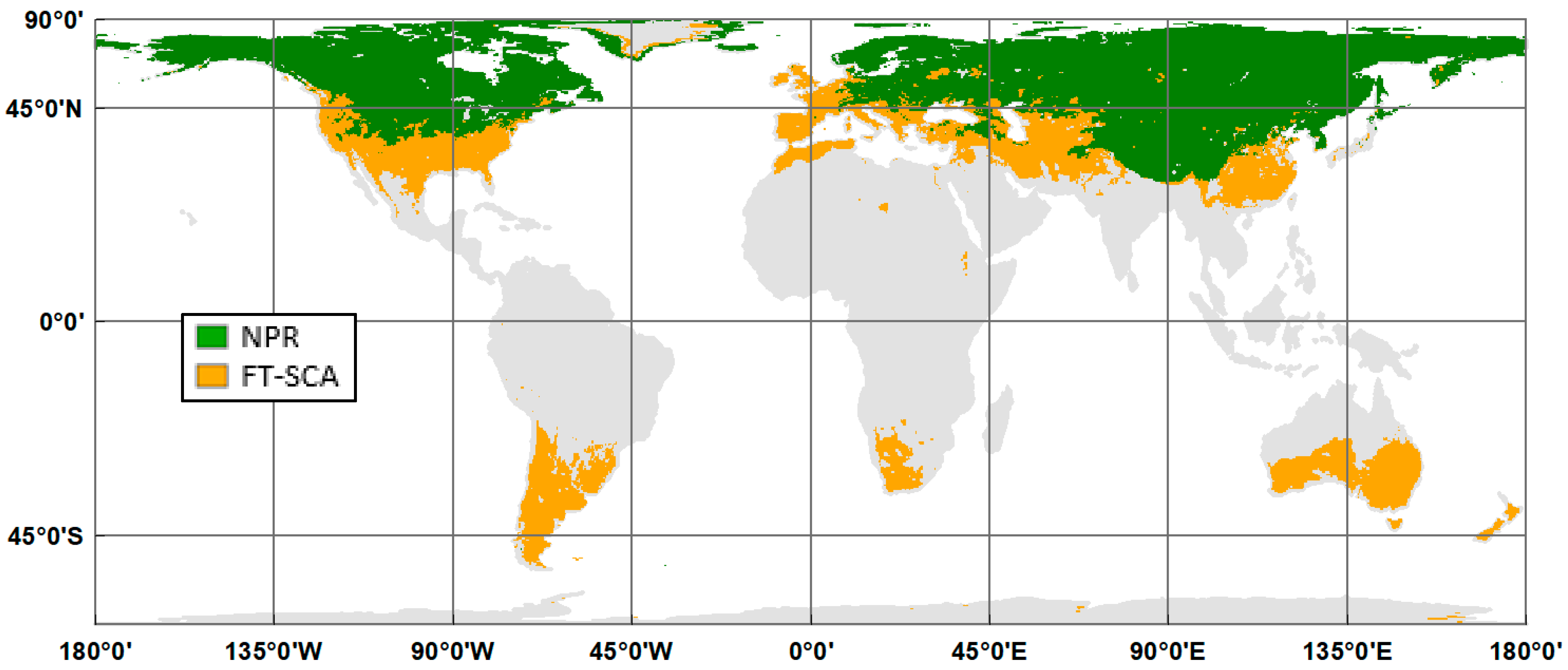
3.1. The SMAP FT Global Data Domain

The SMAP R16 global grid FT products encompass ~51.4% (~73 million km²) of the global land area (Figure 2). The SMAP FT global grid products cover the same area as the heritage FT-ESDR [31], encompassing all land areas where seasonal frozen temperatures are estimated to be a significant constraint on annual ecosystem productivity. The map in Figure 2 shows areas where the NPR and FT-SCV algorithms are applied. The NPR domain (in green) encompasses areas where seasonal frozen and thawed conditions are persistent enough to generate stable NPR reference thresholds and where the FT reference difference is large enough for suitable algorithm performance (NPR > 0.1). The FT-SCV domain encompasses more southerly latitudes where FT conditions are more transient. The NPR and FT-SCV areas encompass 68 and 32 percent of the global FT classification domain, respectively.

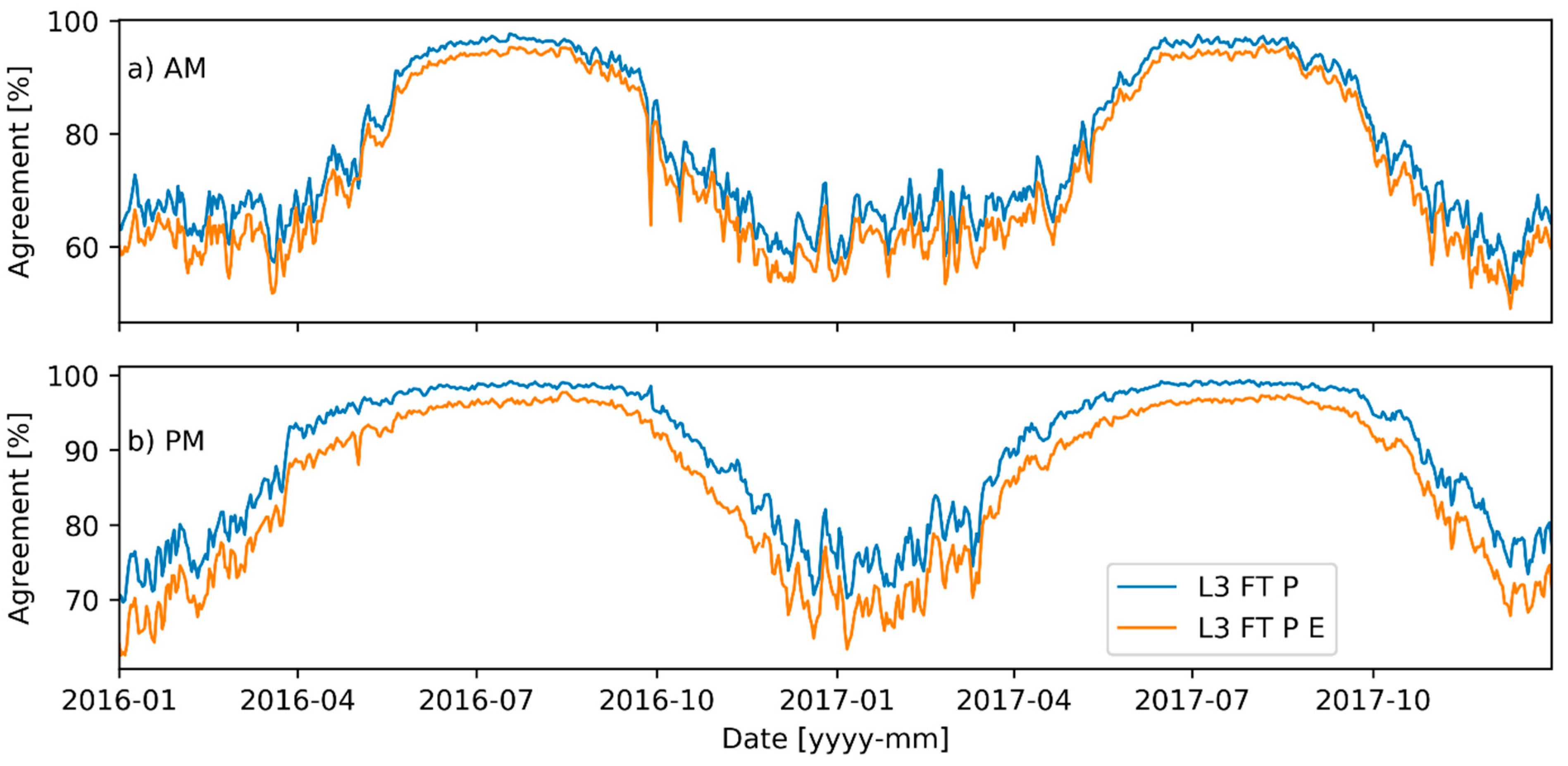
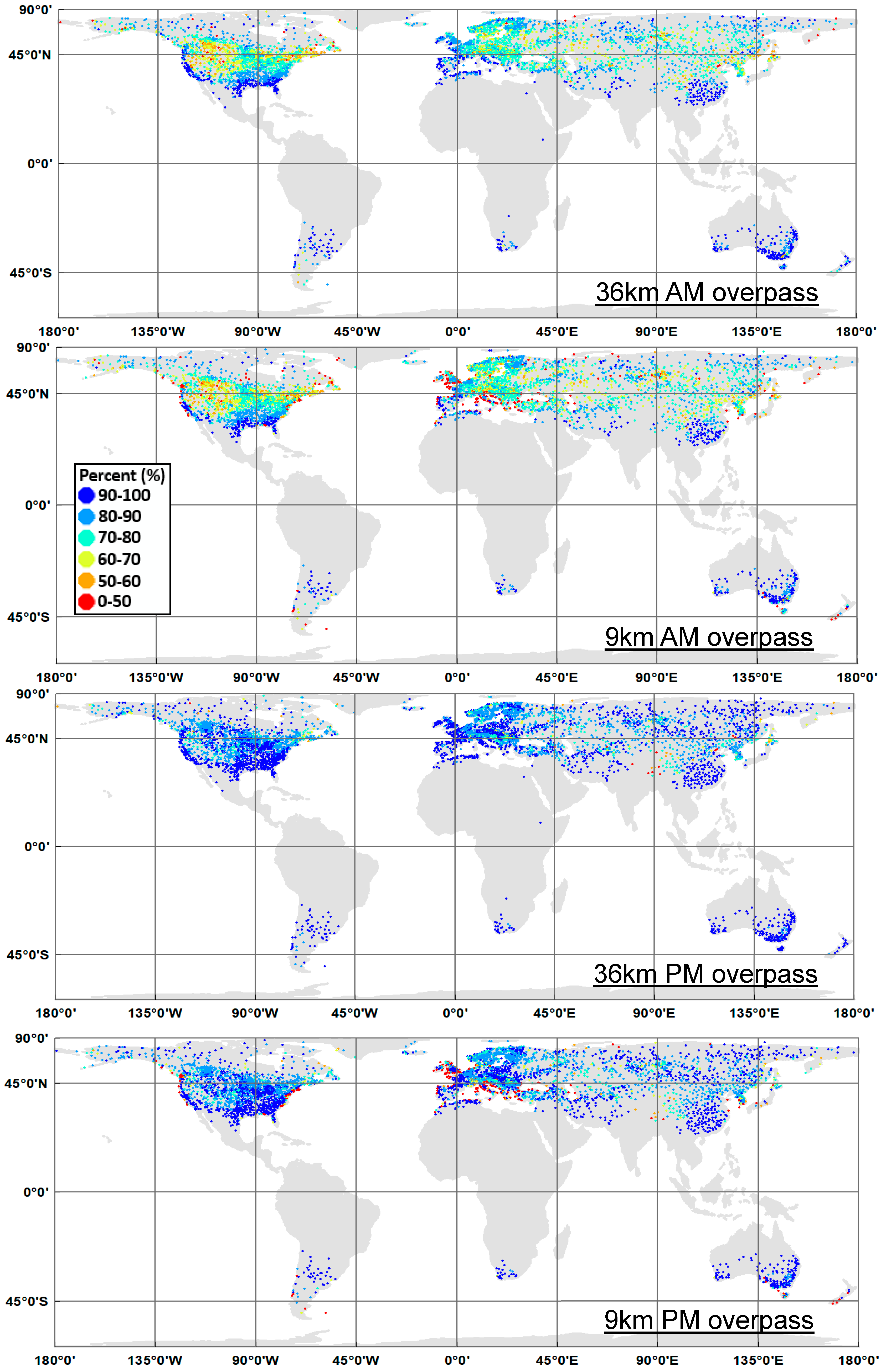
3.2. FT Classification Assessment

A plot of the daily mean AM and PM overpass FT spatial classification accuracies for the global domain from the 9 km and 36 km records is shown in Figure 3. The SMAP FT agreement with the WMO SAT derived FT records is generally higher during the northern hemisphere summer months when the pattern and persistence of non-frozen conditions is more homogeneous and stable. The FT agreement is weaker and more variable during temporally dynamic spring and fall transition periods, and lowest during the northern hemisphere winter months. Lower winter season agreement may be due to uncertainty in the ephemeral FT zone across the southern margin of more stable, seasonally frozen ground. For the 36 km and 9 km products, the PM overpass FT results generally exceed an 80% mean spatial classification accuracy. The AM overpass FT accuracy is somewhat lower than the PM results but is generally above 70%. The lower AM accuracy is consistent with previous FT validation assessments from SMAP and higher frequency satellite microwave sensors [7,11], and may reflect one or more factors, including relatively larger SAT and FT heterogeneity during the morning observations, and a temporal offset between the SMAP 6 AM overpass and the diurnal timing of SAT_min. In addition, the relative FT accuracy differences between satellite AM and PM overpasses may be influenced by remaining unidentified RFI contamination of the Tb retrievals, which may vary between ascending and descending orbits [6]. Varying solar activity [49] may also contribute to differences in the apparent FT bias between satellite overpass times. The validation results over the global domain show relatively small (3–4%) FT accuracy differences between the 9 km and 36 km products, though the apparent accuracy of the 36 km product is higher than the 9 km product for both PM and AM results. Relatively minor differences in FT accuracy between these products may reflect potential noise introduced from the Backus Gilbert Tb interpolation method [50] and the similar effective footprint (~33–40 km) of the two products.

The spatial distribution of mean annual FT accuracy for the 36 km and 9 km products, and AM and PM overpass results in relation to grid cell-to-point comparisons with approximately 5000 global weather stations is shown in Figure 4. The global mean annual FT spatial accuracy of the 36 km product was 78.0 ± 11.5% and 89.6 ± 8.6% for respective AM and PM overpasses from the 2016 record. The FT accuracy pattern for the 2017 record (not shown) was generally consistent and within 1% of the 2016 mean annual FT global accuracy. Lower latitude areas with characteristic warmer temperatures generally show greater mean annual FT accuracy due to a longer non-frozen period. The spatial pattern in FT accuracy also reflects greater Tb signal-to-noise and lower accuracy in forested and mountainous areas. The AM overpass FT accuracy is lower than the PM accuracy, particularly near coastlines and in more transient FT areas. While the spatial pattern in FT accuracy is generally similar between the 9 km and 36 km results, the 36 km accuracy is enhanced when compared to the 9 km product. The SMAP FT accuracy is lower during more heterogeneous seasonal transitions. The SMAP FT-SCV performance is also influenced by uncertainty contributed from the GMAO surface temperatures used for calibrating the algorithm FT threshold. The estimated mean residual error in the GMAO surface temperatures is approximately 1.65 °K and 4.62 °K relative to WMO weather station SAT daily maximum and minimum temperature observations within the FT-SCV domain. This temperature uncertainty contributes approximately 2.0 ± 2.0 to 1.1 ± 2.7 percent of mean daily spatial classification uncertainty to the SMAP FT-SCV results for the satellite PM and AM overpass retrievals, respectively, where the uncertainty is larger during seasonal transition periods.

The overall accuracy from the 36 km and 9 km FT data records is presented in

Table 1. The mean annual FT classification accuracy (%) of SMAP 36 km (L3_FT_P) and 9 km (L3_FT_P_E) daily FT products in relation to surface air temperature-based FT estimates from ~5000 global weather stations. The values in parentheses represent the mean annual FT classification accuracy (%) in the northern (≥45°N) portion of the domain. The FT accuracy is determined from SMAP ascending (PM) and descending (AM) orbital overpass Tb retrievals.

FT Product	AM Overpass	AM Overpass	PM Overpass	PM Overpass
	2016	2017	2016	2017
36 km	78.0 (74.9)	77.8 (74.7)	89.6 (87.8)	89.7 (87.6)
9 km	74.4 (71.8)	74.3 (71.7)	85.6 (84.2)	85.8 (84.0)

. These results summarize the SMAP FT validation assessments against WMO weather station observations for both northern (≥45°N) and global domains over the two-year record. Overall, the PM overpass FT classification results from the 9 km and 36 km products exceed the targeted 80% accuracy threshold for the SMAP baseline mission requirement [8]. The AM FT apparent accuracy is lower than the PM accuracy for both the 36 km and 9 km products, but generally above the 70% targeted accuracy threshold of the minimum mission. The lower FT classification agreement over the northern (≥45°N) domain may be attributed to a larger number of daily FT variations over the annual cycle and to wetter snow conditions during seasonal transitions [7,51], where the L-band snow volume emission becomes significant in the presence of even small amounts of snow liquid water [52]. However, the distribution of other physical landscape factors can degrade the Tb signal-to-noise and influence the associated FT accuracy pattern [51,53].

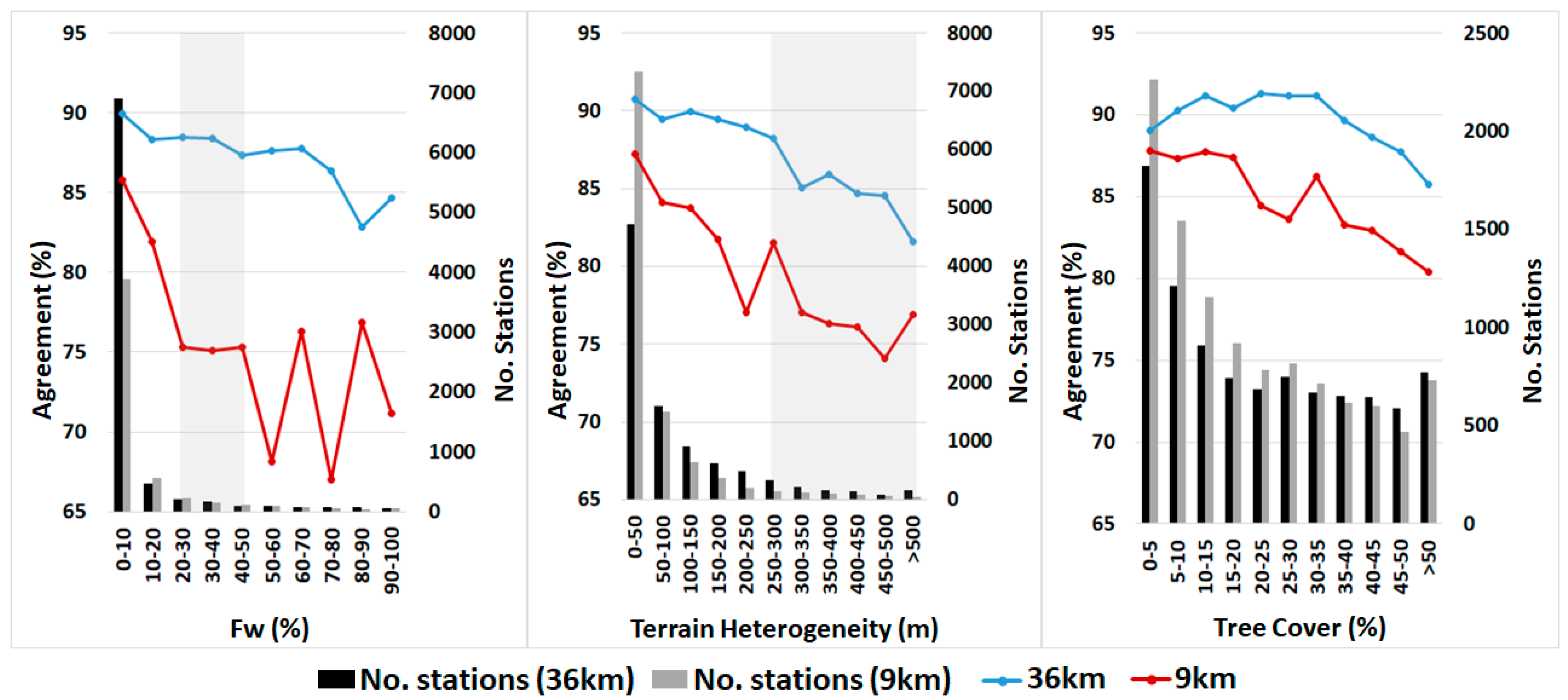
3.3. Landscape Factors Affecting FT Classification Accuracy

The mean annual FT classification agreement was analyzed for the 2016–2017 SMAP PM FT data records from both the 36 km and 9 km global grid products. Generally, we found lower FT accuracy in areas with a higher fw, defined as the spatial proportion of open water within a 36 km and 9 km grid cell derived from the 300 m ESA water body map (Figure 5). The lower FT quality flag was assigned to cells with significant fw (grey shading in Figure 5), while cells with larger (>50%) fw levels, identified from a static water mask (MOD44W), are screened from further processing. The remaining FT cells with fw > 50% are attributed to differences between the ESA and MOD44W water masks, and primarily occur along coastal areas and large water bodies. These water-contaminated grid cells are identified from the ESA water body map used in this study, but were missed by the MOD44W static water map used for water body screening during SMAP operational processing. The inverse relationship between FT accuracy and fw cover is consistent with strong L-band microwave sensitivity to open water, which can degrade the Tb signal from adjacent land areas within the satellite footprint [54,55,56,57]. The FT accuracy was also inversely proportional to the amount of forest cover and terrain complexity within a grid cell, derived from respective MOD44B 250 m vegetation and 30 m DEM data. The mountainous terrain flag was assigned to grid cells with a large (>250 m) elevation spatial standard deviation (SD), identified from the 30 m global DEM (grey shading in Figure 5). The 36 km grid product showed less sensitivity to vegetation cover, terrain heterogeneity and fw constraints than the 9 km grid product. Overall, the combined landscape factors explained approximately 53% and 29% (R², p < 0.01) of the global variation in mean annual FT accuracy from the respective 36 km and 9 km PM products relative to the global SAT station network (Figure 5).

The SMAP FT results are generally sensitive to the predominant frozen or thaw status of the land surface within a coarse (~40-km) radiometer footprint. However, the actual FT pattern may be more spatially complex due to variations in microclimate and land cover conditions that may not be adequately resolved by the satellite footprint [11,40,57]. These factors can contribute to a mismatch between in situ SAT observations that predominantly reflect local land surface conditions and overlapping satellite Tb retrievals representing an integrated regional signal.

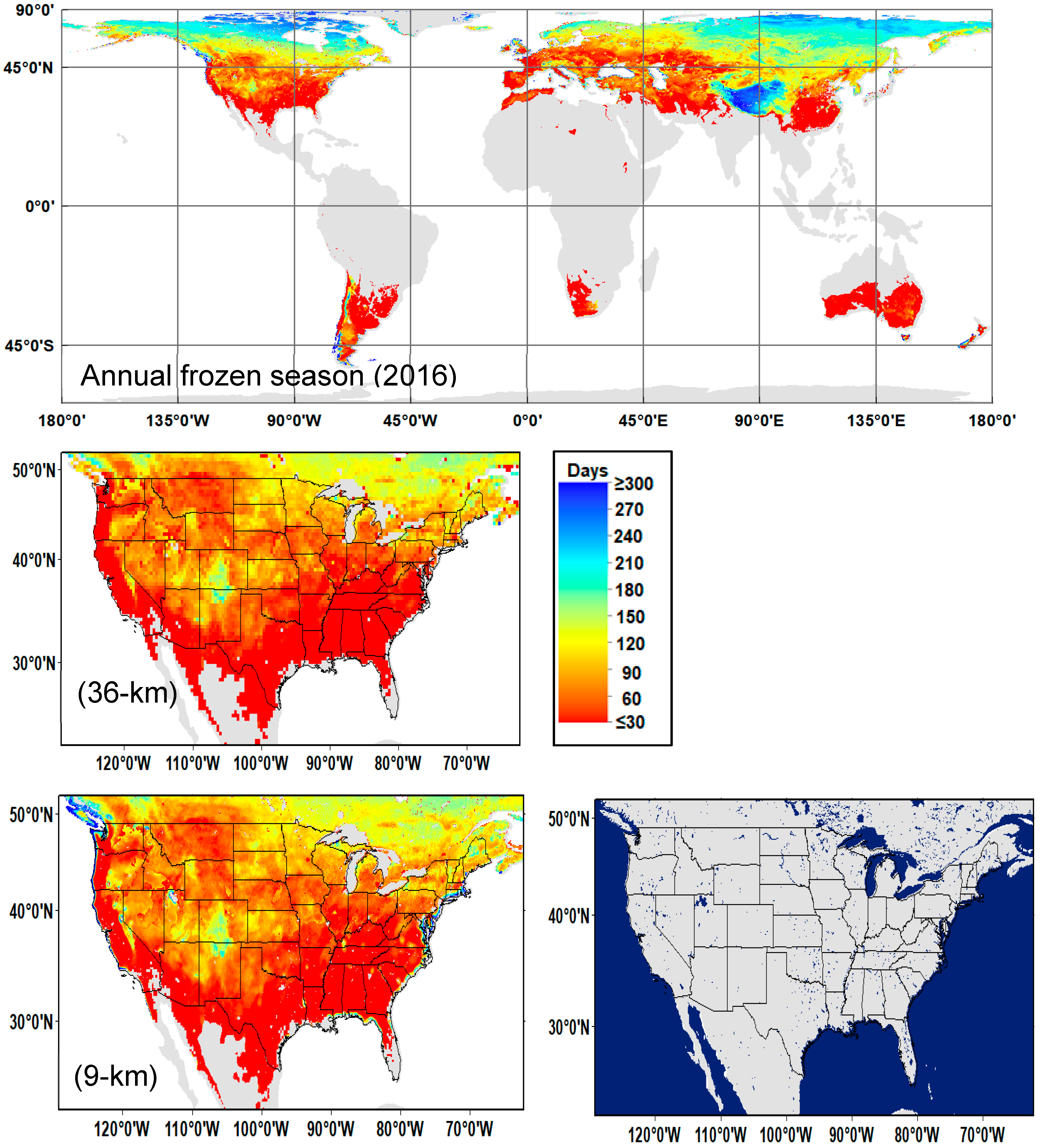
3.4. Spatial Frozen Season Characteristics

The annual frozen season was estimated by summing up the daily FT records for each grid cell, including frozen and transitional conditions, from the 36 km and 9 km grid products. The resulting frozen season map for 2016 from the 9 km grid product is presented (Figure 6), showing a mean frozen season of 112 ± 79 [spatial-SD] days for the global domain. The 2017 frozen season map (not shown) has a consistent global pattern and mean frozen season (112 ± 82 days). The SMAP FT data captures characteristic frozen season increases at higher elevations, including Tibetan Plateau, Andes and Rocky Mountain areas. The frozen season is generally shorter along coastal margins relative to inland areas, which is consistent with more moderate maritime climate conditions in the coastal zone.

The regional depictions of the 2016 annual frozen season over the continental United States are also presented (Figure 6), highlighting differences between the 36 km and 9 km FT products. The SMAP 9 km grid FT data shows a general enhancement of the frozen season pattern relative to the 36 km product. The mean and spatial SD of the frozen season distributions are 57 ± 33 and 62 ± 42 days for respective 36 km and 9 km products. The relatively large SD is associated with the wide distribution of annual frozen days over the continental US, ranging from relatively few (<9) frozen days across the warmer southern states to a much longer frozen season in the northeastern states and in higher elevation mountain areas (Figure 6). In addition, the relatively large variation in the frozen season may be associated with heterogeneous radiometric properties of the land surface in neighboring grid cells and within the satellite footprint during FT transitions. The larger SD in the 9 km product reflects the fact that greater frozen season heterogeneity was represented, including improved delineation of characteristic elevation and regional climate-driven patterns over the intermountain west. The larger SD in the 9 km product also reflects an anomalous frozen season increase along coastal boundaries and large inland water bodies (inset map in Figure 6) that is greatly reduced in the 36 km product. The larger frozen season along coastal boundaries is attributed to water contamination of the adjacent Tb retrievals over land, which may be exacerbated by the BG interpolation used in the 9 km product. The associated water contamination accounts for the much stronger FT accuracy decline in the 9 km product in areas with higher fw levels relative to the 36 km product (Figure 5). However, the L3_FT products assign a lower quality flag to grid cells with fw levels ranging from 20–50% cover from an ancillary static (MOD44W) water mask, while a majority of grid cells with higher fw levels are excluded from the FT processing.

3.5. Regional Case Studies

The potential utility of the SMAP FT products was evaluated from two regional case studies highlighting selected science applications indicated in prior studies (e.g., [4,58,59]). The first case study applies the SMAP NPR algorithm portion of the FT record to determine the primary spring thaw timing over Alaska and its relationship to the growing season onset and seasonal increase in vegetation gross primary production (GPP), represented by the SMAP Level 4 Carbon product [37]. The second case study highlights the FT-SCV portion of the domain for detecting transient frost events in Australia, which can be damaging to cropland and natural vegetation [59,60].

3.5.1. Spring Onset Characteristics over Alaska

The spring onset is closely linked with seasonal thaw timing and the initiation of the vegetation growing season, where the frozen season is a significant constraint on annual vegetation growth [61]. The primary spring thaw date was determined from the 9 km SMAP daily global FT record over Alaska as the first date (DOY) for which 12 out of 15 successive days from March to July are classified as non-frozen for each year of record [1]. The growing season onset was also determined for each grid cell and study year as the mean DOY when GPP was between 10% and 20% of the annual maximum daily rate (GPP_max, [4]). Here, daily GPP over Alaska was obtained for the study period from the SMAP L4_C global product [62], where GPP and other carbon flux variables are derived using a satellite-driven terrestrial carbon model informed by MODIS vegetation and SMAP assimilation enhanced surface-to-root zone soil moisture and temperature inputs [37]. The SMAP L4_C product is produced in the same 9 km global grid format as the L3_FT_E global product.

The resulting pattern of spring thaw timing and growing season onset from the SMAP record is shown in Figure 7. The 2016 record was associated with a major El Niňo and showed generally earlier thaw timing over Alaska, which is consistent with above-normal spring temperatures relative to 2017 [63,64]. However, the spatial pattern of thaw timing was similar for both years, beginning in mid-March over southwest Alaska and progressing into mid-May at higher latitudes and elevations.

The growing season onset indicated by the SMAP L4_C GPP record lagged the primary thaw timing by approximately 46 ± 24 (spatial SD) days over Alaska (Figure 7). The SMAP FT record indicates generally earlier spring thaw timing than the FT retrievals from higher frequency (~37 GHz) Tb measurements [4,65]. These results, which are consistent with earlier studies, indicate that the SMAP L-band FT record may be more sensitive to initial surface thawing and wet snow conditions within a deeper snow layer, relative to higher frequency retrievals that are sensitive to more ephemeral surface FT variations [9,24,66]. The seasonal progression in the proportional area of non-frozen conditions preceded the spring GPP growing season onset in Alaska for both study years. The timing and rate of increase in thawed area for each year was also inversely proportional to spring productivity, whereby cumulative daily GPP showed higher productivity in 2016 due to earlier spring thaw than in 2017 (Figure 7). These results confirm the importance of the spring FT signal as an effective proxy for the seasonal release of frozen temperature constraints on ecosystem productivity and terrestrial carbon (CO₂) sink activity in the boreal-Arctic [4,61], while the SMAP L-band signal is expected to have greater sensitivity to soil FT conditions relative to higher frequency Tb based FT records [1].

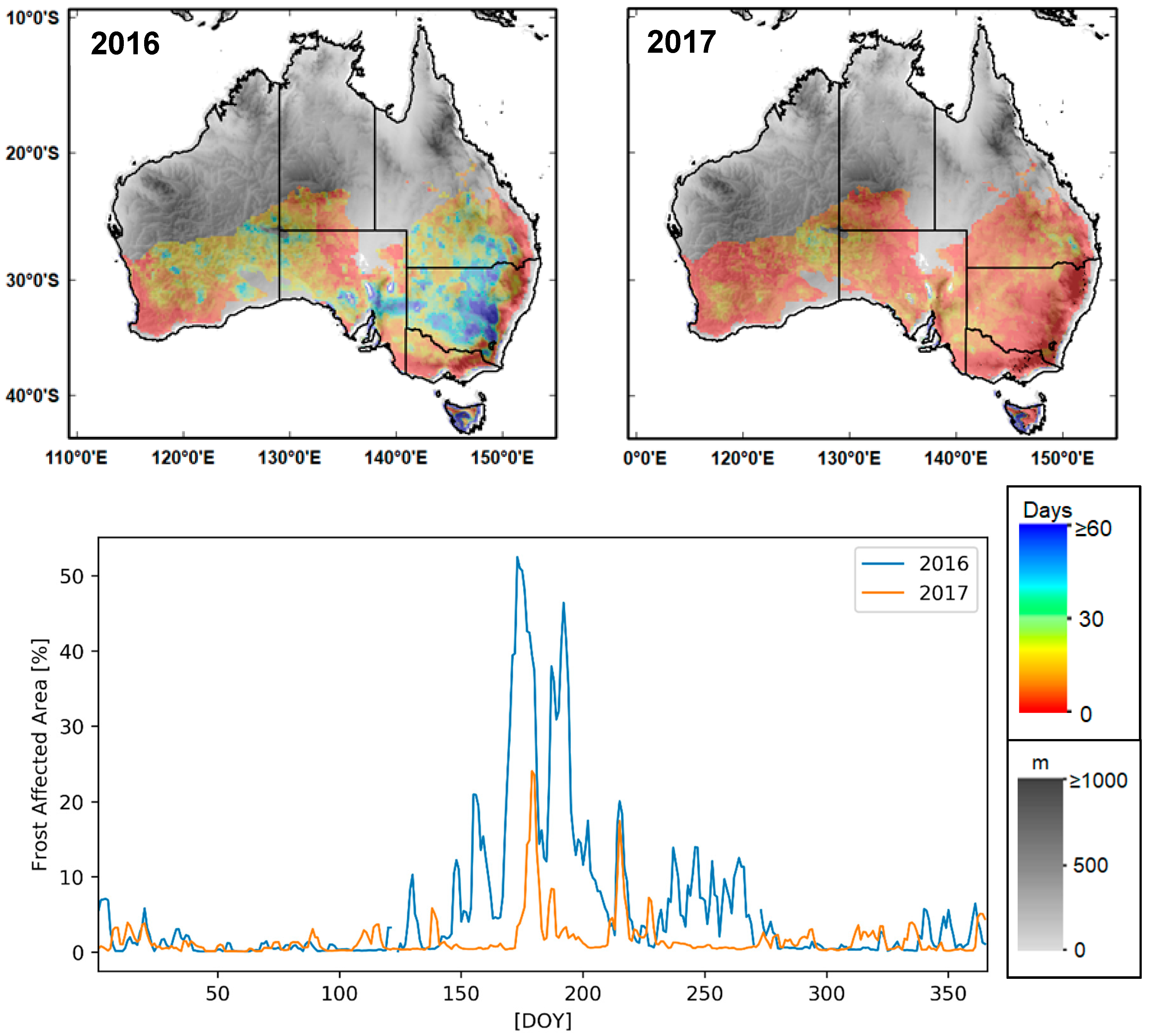
3.5.2. Australian Frost Events

Recent studies have reported that the frequency of annual frost events has increased across southern Australia [67,68]. Southern Australia has a characteristic temperate climate with little contrast between mean summer and winter temperatures, which may lead to fewer cold weather adaptations and greater vegetation susceptibility to potentially damaging frost. Frost occurrence in the region has resulted in significant agricultural crop damage and productivity losses [60,69], while the wheat belt of southwest Australia experienced unusual frost events before harvest in September 2016 [70].

The SMAP 9 km global daily FT records were analyzed over Australia to evaluate the spatial and seasonal pattern of frost occurrence over the region in 2016 and 2017. Here, frost occurrence represented days with classified frozen or transitional (AM or PM) FT conditions [59]. The seasonal pattern of frost-affected areas over the Australian portion of the global L3_FT domain is shown for each year of record in Figure 8. The SMAP-derived frost distribution in both years is consistent with the annual frost potential pattern established from long-term surface air temperature measurements using a standard 2 °C FT threshold [68,71,72]. Frost occurrence is primarily the result of nighttime freezing followed by subsequent daytime thawing, indicated by the transitional (AM frozen, PM thaw) FT condition from the SMAP FT daily composite. However, the SMAP results indicate a larger number of frost events in 2016 than in 2017. These results contrast with regional weather station observations that indicate frequent nighttime frosts across southern Australia from June to September 2017 [73], but warmer-than-normal air temperatures and lower documented frost occurrence in 2016 [74]. The apparent discrepancy may be attributed to annual climate variability and differences in physical sensing depth between the SMAP L-band FT retrievals representing surface soil and snow cover (when present) conditions, and a weather station frost condition defined from overlying daily minimum air temperatures. In 2016, Australia had above-average rainfall associated with a strong El Niňo, whereas the rainfall in 2017 was below normal. Generally, drier soil conditions may account for fewer detected SMAP FT frost events in 2017, owing to the degraded FT dielectric contrast at low soil moisture levels [75]. Despite generally dry conditions, a succession of cold fronts and cold polar air intrusions from June to August resulted in significant snowfall across higher elevation areas in southeastern Australia in 2017 [76,77]. The insulating effect of snow cover provides a strong thermal buffer between SAT extremes, including ephemeral frost events, and more stable underlying snow and soil layers [7,78]; this may also account for the lower number of SMAP FT-derived frost days in 2017 over the mountain areas of southeast Australia relative to SAT-derived frost events reported from the regional weather station network. Therefore, relatively warmer and drier climate areas may promote a lower frost classification accuracy in relation to in situ SAT observations.

4. Discussion and Conclusions

The latest (R16) SMAP FT records are derived using combined NPR and FT-SCV retrieval algorithms, and extend over a larger global domain than prior product releases. The SMAP global FT products include the mitigation of suspected false freeze and thaw retrievals identified in earlier product releases. The FT accuracy was assessed using in situ daily surface air temperature measurements from approximately 5000 weather stations located across the global domain. Our results indicate that the PM overpass FT results from the 9 km and 36 km products exceed the targeted 80% accuracy threshold for the SMAP baseline mission requirement [8]. The AM FT accuracy is significantly lower than the PM FT results for both the 36 km and 9 km products, but generally exceeds the 70% accuracy threshold of the minimum mission requirement. The FT accuracy is generally greater during the northern hemisphere summer, and is lower in winter and during seasonal transitions when landscape heterogeneity in snow cover and microclimate conditions is enhanced relative to the coarse (~40 km) L-band radiometer footprint.

A key assumption of the NPR and FT-SCV algorithms is that major temporal shifts in the SMAP Tb record are caused by the characteristic large landscape dielectric changes that occur during FT transitions, rather than by other potential factors including large precipitation events or changes in surface inundation, snow cover or canopy biomass. The physical basis for the NPR algorithm requires relatively stable freeze and thaw seasonal reference conditions and enough difference between NPR reference states to establish a suitable signal-to-noise ratio for the FT classification. These criteria limit the area where the NPR algorithm can be applied. Based on the three-year SMAP data analysis, the NPR reference difference needed to be larger than 0.1 in order to enable reliable FT results. On the other hand, the FT-SCV algorithm exploits the large characteristic dielectric and associated Tbv shift between predominantly frozen and non-frozen conditions, influenced by the correlation between the L-band Tbv and physical temperature. Favorable correlation (|R| > 0.5) between Tbv and surface temperature (represented from the GMAO reanalysis) is a requirement for the FT-SCV application, while the associated Tbv and temperature relationship is used to define the Tbv FT threshold for each grid cell in the FT-SCV algorithm. Nevertheless, there are some grid cells where both algorithms can be applied, though these areas represent a relatively small (<10%) portion of the SMAP FT global domain. In these areas, the NPR is selected over the FT-SCV during operational processing because the NPR is consistent with the primary baseline algorithm established from the initial SMAP FT science algorithm and product release [7]. This approach helps to preserve product self-consistency.

The SMAP FT retrieval patterns showed no apparent artifacts between the NPR and FT-SCV domains. The FT metrics were generally consistent between NPR and FT-SCV derived results despite the different areas and conditions represented by the two algorithms. The SMAP global FT accuracy is influenced by landscape heterogeneity within the sensor footprint and was degraded in areas with higher fw cover, terrain variability, and vegetation cover. Together, these landscape factors accounted for approximately 29–53% of the global variability in mean annual FT classification accuracy from respective 36 km and 9 km PM products relative to the global SAT weather station network (Figure 5). Regions influenced by the landscape factors largely represent heterogeneous grid cells encompassing mountainous regions, coastal areas, dense forests and large open water bodies. The negative impacts from large open water bodies (20–50% fw), active precipitation, and complex terrain are partially represented by the product data quality (QA) flags. Excluding these low QA flagged grid cells resulted in FT accuracy improvements of up to 2.73% for the 9 km FT product, but less than 1% improvement in the 36 km product. Other potential negative impacts from known RFI, excessive open water (fw > 50%) and permanent ice/snow cover are identified from ancillary information and are masked prior to the FT retrievals during SMAP operational processing. However, our results also indicate the important role of vegetation cover affecting FT accuracy, which is neglected in the current QA flagging process. The current screening process also misses a significant number (~181 ± 32) of excessive water contaminated grid cells having relatively low FT accuracy (Figure 5); these areas are represented in the ESA water body map used in this study, but are missing from the static water map (MOD44W) used for SMAP operational processing. Other potential factors influencing FT accuracy include the correlation (R) between SMAP Tb retrievals and GMAO surface temperatures used for the FT-SCV calibration (Figure 1), and the seasonal difference between NPR frozen and non-frozen reference conditions. These additional constraints represent potential candidates for future QA enhancements.

Potential noise introduced from the BG Tb interpolation used for the L3_FT_P_E retrievals, and an effective spatial resolution closer to 33 km, may also contribute to a lower-than-expected performance in this product relative to the L3_FT_P standard 36 km product. However, the validation results showed relatively small (3–4%) FT accuracy differences between both products; these accuracy differences were further reduced (~1.5%) by excluding low quality flagged grid cells. Although the overall FT accuracy of the 36 km product was slightly better than that of the 9 km product for both the PM and AM results, the finer grid product showed generally enhanced delineation of FT spatial patterns (e.g., Figure 6).

The science utility of the SMAP FT products was highlighted for two regional case studies involving spring onset variability in Alaska and frost occurrence over Australia. Our results confirm the ecological significance of the FT retrieval, including the seasonal thaw and spring onset, and anomalous frost detection, in assessing FT impacts on vegetation productivity. However, our results also reveal critical differences in the SMAP L-band FT sensitivity, including an early spring thaw pattern that occurs approximately 6.6 ± 3.4 weeks prior to growing season onset, and frost events that more closely resemble soil rather than surface air temperature conditions. These results contrast with similar studies using higher frequency satellite Tb retrievals [4,59] and may reflect a greater SMAP L-band FT sensitivity to snow and soil properties. The relatively high mean annual FT classification accuracy reported in warmer climate areas may mask FT uncertainty because the intermittent frost events in these areas represent only a small part of the annual cycle.

Although the SMAP L-band Tb retrievals are expected to have enhanced sensitivity to surface soil FT conditions under low to moderate vegetation cover, the SMAP FT algorithms and retrievals characterize the predominant frozen or non-frozen condition within a grid cell and do not distinguish different landscape elements within the sensor footprint. The finer 9 km grid product provides a level of FT spatial enhancement contributed from the BG optimal Tb interpolation, which offers potential benefits for delineating regional climate variability. However, the associated data quality flags should be used in evaluating the level of confidence in the FT results, because the 9 km product shows a visibly stronger performance decline with increasing landscape heterogeneity relative to the 36 km grid product. Further improvements to the L1C_B_E product may include mitigation of surface water contamination in the Tb retrievals over adjacent land areas and alternative Tb interpolation approaches such as rSIR [79] or machine learning; these refinements are expected to propagate to better accuracy and performance in the 9 km grid FT product.

The latest (R16) version of the SMAP L3_FT products examined in this study covers more than half of the global land area, including all areas where the frozen temperatures are a key limitation to annual ecosystem productivity. However, future products may include a larger domain covering all snow/ice affected regions (e.g., Greenland and Antarctica). A potential future product enhancement may also include FT retrievals from both FT-SCV and NPR algorithms, where conditions are suitable for their joint application. Enhanced delineation of different landscape FT components, including soil, snow cover and vegetation, may allow for an improved understanding of FT related controls on terrestrial carbon, water and energy cycles, and their interactions. Vegetation optical depth (VOD) information from SMOS could help to improve the delineation of landscape FT components and/or vegetation biomass effects on NPR derived FT sensitivity. Potentially complimentary information from other satellite observations, including higher frequency Tb retrievals from AMSR2 and C-band (In)SAR from Sentinel-1, may also provide complimentary information to improve SMAP Tb and FT spatial enhancements and the delineation of landscape FT elements. Future L3_FT products may include these algorithms and product enhancements while also benefitting from ongoing Tb calibration refinements enabled through a longer data record.

References

1. Kim, Y.; Kimball, J.S.; Zhang, K.; McDonald, K.C. Satellite detection of increasing Northern Hemisphere non-frozen seasons from 1979 to 2008: Implications for regional vegetation growth. Remote Sens. Environ. 2012, 121, 472–487. [Google Scholar] [CrossRef]
2. Xu, X.; Derksen, C.; Yueh, S.H.; Dunbar, R.S.; Colliander, A. Freeze/thaw detection and validation using Aquarius’ L-band backscattering data. IEEE J. Sel. Top. Appl. Earth Obs. Remote Sens. 2016, 9, 1370–1381. [Google Scholar] [CrossRef]
3. Zhang, K.; Kimball, J.S.; Kim, Y.; McDonald, K.C. Changing freeze-thaw seasons in northern high latitudes and associated influences on evapotranspiration. Hydrol. Process. 2011, 25, 4142–4151. [Google Scholar] [CrossRef] [Green Version]
4. Parazoo, N.C.; Arneth, A.; Pugh, T.A.M.; Smith, B.; Steiner, N.; Luus, K.; Commance, R.; Benmergui, J.; Stofferahn, E.; Liu, J.; et al. Spring photosynthetic onset and net CO2 uptake in Alaska triggered by landscape thawing. Glob. Chang. Biol. 2018, 24, 3416–3435. [Google Scholar] [CrossRef] [PubMed]
5. Park, H.; Kim, Y.; Kimball, J.S. Widespread permafrost vulnerability and soil active layer increases over the high northern latitudes inferred from satellite remote sensing and process model assessments. Remote Sens. Environ. 2016, 175, 349–358. [Google Scholar] [CrossRef]
6. Rautiainen, K.; Parkkinen, T.; Lemmetyinen, J.; Schwank, M.; Wiesman, A.; Ikonen, J.; Derksen, C.; Davydov, S.; Davydova, A.; Bioke, J.; et al. SMOS prototype algorithm for detecting autumn soil freezing. Remote Sens. Environ. 2016, 180, 346–360. [Google Scholar] [CrossRef]
7. Derksen, C.; Xu, X.; Dunbar, R.S.; Colliander, A.; Kim, Y.; Kimball, J.S.; Black, T.A.; Euskirchen, E.; Langlois, A.; Loranty, M.M.; et al. Retrieving landscape freeze/thaw state from Soil Moisture Active Passive (SMAP) radar and radiometer measurements. Remote Sens. Environ. 2017, 194, 48–62. [Google Scholar] [CrossRef]
8. Entekhabi, D.; Njoku, E.G.; Neill, P.E.O.; Kellogg, K.H.; Crow, W.T.; Edelstein, W.N.; Entin, J.K.; Goodman, S.D.; Jackson, T.; Johnson, J.; et al. The Soil Moisture Active and Passive (SMAP) mission. Proc. IEEE 2010, 98, 704–716. [Google Scholar] [CrossRef]
9. Roy, A.; Toose, P.; Williamson, M.; Rowlandson, T.; Derksen, C.; Royer, A.; Berg, A.A.; Lemmetyinen, J.; Arnold, L. Response of L-band brightness temperatures to freeze/thaw and snow dynamics in a prairie environment from ground-based radiometer measurements. Remote Sens. Environ. 2017, 191, 67–80. [Google Scholar] [CrossRef]
10. Chaubell, M.J.; Chan, S.; Dunbar, R.S.; Peng, J.; Yueh, S. SMAP Enhanced L1C Radiometer Half-Orbit 9 km EASE-Grid Brightness Temperatures, Version 2; NASA National Snow and Ice Data Center Distributed Active Archive Center: Boulder, CO, USA, 2018. [CrossRef]
11. Kim, Y.; Kimball, J.S.; Glassy, J.; Du, J. An extended global Earth system data record on daily landscape freeze-thaw status determined from satellite passive microwave remote sensing. Earth Syst. Sci. Data 2017, 9, 133–147. [Google Scholar] [CrossRef]
12. Kerr, Y.; Waldteufel, P.; Richaume, P.; Wigneron, J.; Ferrazzoli, P.; Mahmoodi, A.; al Bitar, A.; Cabot, F.; Gruhier, C.; Juglea, S.; et al. The SMOS soil moisture retrieval algorithm. IEEE Trans. Geosci. Remote 2012, 50, 1384–1403. [Google Scholar] [CrossRef]
13. Rowlandson, T.L.; Berg, A.A.; Roy, A.; Kim, E.; Lara, R.P.; Powers, J.; Lewis, K.; Houser, P.; McDonald, K.; Toose, P.; et al. Capturing agricultural soil freeze/thaw state through remote sensing and ground observations: A soil freeze/thaw validation campaign. Remote Sens. Environ. 2018, 211, 59–70. [Google Scholar] [CrossRef]
14. Wigneron, J.-P.; Jackson, T.J.; O’Neill, P.; Lannoy, D.; de Rosnay, P.; Walker, J.P.; Ferrazzoli, P.; Mironov, V.; Bircher, S.; Grant, J.P.; et al. Modelling the passive microwave signature from land surfaces: A review of recent results and application to the L-band SMOS and SMAP soil moisture retrieval algorithms. Remote Sens. Environ. 2017, 192, 238–262. [Google Scholar] [CrossRef]
15. Podest, E.; McDonald, K.C.; Kimball, J.S. Multisensor microwave sensitivity to freeze/thaw dynamics across a complex boreal landscape. IEEE Trans. Geosci. Remote 2014, 52, 6818–6828. [Google Scholar] [CrossRef]
16. Xu, X.; Dunbar, R.S.; Derksen, C.; Colliander, A.; Kim, Y.; Kimball, J.S. SMAP Enhanced L3 Radiometer Global and Northern Hemisphere Daily 9 km EASE-Grid Freeze/Thaw State, Version 2; NASA National Snow and Ice Data Center Distributed Active Archive Center: Boulder, CO, USA, 2018. [CrossRef]
17. Xu, X.; Dunbar, R.S.; Derksen, C.; Colliander, A.; Kim, Y.; Kimball, J.S. SMAP L3 Radiometer Global and Northern Hemisphere Daily 36 km EASE-Grid Freeze/Thaw State, Version 2; NASA National Snow and Ice Data Center Distributed Active Archive Center: Boulder, CO, USA, 2018. [CrossRef]
18. Kraatz, S.; Jacobs, J.M.; Schroeder, R.; Cho, E.; Cosh, M.; Seyfried, M.; Prueger, J.; Livingston, S. Evaluation of SMAP Freeze/thaw retrieval accuracy at Core Validation Sites in the Continuous United States. Remote Sens. 2018, 10, 1483. [Google Scholar] [CrossRef]
19. Wang, P.; Zhao, T.; Shi, J.; Hu, T.; Roy, A.; Qui, Y.; Lu, H. Parameterization of the freeze/thaw discriminant function algorithm using dense in-situ observation network data. Int. J. Digit. Earth 2018, 11. [Google Scholar] [CrossRef]
20. Chan, S. SMAP L1C Radiometer Half-Orbit 36 km EASE-Grid Brightness Temperatures, Version 4; NASA National Snow and Ice Data Center Distributed Active Archive Center: Boulder, CO, USA, 2018. [CrossRef]
21. Piepmeier, J.R.; Focardi, P.; Horgan, K.A.; Knuble, J.; Ehsan, N.; Lucey, J.; Brambora, C.; Brown, P.R.; Hoffman, P.J.; French, R.T.; et al. SMAP L-band Microwave Radiometer: Instrument Design and First Year on Orbit. IEEE Trans. Geosci. Remote Sens. 2017, 55, 1954–1966. [Google Scholar] [CrossRef]
22. Poe, G. Optimum interpolation of imaging microwave radiometer data. IEEE Trans. Geosci. Remote Sens. 1990, 28, 800–810. [Google Scholar] [CrossRef] [Green Version]
23. Colliander, A.; Jackson, T.J.; Chan, S.K.; O’Neill, P.; Bindlish, R.; Cosh, M.H.; Caldwell, T.; Walker, J.P.; Berg, A.; McNaim, H.; et al. An assessment of the differences between spatial resolution and grid size for the SMAP enhanced soil moisture product over homogeneous sites. Remote Sens. Environ. 2018, 207, 65–70. [Google Scholar] [CrossRef]
24. Rautiainen, K.; Lemmetyinen, J.; Schwank, M.; Kontu, A.; Ménard, C.; Mätzler, C.; Drusch, M.; Wiesmann, A.; Ikonen, J.; Pulliainen, J. Detection of soil freezing from L-band passive microwave observations. Remote Sens. Environ. 2014, 147, 206–218. [Google Scholar] [CrossRef]
25. Roy, A.; Royer, A.; Derksen, C.; Brucker, L.; Langlois, A.; Mialon, A.; Kerr, Y. Evaluation of spaceborne L-band radiometer measurements for terrestrial freeze/thaw retrievals in Canada. J. Sel. Top. Appl. Earth Obs. Remote Sens. 2015, 8, 4442–4459. [Google Scholar] [CrossRef]
26. Du, J.; Kimball, J.S.; Moghaddam, M. Theoretical Modeling and Analysis of L- and P-band radar backscatter sensitivity to soil active layer dielectric variations. Remote Sens. 2015, 7, 9450–9472. [Google Scholar] [CrossRef]
27. Wigneron, J.P.; Chanzy, A.; Calvet, J.C.; Bruguier, N. A simple algorithm to retrieve soil moisture and vegetation biomass using passive microwave measurements over crop fields. Remote Sens. Environ. 1995, 51, 331–341. [Google Scholar] [CrossRef]
28. Kim, Y.; Kimball, J.S.; Glassy, J.; McDonald, K.C. MEaSUREs Global Record of Daily Landscape Freeze/Thaw Status, Version 4; NASA National Snow and Ice Data Center Distributed Active Archive Center: Boulder, CO, USA, 2017. [CrossRef]
29. Ulaby, F.T.; Long, D.G.; Blackwell, W.J.; Elachi, C.; Fung, A.K.; Ruf, C.; Sarabandi, K.; Zebker, H.A.; Van Zyl, J. Microwave Radar and Radiometric Remote Sensing; University of Michigan Press: Ann Arbor, MI, USA, 2014. [Google Scholar]
30. Zhang, L.; Shi, J.; Zhang, Z.; Zhao, K. The estimation of dielectric constant of frozen soil-water mixture at microwave bands. In Proceedings of the IEEE International Geoscience and Remote Sensing Symposium (IGARSS), Melbourne, Australia, 21–26 July 2013; Volume 4, pp. 2903–2905, IEEE Cat. No. 03CH37477. [Google Scholar]
31. Kim, Y.; Kimball, J.S.; McDonald, K.C.; Glassy, J. Developing a global data record of daily landscape freeze/thaw status using satellite passive microwave remote sensing. IEEE Trans. Geosci. Remote Sens. 2011, 49, 949–960. [Google Scholar] [CrossRef]
32. Leduc-Leballeur, M.; Picard, G.; Macelloni, G.; Arnaud, L.; Brogioni, M.; Mialon, A.; Kerr, Y.H. Influence of snow surface properties on L-band brightness temperature at Dome C, Antarctica. Remote Sens. Environ. 2017, 199, 427–436. [Google Scholar] [CrossRef]
33. Schwank, M.; Rautiainen, K.; Matzler, C.; Stahli, M.; Lemmetyinen, J.; Pulliainen, J.; Vehvilainen, J.; Kontu, A.; Ikonen, J.; Menard, C.B.; et al. Model for microwave emission of a now-covered ground with focus on L band. Remote Sens. Environ. 2014, 154, 180–191. [Google Scholar] [CrossRef]
34. O’Neill, P.E.; Chan, S.; Njoku, E.G.; Jackson, T.; Bindlish, R. SMAP Enhanced L3 Radiometer Global Daily 9 km EASE-Grid Soil Moisture, Version 2; NASA National Snow and Ice Data Center Distributed Active Archive Center: Boulder, CO, USA, 2018. [CrossRef]
35. O’Neill, P.E.; Chan, S.; Njoku, E.G.; Jackson, T.; Bindlish, R. SMAP Enhanced L3 Radiometer Global Daily 36 km EASE-Grid Soil Moisture, Version 5; NASA National Snow and Ice Data Center Distributed Active Archive Center: Boulder, CO, USA, 2018. [CrossRef]
36. Reichle, R.H. The MERRA-Land data product. GMAO Office Note 3 (Version 1.2); GMAO Office: Greenbelt, MD, USA, 2012; p. 38. Available online: http://gmao.gsfc.nasa.gov/pubs/docs/Reichle541.pdf (accessed on 21 December 2018).
37. Jones, A.L.; Kimball, S.J.; Reichle, H.R.; Madani, N.; Glassy, J.; Ardizzone, V.J.; Colliander, A.; Cleverly, J.; Desai, R.A.; Eamus, D.; et al. The SMAP Level 4 Carbon Product for Monitoring Ecosystem Land-Atmosphere CO2 exchange. IEEE Trans. Geosci. Remote Sens. 2017, 55, 6517–6532. [Google Scholar] [CrossRef]
38. Chew, C.; Lowe, S.; Parazoo, N.; Esterhuizen, S.; Oveisgharan, S.; Podest, E.; Zuffada, C.; Freedman, A. SMAP radar receiver measures land surface freeze/thaw state through capture of forward-scattered L-band signals. Remote Sens. Environ. 2017, 198, 333–344. [Google Scholar] [CrossRef]
39. National Weather Services (NWS): Surface Observations, Federal Meteorological Handbook no 1 (FCM-H1–1988); Department of Commerce, Office Federal Coordinator: Washington, DC, USA, 1988.
40. Du, J.; Kimball, J.S.; Azarderakhsh, M.; Dunbar, R.S.; Moghaddam, M.; McDonald, K.C. Classification of Alaska Spring Thaw Characteristics using satellite L-band Radar Remote Sensing. IEEE Trans. Geosci. Remote Sens. 2015, 53, 542–556. [Google Scholar]
41. Du, J.; Kimball, J.S.; Galantowicz, J.; Kim, S.; Chan, S.K.; Reichle, R.; Jones, L.A.; Watts, J.D. Assessing global surface water inundation dynamics using combined satellite information from SMAP, AMSR2 and Landsat. Remote Sens. Environ. 2018, 213, 1–17. [Google Scholar] [CrossRef] [PubMed]
42. Defourney, P.; Kirches, G.; Brockmann, C.; Boettcher, M.; Peters, M.; Bontemps, S.; Lamarche, C.; Schlerf, M.; Santoro, M. Land Cover CCI: Product User Guide Version 2; ESA Public Document CCI-LC-PUG: Belgium, 2016; Available online: http://maps.elie.ucl.ac.be/CCI/viewer/download/ESACCI-LC-PUG-v2.5.pdf (accessed on 21 December 2018).
43. Dimiceli, C.; Carroll, M.; Sohlberg, R.; Kim, D.H.; Kelly, M.; Townshend, J.R.G. MOD44B MODIS/Terra Vegetation Continuous Fields Yearly L3 Global 250 m SIN Grid V006; NASA EOSDIS Land Processes DAAC: San Diego, CA, USA, 2015. [CrossRef]
44. Tachikawa, T.; Hato, M.; Kaku, M.; Iwasaki, A. The Characteristics of Aster Gdem Version 2. In Proceeding of the 2011 IEEE International Geoscience and Remote Sensing Symposium (IGARSS), Vancouver, BC, Canada, 24–29 July 2011; pp. 3657–3660. [Google Scholar] [CrossRef]
45. Brodzik, M.J.; Billingsley, B.; Haran, T.; Raup, B.; Savoie, M.H. EASE-Grid 2.0: Incremental but Significant Improvements for Earth-Gridded Data Sets. ISPRS Int. J. Geo-Inf. 2012, 1, 32–45. [Google Scholar] [CrossRef] [Green Version]
46. Carroll, M.L.; DiMiceli, C.M.; Wooten, M.R.; Hubbard, A.B.; Sohlberg, R.A.; Townshend, J.R.G. MOD44W MODIS/Terra Land Water Mask Derived from MODIS and SRTM L3 Global 250m SIN Grid; NASA EOSDIS Land Processes DAAC: San Diego, CA, USA, 2017. [CrossRef]
47. Friedl, M.A.; Sulla-Menashe, D.; Tan, B.; Schneider, A.; Ramankutty, N.; Sibley, A.; Huang, X. MODIS Collection 5 global land cover: Algorithm refinements and characterization of new datasets. Remote Sens. Environ. 2010, 114, 168–182. [Google Scholar] [CrossRef]
48. Soldo, Y.; le Vine, D.M.; Bringer, A.; de Matthaeis, P.; Oliva, R.; Johnson, J.T.; Piepmeier, J.R. Location of Radio-Frequency Interference Sources using the SMAP L-Band Radiometer. IEEE Trans. Geosci. Remote Sens. 2018, 56, 6854–6866. [Google Scholar] [CrossRef]
49. Reul, N.; Tenerelli, J.; Chapron, B.; Waldteufel, P. Modeling Sun Glitter at L-band for Sea Surface Salinity Remote Sensing with SMOS. IEEE Trans. Geosci. Remote Sens. 2007, 45, 2073–2087. [Google Scholar] [CrossRef]
50. Piepmeier, J.; Chan, S.; Chaubell, J.; Peng, J.; Bindlish, R.; Bringer, A.; Colliander, A.; de Amici, G.; Dinnat, E.P.; Hudson, D.; et al. SMAP Radiometer Brightness Temperature Calibration for the L1B_TB, L1C_TB (Version 3), L1C_TB_E (Version 1) Data Products, SMAP Project; Jet Propulsion Laboratory: Pasadena, CA, USA, 2016; Available online: https://nsidc.org/data/smap/data_versions (accessed on 21 December 2018).
51. Pellarin, T.; Mialon, A.; Biron, R.; Coulaud, C.; Gibon, F.; Kerr, Y.; Lafaysse, M.; Mercier, B.; Morin, S.; Redor, I.; et al. Three years of L-band brightness temperature measurements in a mountainous area: Topology, vegetation and snowmelt issues. Remote Sens. Environ. 2016, 180, 85–98. [Google Scholar] [CrossRef]
52. Naderpour, R.; Schwank, M. Snow wetness retrieved from L-band radiometry. Remote Sens. 2018, 10, 359. [Google Scholar] [CrossRef]
53. Roy, A.; Toose, P.; Derksen, C.; Rowlandson, T.; Berg, A.; Lemmetyinen, J.; Royer, A.; Tetlock, E.; Helgason, W.; Sonnentag, O. Spatial variability of L-band brightness temperature during freeze/thaw events over a Prairie environment. Remote Sens. 2017, 9, 894. [Google Scholar] [CrossRef]
54. Bateni, S.M.; Huang, C.; Margulis, S.A.; Podest, E.; McDonald, K.C. Feasibility of characterizing snowpack and the freeze-thaw state of underlying soil using multifrequency active/passive microwave data. IEEE Trans. Geosci. Remote Sens. 2013, 51, 4085–4102. [Google Scholar] [CrossRef]
55. Calvet, J.; Wigneron, J.; Walker, J.; Karbou, F.; Chanzy, A.; Albergel, C. Sensitivity of passive microwave observations to soil moisture and vegetation water content: L-band to W-band. IEEE Trans. Geosci. Remote Sens. 2011, 49, 1190–1199. [Google Scholar] [CrossRef]
56. Lemmetyinen, J.; Kontu, A.; Karna, J.; Vehvilainen, J.; Takala, M.; Pulliainen, J. Correcting for the influence of frozen lakes in satellite microwave radiometer observations through application of a microwave emission model. Remote Sens. Environ. 2011, 115, 3695–3706. [Google Scholar] [CrossRef]
57. Colliander, A.; McDonald, K.C.; Zimmermann, R.; Schroeder, R.; Kimball, J.S.; Njoku, E.G. Application of QuikSCAT backscatter to SMAP validation planning: Freeze/Thaw state over ALECTRA sites in Alaska from 2000 to 2007. IEEE Trans. Geosci. Remote Sens. 2012, 50, 461–468. [Google Scholar] [CrossRef]
58. Euskirchen, E.S.; McGuire, A.D.; Kicklighter, D.W.; Zhuang, Q.; Clein, J.S.; Dargaville, R.J.; Dye, D.G.; Kimball, J.S.; McDonald, K.C.; Melillo, J.M.; et al. Importance of recent shifts in soil thermal dynamics on growing season length, productivity, carbon sequestration in terrestrial high-latitude ecosystems. Glob. Chang. Biol. 2006, 12, 731–750. [Google Scholar] [CrossRef]
59. Kim, Y.; Kimball, J.S.; Didan, K.; Henebry, G.M. Response of vegetation growth and productivity to spring climate indicators in the conterminous United States derived from satellite remote sensing data fusion. Agric. For. Meteorol. 2014, 194, 132–143. [Google Scholar] [CrossRef]
60. Crimp, S.J.; Zheng, B.; Khimashia, N.; Gobbett, D.L.; Chapman, S.; Howden, M.; Nicholls, N. Recent changes in southern Australian frost occurrence: Implications for wheat production risk. Crop. Pasture Sci. 2016, 67, 801–811. [Google Scholar] [CrossRef]
61. Pulliainen, J.; Aurela, M.; Laurila, T.; Aalto, T.; Takala, M.; Salminen, M.; Kulmala, M.; Barr, A.; Heimann, M.; Lindroth, A.; et al. Early snowmelt significantly enhances boreal springtime carbon uptake. Proc. Natl. Acad. Sci. USA 2017, 114, 11081–11086. [Google Scholar] [CrossRef] [PubMed] [Green Version]
62. Kimball, J.S.; Jones, L.A.; Kundig, T.; Reichle, R. SMAP L4 Global Daily 9 km EASE-Grid Carbon Net Ecosystem Exchange, Version 4; NASA National Snow and Ice Data Center Distributed Active Archive Center: Boulder, CO, USA, 2018. [Google Scholar] [CrossRef]
63. ACRC. Alaska Climate Research Center. Geophysical Institute, University of Alaska: Alaska Climate Summary; ACRC (Alaska Climate Research Center): Arkansas, KS, USA; Fairbanks, AK, USA, 2017; Available online: http://akclimate.org/sites/Default/Files/2017_AnnualReport.pdf (accessed on 22 December 2018).
64. Walsh, J.E.; Bieniek, P.A.; Brettschneider, B.; Euskirchen, E.S.; Lader, R.; Thoman, R.L. The exceptionally warm winter of 2015/16 in Alaska. J. Clim. 2017, 30, 2069–2088. [Google Scholar] [CrossRef]
65. Kim, Y.; Kimball, J.S.; Du, J.; Schaaf, C.L.B.; Kirchner, P.B. Quantifying the effects of freeze-thaw transitions and snowpack melt on land surface albedo and energy exchange over Alaska and Western Canada. Environ. Res. Lett. 2018, 13, 075009. [Google Scholar] [CrossRef]
66. Chen, X.; Liu, L.; Bartsch, A. Detecting soil freeze/thaw onsets in Alaska using SMAP and ASCAT data. Remote Sens. Environ. 2019, 220, 59–70. [Google Scholar] [CrossRef]
67. Crimp, S.J.; Gobbett, D.; Kokic, P.; Nidumolu, U.; Howden, M.; Nicholls, N. Recent seasonal and long-term changes in southern Australian frost occurrence. Clim. Chang. 2016, 139, 115–128. [Google Scholar] [CrossRef]
68. Dittus, A.J.; Karoly, D.J.; Lewis, S.C.; Alexander, L.V. An investigation of some unexpected frost day increases in southern Australia. Aust. Meteorol. Oceanogr. J. 2014, 64, 261–271. [Google Scholar] [CrossRef]
69. Gobbett, D.L.; Nidumolu, U.; Crimp, S. Modelling frost generates insights for managing risk of minimum temperature extremes. Weather Clim. Extrem. 2018. [Google Scholar] [CrossRef]
70. Grose, M.R.; Black, M.; Risbey, J.S.; Uhe, P.; Hope, P.K.; Haustein, K.; Mitchell, D. Severe frosts in Western Australia in September 2016. Bull. Am. Meteorol. Soci. 2018, 99, S150–S154. [Google Scholar] [CrossRef]
71. BOM. Australian Bureau of Meteorology: About Frost. 2018. Available online: www.bom.gov.au/climate/map/frost/what-is-frost.shtml#indicator (accessed on 23 December 2018).
72. Foley, J.C. Frost in the Australian Region. Commonwealth Meteorological Bureau; Government Printer: Melbourne, Australia, 1945; Volume 32, p. 142.
73. BOM. Australian Bureau of Meteorology: Australia in July 2017. Available online: http://www.bom.gov.au/climate/current/month/aus/archive/201707.summary.shtml (accessed on 21 December 2018).
74. BOM. Australian Bureau of Meteorology: Annual Climate Statement 2016. Available online: http://www.bom.gov.au/climate/current/annual/aus/2016/ (accessed on 21 December 2018).
75. Prince, M.; Roy, A.; Brucker, L.; Royer, A.; Kim, Y.; Zhao, T. Northern hemisphere surface freeze-thaw product from Aquarius L-band radiometers. Earth Syst. Sci. Data 2018, 10, 2055–2067. [Google Scholar] [CrossRef]
76. Bissolli, P.; Ganter, C.; Li, T.; Mekonnen, A.; Sanchez-Lugo, A. State of the Climate in 2017: 7. Regional Climates. Bull. Am. Meteorol. Soc. 2018, 99, S193–S255. [Google Scholar]
77. BOM. Australian Bureau of Meteorology: Australia in Winter 2017. Available online: http://www.bom.gov.au/climate/current/season/aus/archive/201708.summary.shtml (accessed on 23 December 2018).
78. Venn, S.E.; Green, K. Evergreen alpine shrubs have high freezing resistance in spring, irrespective of snowmelt timing and exposure to frost: An investigation from the Snowy Mountains, Australia. Plant. Ecol. 2018, 219, 209–216. [Google Scholar] [CrossRef]
79. Long, D.G.; Brodzik, M.J. Optimum image formation for spaceborne microwave radiometer products. IEEE Trans. Geosci. Remote Sens. 2016, 54, 2763–2779. [Google Scholar] [CrossRef]
Figure 1. Correlation (R) between the Soil Moisture Active Passive (SMAP) daily vertically polarized brightness temperature (Tbv) and GMAO surface temperature for 2017; the FT-SCV domain encompasses grid cells where |R| > 0.5.
Remotesensing 11 01317 g001
Figure 2. The SMAP global FT algorithm domain. The respective portions of the global FT classification domain using normalized polarization ratio (NPR) and single Tbv channel (FT-SCV) algorithms are denoted in green and orange. Areas outside the SMAP global FT domain are shown in white and grey.
Remotesensing 11 01317 g002
Figure 3. Seasonal pattern of SMAP daily global mean FT classification accuracy (%) in relation to in-situ SAT measurement based FT estimates from global weather stations for AM (top) and PM (bottom) overpass results; blue and red lines denote the respective 36 km (L3_FT_P) and 9 km (L3_FT_P_E) grid results.
Remotesensing 11 01317 g003
Figure 4. The spatial distribution of SMAP global FT classification agreement (%) from L3_FT_P[E] AM and PM overpass results in relation to the SAT-based daily FT observations from global weather stations for 2016.
Remotesensing 11 01317 g004
Figure 5. Selected landscape factors affecting the 2016–2017 PM overpass FT classification agreement for individual grid cells, including open water fraction (fw), terrain heterogeneity, and percent tree cover within a grid cell. The number of weather stations used for FT accuracy assessment within each landscape category and product grid is represented by black (36 km) and grey (9 km) bars. The grey shading denotes grid cells assigned lower product quality flags for having significant open water fraction (20% < fw ≤ 50%) or large elevation spatial heterogeneity (SD > 250-m). Higher fw levels represent grid cells dominated by large water bodies identified from the ESA water body map in this study, but missing from MOD44W-based screening of water-contaminated grid cells during SMAP operational processing.
Remotesensing 11 01317 g005
Figure 6. Annual frozen season (frozen, transitional or inverse transitional status) for 2016 at a 9 km resolution (top). The white and grey shades denote, respectively, open water bodies and land areas outside of the SMAP global FT data domain. The annual frozen season over the United States at 36 km and 9 km resolutions for 2016. The blue color in the inset map (right) denotes large open water fraction (fw > 20%) areas derived from a 300 m ESA water body map, which appear to degrade the 9 km FT accuracy.
Remotesensing 11 01317 g006
Figure 7. Spring thaw onset pattern over Alaska derived from SMAP global daily 9 km FT retrievals for 2016 and 2017, and the corresponding GPP onset indicated from the SMAP L4_C record. The grey shading in the images denotes where the SMAP data are unavailable. The lower plot shows the seasonal progression in the proportional area (% of Alaska domain) of the FT classified non-frozen (NF, in black) conditions and the cumulative daily GPP (in red) over Alaska from January to July, in 2016 and 2017.
Remotesensing 11 01317 g007
Figure 8. Spatial pattern in the number of annual frost days over southern Australia in 2016 and 2017 depicted from the SMAP L3_FT_P_E global record (upper). The seasonal variation in the corresponding frost affected area (% of domain) is also shown for each year (lower). The grey shading denotes the DEM elevations (m), including higher elevation mountains in southeastern Australia.
Remotesensing 11 01317 g008