Article

A Censored Shifted Mixture Distribution Mapping Method to Correct the Bias of Daily IMERG Satellite Precipitation Estimates

1
State Key Laboratory of Water Resources and Hydropower Engineering Science, Wuhan University, Wuhan 430072, China
2
Key Laboratory of Water Cycle and Related Land Surface Processes, Institute of Geographic Sciences and Natural Resources Research, Chinese Academy of Sciences, Beijing 100864, China
3
Department of Geosciences, University of Oslo, P.O. Box 1022 Blindern, N-0315 Oslo, Norway
*
Author to whom correspondence should be addressed.
Remote Sens. 2019, 11(11), 1345; https://doi.org/10.3390/rs11111345
Submission received: 9 May 2019 / Revised: 29 May 2019 / Accepted: 30 May 2019 / Published: 4 June 2019
(This article belongs to the Section Remote Sensing in Geology, Geomorphology and Hydrology)

Abstract

:
Satellite precipitation estimates (SPE) provide useful input for hydrological modeling. However, hydrological modeling is frequently hindered by large bias and errors in SPE, inducing the necessity for bias corrections. Traditional distribution mapping bias correction of daily precipitation commonly uses Bernoulli and gamma distributions to separately model the probability and intensities of precipitation and is insufficient towards extremes. This study developed an improved distribution mapping bias correction method, which established a censored shifted mixture distribution (CSMD) as a transfer function when mapping raw precipitation to the reference data. CSMD coupled the censored shifted statistical distribution to jointly model both the precipitation occurrence probability and intensity with a mixture of gamma and generalized Pareto distributions to enhance extreme-value modeling. The CSMD approach was applied to correct the up-to-date SPE of Integrated Multi-satelliE Retrievals for Global Precipitation Measurement (GPM) with near-real-time “Early” run (IMERG-E) over the Yangtze River basin. To verify the hydrological response of bias-corrected IMERG-E, the streamflow of the Wujiang River basin was simulated using Ge´nie Rural with 6 parameters (GR6J) and Coupled Routing Excess Storage (CREST) models. The results showed that the bias correction using both BerGam (traditional bias correction combining Bernoulli with gamma distributions) and the improved CSMD could reduce the systematic errors of IMERG-E. Furthermore, CSMD outperformed BerGam in correcting overall precipitation (with the median of mean absolute errors of 2.46 mm versus 2.81 mm for CSMD and BerGam respectively, and the median of modified Nash–Sutcliffe efficiency of 0.39 versus 0.29) and especially in extreme values for uniform format and particular attention paid to extremes. In addition, the hydrological effect that CSMD correction exerted on IMERG-E, driving GR6J and CREST rainfall-runoff modeling, outperformed that of the BerGam correction. This study provides a promising integrated distribution mapping framework to correct the biased daily SPE, contributing to more reliable hydrological forecasts by informing accurate precipitation forcing.

Graphical Abstract

1. Introduction

Accurate precipitation measurements and estimates are crucial to weather forecasting, hydrological modeling, water resources allocation, and related disaster controlling [1,2]. Over the last two decades, satellite precipitation estimates (SPE) have become potential alternatives to obtain high-resolution precipitation [3,4], as the densities of ground-based rain gauges are far below the standard of the World Meteorological Organization (WMO) recommendation, especially for mountainous areas featured with irregular precipitation (25 km2 per gauge) [5]. Nevertheless, bias and errors, being generally larger than those of the rainfall gauge observations, are inherent in SPE products despite its fine spatial-temporal information [6,7,8,9]. Even the estimates of new-generation Global Precipitation Measurement (GPM) mission, i.e., the Integrated Multi-satelliE Retrievals for GPM (IMERG), which is anticipated to provide most accurate precipitation estimates currently, suffer from large bias [10,11]. Currently, the associated hydrological application is considerably restricted by the biased SPE input. Thus, understanding how to correct the biased SPE with limited gauge observations to support robust hydrological modeling is pressing and challenging.
Taking IMERG as an example, the deviation of SPE from gauge observations, owing to indirect measurement, is related to the satellite sensor systematic errors, retrieval algorithm errors, and post-processing errors towards specific regions [12,13]. The deviation includes random errors and systematic bias. The former is inherent in measurement records, while the latter can be removed or reduced by correction techniques (e.g., statistical methods). Regarding the systematic bias correction of IMERG, the near-real-time “Early” run (IMERG-E hereafter), it is important to real-time flood forecast but is lacking in merging ground observation and has a larger bias compared to the post-real-time “Final” run (IMERG-F hereafter) [14,15]. Despite ground data limitation of near-real-time estimates, for example IMERG-E, there exist two aspects of technical difficulties in bias correction of all SPE: how to consider the probability of precipitation occurrence for data at daily, or even finer temporal scales, and, how to improve the correction accuracy of extremely high values [16,17]. For the first aspect, there are more or less zero values in daily or sub-daily precipitation records, which are different from other meteorological variables such as temperature and wind speed. This means that the precipitation occurrence probability is a random value less than 1 and should be modeled properly. For the second, the biased extremely high values are more difficult to correct due to their very low occurrence, compared to the moderate precipitation intensities. This difficulty of modeling or predicting extremes is a potential barrier to the flood forecast in hydrological modeling. Therefore, a skillful bias correction method is expected to collectively account for both of the above-mentioned problems.
Theoretically, the statistical bias correction method applied to SPE currently relies on the transfer function to define the mapping from SPE to the corresponding observation precipitation [9,18,19]. Among various transfer functions, the distribution mapping is frequently reported by previous studies, with satisfying performance relative to others [20,21,22]. Traditionally, most distribution mapping correction is implemented on a monthly scale when correcting the daily precipitation series. Recently, a sliding-window-based dynamic transfer function was proposed to make the daily scale correction more precise [23]. Conceptually, the distribution mapping method aims to map the cumulative distribution function (CDF) of raw SPE to the CDF of observations.
Specifically for the purpose of constructing an appropriate transfer function of distribution mapping bias correction towards daily precipitation, the Binomial distribution is often explored to consider the discrete event of precipitation occurrence or nonoccurrence, while the skewed distribution (gamma distribution is commonly used) is used to fit the continuous non-zero precipitation [24,25]. However, a mixture including the Bernoulli and gamma distributions to account for the mixed discrete/continuous nature of precipitation assumed by current studies is not a “true” mixture in the sense of uniform format but an addictive combination of two separate steps. At the same time, the corrected precipitation extremes relying on gamma distribution mapping or its analogies are insufficient to be captured.
Recently, the censored shifted distribution has been proposed to uniformly and jointly model precipitation occurrence/nonoccurrence and intensity using a left-shifted continuous distribution instead of the multiple steps in mixed Bernoulli and gamma distributions (BerGam) [26,27,28]. The censoring and shifting change translates the fraction of the probability density function (PDF) which falls below zero into a positive probability of exactly zero. As pointed out by Schleiss et al. [29] and Baxevani and Lennartsson [30], by using the same variable for precipitation occurrence/nonoccurrence and intensity, censored shifted distribution avoids a marginal effect, where unrealistically large intensities can appear due to average rain-rate independent from the occurrence process in the separated modeling of BerGam. On the other hand, the mixture distribution is introduced into the bias correction of precipitation since the gamma distribution is not powerful enough to model the extreme values, which are particularly important in practice [30,31,32]. Frigessi et al. [33] and McInerney et al. [34] reported that although the low and moderate precipitation intensities are generally well modeled, the extremely high values located in the tail of the gamma distribution are usually difficult to capture due to the highly light tails. Therefore, the tail distribution associated with extreme values should be paid particular attention to. An extreme value distribution of generalized Pareto is applied to extreme values of high precipitation intensity [35,36]. To integrate the two problems, a censored shifted mixture distribution mapping (gamma and generalized Pareto distributions mixed here) method (CSMD) was established in this study, in which the improvement was concentrated on two aspects of uniform format and improved capture capability of extremely high values, as mentioned above.
The novelty of this study is that the SPE were bias-corrected using a CSMD method, in which not only both the precipitation occurrence probability and precipitation intensity were jointly modeled, but also the extreme precipitation was particularly considered. The CSMD was validated by bias-correcting the IMERG-E over the Yangtze River basin of China. The specific objectives of the present study were to investigate: (1) how well the improved bias correction approach of CSMD performed relative to the traditional BerGam method, (2) what the difference is in the CSMD approach among three time windows, including correction based on a whole period window, correction based on a monthly window, and dynamic correction based on a sliding window, and (3) how the hydrological model responded to the bias-corrected IMERG-E using CSMD. This paper is organized as follows: in Section 2, the study area and data used are presented. In Section 3, the detailed mathematical description of traditional BerGam and the improved CSMD correction was derived. The results and discussion are presented in Section 4, and finally, the conclusions are presented in Section 5.

2. Study Area and Data Description

2.1. Yangtze River Basin

The largest river basin in China, the Yangtze River basin, was selected, which covers a drainage area of 1.8 million km2 that accounts for about one-fifth of China’s territory and is located within 90°32′-121°56′E and 24°28′-35°46′N of South China [37]. The Yangtze River basin is complex in topographic conditions, characterized by a three-stair ladder shape (Figure 1). The elevation, broadly decreasing from west to east, varies from −142 m to 7143 m along the river network from source to mouth. The basin is composed of the Tibet Plateau with an average elevation of over 3000 m, the central mountainous region with an average of 1000 m, and the eastern lower plain with an average of about 100 m.
The Yangtze River basin is affected by the Asian monsoon climate, including the Indian summer monsoon dominating the upper river region and the East Asian summer monsoon dominating the mid–lower river region [38,39]. Precipitation patterns across the basin are highly heterogeneous, both in space and in time, due to the various geographical conditions and climatology features. The mean annual precipitation in the basin ranges from 270–500 mm in the western region and 1600–1900 mm in the southeastern region, with approximately half of the annual total concentrated in the summer season [40]. The spatio-temporal variations of precipitation are closely related to the summer monsoon activity that transports large amounts of humid and warm air from the ocean to the land [41]. In addition, climate change exerts extended influence on the precipitation extreme events, frequently resulting in drought and flooding disasters. However, in the monitoring of precipitation-based ground techniques it is very difficult to cover the whole area because of the geophysical barriers and economic cost. The Yangtze River basin was selected as the study area for diverse precipitation spatial-temporal patterns due to the variety of topography and climate types included, which has a potential influence on the hydro-meteorological processes.
To examine the hydrological response of bias-corrected satellite precipitation, one sub-catchment located in the upper Yangtze River basin, the Wujiang River catchment, was simulated using a hydrological model for streamflow. The Wujiang River catchment, with a drainage area of 80,561 km2, is affected by a typical subtropical monsoon climate. The daily streamflow of Wulong station, where the catchment outlet of Wujiang is located, was collected from Hydrologic Year Books published by the Hydrologic Bureau of the Ministry of Water Resources of China. Limited by the availability of both satellite precipitation and streamflow observation data, the daily rainfall-runoff modeling in GR6J and CREST hydrological models was restricted to the period of 1 April 2014 to 31 December 2017. The modeling period began from 1 April 2014, since GPM IMERG products were only available from March 2014, while the modeling period ended on 31 December 2017, since the streamflow observations were provided until the end of 2017.

2.2. Integrated Multi-Satellite Retrievals for GPM (IMERG) Product

IMERG provides the multi-satellite precipitation products from March 2014 using measurements of the precipitation-relevant satellite passive microwave (PMW) sensors comprising the GPM constellation and geosynchronous-Earth-orbit (geo) infrared (IR) estimates. The GPM Level-3 product, IMERG, is currently available at the NASA website [12]. IMERG data are provided at a 0.1° × 0.1° spatial scale between 60°S–60°N and at several time scales including half-hourly, 3-hourly, daily, and so on. The IMERG system releases two near-real-time products: IMERG-E, “Later” run of IMERG-L, and a post-processed product IMERG-F. The near-real-time IMERG-E and IMERG-L products are different from the post-real-time IMERG-F in release time and whether ground-source data are contained [14,42]. IMERG-E and IMERG-L are released 4 h and 12 h after the nominal observation time respectively, while there is about a 2-month delay for the IMERG-F. Near-real-time IMERG-E and IMERG-L products include estimates adjusted by climatological (fixed) precipitation, while the post-real-time IMERG-F was calibrated with dynamically-computed (monthly) ground precipitation analyses, provided by the Global Precipitation Climatology Centre (GPCC) [43].
In this study, the daily near-real-time IMERG-E data and post-real-time IMERG-F during 1 April 2014 to 31 March 2018 were obtained, and about 16,000 grid cells (0.1° × 0.1°) of the product over the studied area were extracted. IMERG-F, adjusted by the ground GPCC gauge data, theoretically was more accurate than IMERG-E. Nevertheless, IMERG-E is valuable for fields of potential flood or landslide warnings where the quick response of real-time data is needed, although large bias and uncertainty are inherent in IMERG-E. Furthermore, the IMERG-E used in this study was preliminarily calibrated by climatological precipitation data when deriving the half-hour product. It should be noted that although the IMERG-E used in this study merged with ground climatological precipitation, this climatological gauge data was different from the observed local gauge data provided by the National Meteorological Information Center of China Meteorological Administration (NMIC-CMA, as discussed in 2.3). Therefore, the IMERG-E used in this study is independent of the reference data of the observed local gauge data, and can also be reasonably bias-corrected using the observed local gauge data.

2.3. Gridded Ground Precipitation Data

The gridded daily gauge-based precipitation analysis (GDPA) product, developed by NMIC-CMA, across the Yangtze River basin during the same period of IMERG-E was employed in this study and used for adjusting the SPE in bias correction and for the reference dataset. The gridded dataset was generated at a 0.5° × 0.5° spatial resolution using climatological optimal interpolation based on more than 2000 national rain gauges [44,45]. Before the interpolation was implemented, the gauge data underwent a thorough quality check, including an extreme value check and internal consistency, while after the interpolation, orographic errors contained in the GDPA were corrected to maintain spatial consistency [46]. In addition, systematical validation of GDPA revealed that this daily product remained in good agreement with the observations over different regions of China and bias between the values of 0.5° grid cells and the individual gauge observations were lower than 3.21% [47]. The spatial distributions of the daily averaged ground precipitation, GDPA, before and after correction are presented in Figure 2a,b for comparison. In addition, the locations of the rainfall gauges used in the optimal interpolation of GDPA are displayed in Figure 2c. The change of correction mainly focused on the boundary of the western area in the Yangtze River basin. GDPA was frequently used as the benchmark for satellite precipitation evaluation in both statistical and hydrologic assessments, due to its high quality [48,49]. There were about 650 grid boxes at 0.5° × 0.5°, with at least one rain gauge per grid box over the entire basin.
The improved bias correction method is implemented based on the 0.5° × 0.5° resolution of GDPA, while the IMERG-E and IMERG-F were simply aggregated into the same resolution using a simple algorithm considering weighted-average distance in advance. Specifically, the area of a GDPA grid is equivalent to 25 grids of IMERG-E or IMERG-F with a 0.1° × 0.1° spatial resolution. Given a GDPA grid therefore, the nearest 5 × 5 grid network, consisting of one central grid, 8 grids around the central grid, and 16 grids around these 8 grids, can be found out. To aggregate SPE in the 25 grids, different grids were set to different weight coefficients with 1/6 for the central grid, 1/24 for the 8 grids around the center, and 1/32 for the 16 peripheral grids. IMERG-E is a raw SPE used to bias-correct via the improved and traditional bias correction approaches of distribution mapping, while IMERG-F was used as a comparator of bias-corrected IMERG-E, and GDPA was used to correct IMERG-E in constructing the transfer function as observed precipitation and to quantify evaluation metrics of SPE (raw and corrected) as reference data.

3. Methods

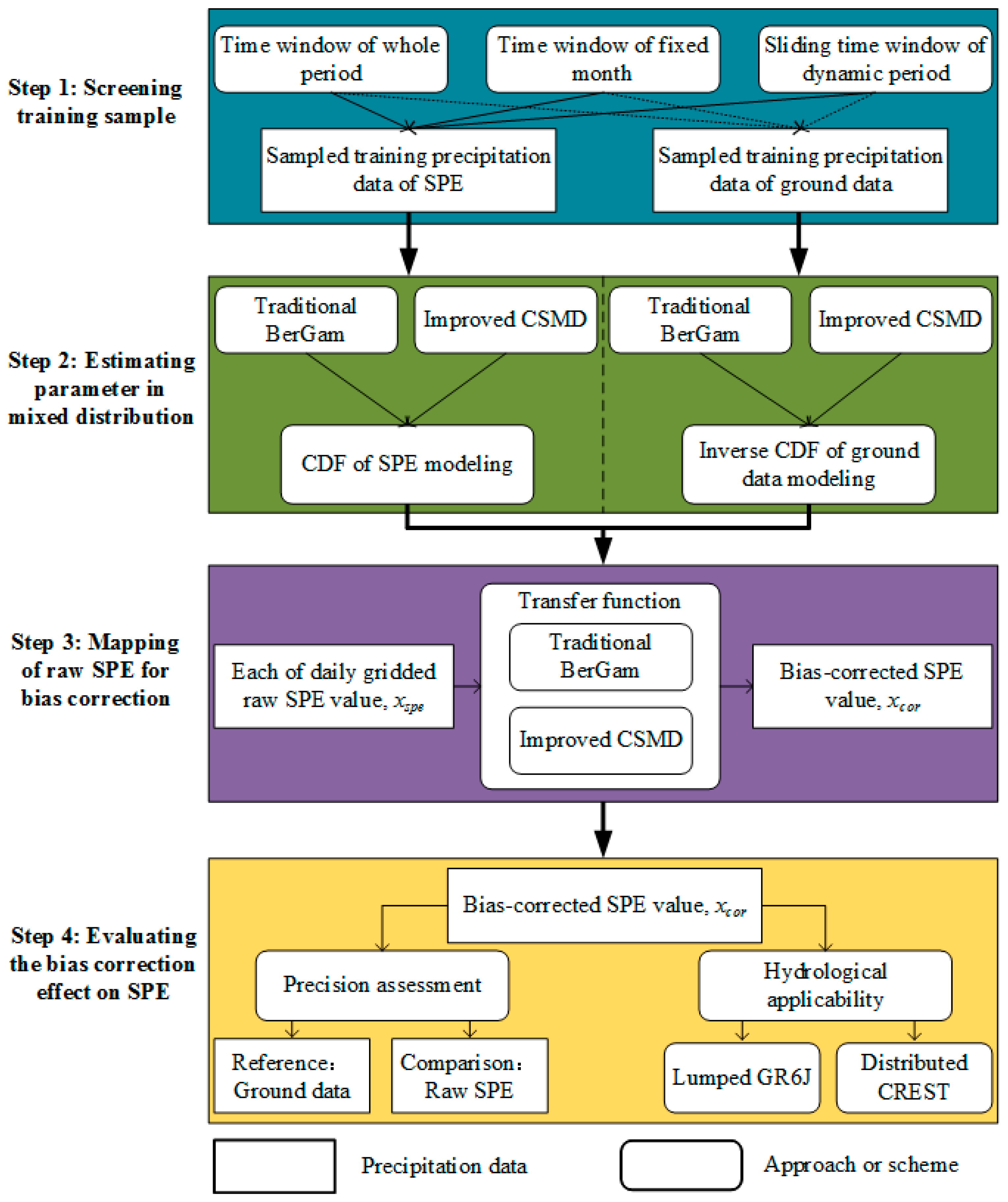
The method used in this study begins with the description of traditional BerGam and improved CSMD distribution mapping for bias correction of daily SPE, followed by three different time-window techniques used to pool precipitation samples for one CSMD implementation, then hydrological modeling of the GR6J and CREST models, and finally the evaluation indices for bias-corrected precipitation and resulting streamflow simulation. A four-step flowchart of the bias correction process, presented in Figure 3, was concentrated on estimating the parameters of mixed distribution in the second step and the mapping of SPE in the third step. The improvement of the developed method, which is incorporated in the deviating transfer function in Step 2 and 3 of Figure 3, focuses on the coupling of censored shifted statistical distribution and a mixture of gamma and generalized Pareto distributions to jointly model the probability of precipitation, precipitation intensity, and particularly the extremes. For the purpose of sampling precipitation data used to estimate the parameter set in BerGam or CSMD, the implementation of each bias correction is based on three time-windows, including the whole period window, monthly period window, and sliding window (see Step 1 in Figure 3).

3.1. Bias Correction of SPE Based on Distribution Mapping

It is assumed that the bias of SPE to be corrected in this study is constrained to the systematic bias resulting from, for instance, inaccurate measurement of the satellite sensor and noisy retrieval of the inversion algorithm. As the mainstream of bias correction, distribution mapping is frequently explored. The implementation of distribution mapping-based bias correction depends on the transfer function, a mapping or a statistical relationship from the biased SPE to observations. Whether the transfer function is skillful determines the efficiency of the bias correction. Therefore, the focus of the bias correction is to develop an available and powerful transfer function.
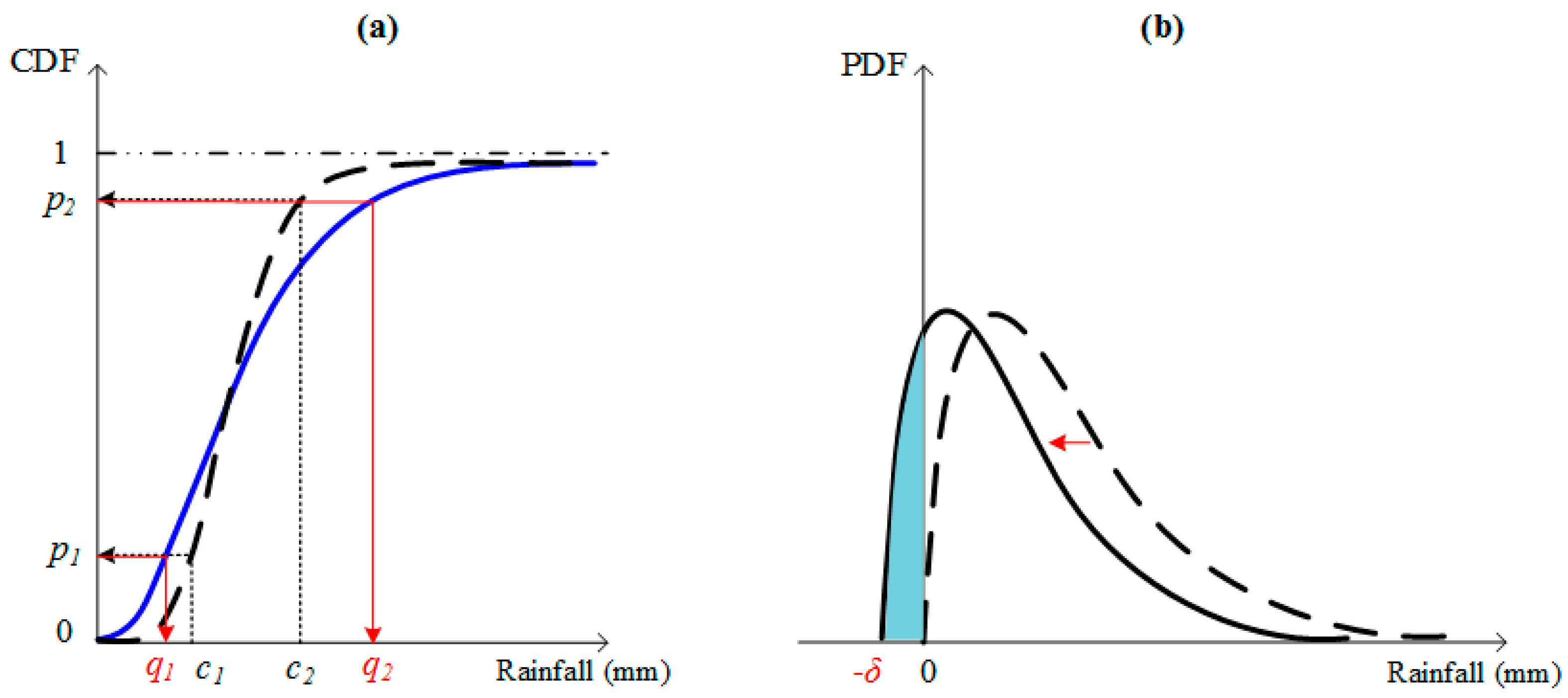
The statistical transformation in distribution mapping attempts to find a function that matches the IMERG-E precipitation variable Xspe, such that its new distribution approximates the distribution of the observed ground precipitation variable Xobs (see the schematic diagram of Figure 4a). The transfer function that controls how to obtain the corrected SPE can be formulated as:
x ˜ c o r = F o b s 1 ( F s p e ( x s p e ) )
where, x s p e is the raw IMERG-E data, x ˜ c o r is the corrected SPE processed by bias correction of distribution mapping, F s p e is the CDF of the raw IMERG-E, and F o b s 1 is the inverse CDF of the observation precipitation. In performing distribution mapping, each daily SPE value is ‘mapped’ into the corresponding quantile in the observation CDF.
Theoretically, both empirical and parametric CDF can be used to derive the transfer function. However, for empirical CDF, Equation (1) is only available for mapping values located in the historical range of the existing Xspe. Some extreme values out of the historical range cannot be derived under the context of empirical CDF. Therefore, to allow for extrapolation of the transfer function to unobserved precipitation intensities that might occur, a parametric distribution mapping approach instead of empirical CDF was chosen to solve the Equation (1) in this study.

3.1.1. Bernoulli-Gamma (BerGam) Distribution of Traditional Bias Correction

Traditionally, many studies modeling daily precipitation assume the parametric distribution F is a mixture including the Bernoulli (binomial) distribution to account for the mixed discrete/continuous nature of precipitation. While the Bernoulli distribution models the probability of precipitation occurrence giving a positive probability of precipitation being exactly zero, the gamma distribution is commonly used to depict precipitation intensity of being non-zero over a continuous value range [24,25]. In this way, a precipitation process can be separated into two steps using a total of three parameters. First, the probability of precipitation occurrence is modeled via a Bernoulli trial with the “success” parameter, p. Second, the continuous intensity of non-zero precipitation is modeled via a two-parameter gamma distribution with shape parameter k and scale parameter θ . The PDF of this BerGam mixture is defined as:
f ( x ) = { 1 p ,    x < t h r e s h o l d p × f g a m m a ( x ) ,   x > = t h r e s h o l d
where, the threshold (0.1 mm/d for this study) is used to classify zero and non-zero precipitation or dry and rainy days, and f g a m m a ( x ) denotes the PDF of the gamma distribution, given by:
f g a m m a ( x ) = { x k 1 1 θ k Γ ( k ) e x θ , x > 0 0 ,      o t h e r w i s e
The corresponding CDF is defined as:
F ( x ) = { 1 p ,    x < t h r e s h o l d p × F g a m m a ( x ) ,   x > = t h r e s h o l d
where, F g a m m a ( x ) is the CDF of the gamma distribution, given by:
F g a m m a ( x ) = { 1 Γ ( k ) γ ( k , x θ ) ,   x > 0 0 ,      o t h e r w i s e
In Equation (5), the mixture distribution of BerGam is determined by evaluating the three parameters p, k, and θ , and γ ( ) is the lower incomplete gamma function.

3.1.2. Censored Shifted Mixture Distribution of Improved Bias Correction

A more adequate and uniform mixed parametric distribution model, the censored shifted mixture distribution of gamma and generalized Pareto, i.e., CSMD, is proposed in this study. The improvement of CSMD is concentrated on two aspects of uniform format and the improved capture capability of extremely high values. Initially, CSMD allows simultaneously for model precipitation occurrence/nonoccurrence and intensity using a left-shifted continuous distribution instead of the multiple steps used in the BerGam mixture. Since the left-shifted gamma distribution permits negative values, the probability of precipitation can be represented by left-censoring the left-shifted gamma distribution at zero and replacing all negative values with zero. Specifically, an additional parameter δ is introduced to realize the censored and shifted distribution (Figure 4b). Following the work of Scheuerer and Hamill [26], the censored shifted CDF can be expressed as:
F ˜ ( x ) = { F ( x + δ ) ,   x 0 0 ,     x < 0
Denote by δ the distance of the shift of the distribution and let δ > 0 such that it ensures left shift.
The CSMD allocates F ( δ ) to the origin mass and can be generalized with PDF as:
f ˜ ( x ) = I { x = 0 } F ( δ ) + I { x > 0 } [ 1 F ( δ ) ] × f ( x + δ )
where I A denotes the indicator function of the set A.
Secondly, CSMD via introducing a typical extreme value distribution of generalized Pareto distribution avoids the deterioration of extreme values, as corrected using BerGam distribution mapping. Although the low and moderate precipitation intensities can be generally well-modeled, the extremely high values located in the tail of the gamma distribution are usually difficult to capture due to the highly light tails [31,50]. Therefore, the tail distribution associated with extreme values should be paid particular attention to. An extreme value distribution of generalized Pareto was applied to extreme values of high-precipitation intensity. Therefore, in the present study, the generalized Pareto is mixed with the previous gamma distribution to represent both the heavy and the low and moderate precipitation cases [33,51]. Subsequently, the censored shifted mixture of a gamma distribution for frequent precipitation intensities and a generalized Pareto distribution, particularly for the infrequent precipitation extremes, was developed. Thus, for f ˜ ( x ) in Equation (7), the shifted PDF expression of mixture distribution can be written as:
f ˜ ( x + δ ) = { ( 1 λ ) × f g a m m a ( x + δ ) + λ × f g p ( x + δ ) ,   x > 0 0 ,               o t h e r w i s e
where, λ is a weighting parameter assigned to f g p ( x ) , and f g p ( x ) is the PDF of the generalized Pareto distribution with shape parameter ξ and scale parameter σ . f g p ( x ) can be defined as:
f g p ( x ) = 1 σ [ 1 + ξ x σ ] ( 1 ξ 1 )
In summary, the CSMD approach developed above consists of a total of six parameters (two for gamma distribution, two for generalized Pareto distribution, one weighting coefficient, and one shift parameter) that need to be evaluated. The simulated annealing algorithm, capable of searching for the global optimal value, was applied to evaluate the parameter sets in CSMD for each of the three different time-window schemes (see detailed information in Albert et al. [52]).

3.2. Selection of the Time Window for Screening Precipitation Data

Three different time-windows, used to select the precipitation data pool in derivation of mixture distribution parameters of transfer functions BerGam and CSMD, were detected in this study, including the whole period window of the study time span, monthly period window, and sliding window. Considering the length of the data collected in the study and according to the recommendation of Smitha et al. [23], a 31-day sliding window technique was applied to pool precipitation data centered on each of the 365 days over the study period for the estimation of the parameter set in each of the BerGam and CSMD distributions. The sliding window technique facilitated the transfer function dynamic and downscaled the correcting factor from monthly to daily scale in correction of the raw IMERG-E. In contrast to the dynamic sliding window, the time windows screening in the whole or monthly periods are based on yearly and monthly correcting factors, respectively. Obviously, the sliding window is more flexible due to the evaluation of the time-varying parameters of BerGam and CSMD distribution mapping.

3.3. Streamflow Simulation Driven by Different Precipitation Inputs

To verify the hydrological effect of the bias-corrected SPE on the rainfall-runoff process, the lumped hydrological model GR6J (stands for mode‘le du Ge´nie Rural a‘ 6 parame‘tres Journalier) [53,54] and distributed Coupled Routing and Excess STorage (CREST) [55] were used in this study. GR6J is one of the conceptual rainfall-runoff models based on six free parameters (see Table 1). It was chosen because of the simple calibration and better performance than other model structures, including the previous versions of GR4J and GR5J models across various river-flow regimes [53].
In the model structure of GR5J, the water balance consists of a soil moisture accounting reservoir and a conceptual water exchange function (Fwe), denoted by:
F w e = X 2 × ( R X 3 X 5 )
where, X2 is the “groundwater” exchange coefficient, R and X3 represent the water level and the capacity of the routing store respectively, and X5 is a threshold parameter which accounts for the change in groundwater exchange within a year depending on R. Le Moine [56] introduced X5 into GR5J to improve the skill of the previous GR4J in interactions between surface and groundwater with regards to the low-flow simulation. Following this work, the sixth parameter X6, the coefficient for emptying exponential store, was added into GR5J to better consider these exchanges. The modified GR5J was called GR6J, which is used in this study. The performance of streamflow and peak-flood simulated via GR6J driven by different precipitation inputs, including the raw and corrected IMERG-E and ground reference precipitation, was analyzed.
As a grid-based distributed model, CREST calculates components of runoff generation using a variable infiltration capacity curve (VIC), which was proposed in Xinanjiang Model [57] and later incorprated in a VIC model [58]. The runoff generation components were represented by three connected linear reservoirs. Coupling runoff generation with routing components via feedback mechanisms facilitates a flexiable scalability in the space of the rainfall-runoff modeling, expecially in simulations at fine spatial resoluton, which is the typical characteristic of CREST [59]. SPE with high spatio-temporal resolution provides direct precipitation input for finely distributed modeling. The upgraded version 2.1 of CREST was introduced in this study to verify the hydrological effect of bias-corrected IMERG-E data in the distributed modeling case.

3.4. Evaluation Indices

In order to assess the performance of the proposed CSMD method in correcting SPE IMERG-E data, four statistical metrics were examined to quantify the difference between the corrected IMERG-E and the reference GDPA. These statistical metrics include mean absolute error (MAE), modified index of agreement (MD), modified Nash–Sutcliffe efficiency (mNSE) and Kling-Gupta efficiency (KGE). MAE is used to represent the mean residual bias between the corrected IMERG-E and the GDPA. MD and mNSE are indexes quantifying the scaled agreement of the corrected IMERG-E relative to the GDPA. KGE is a comprehensive measurement combining Pearson correlation and bias of both standard deviation and mean. Also, the performance of uncorrected raw IMERG-E with respect to these three metrics is presented for comparison. The mathematical expressions of the MAE, MD, mNSE, and KGE are listed in Table 2.
Further, in assessing the performance of the GR6J model in transforming precipitation into streamflow, the commonly used Nash–Sutcliffe efficiency (NSE) and relative deviation (RD) of the simulated to the observed streamflow were introduced. Please see Table 2 for the expression of these two metrics. It should be noted that the perfect matches of MAE and RD are 0, while the perfect matches of the other metrics are 1.

4. Results and Discussion

Initially in this section, the spatial and temporal variation of the raw satellite precipitation IMERG-E and IMERG-F over the Yangtze River basin was compared with ground analysis GDPA. Secondly, the performance of bias correction using CSMD and BerGam approaches exerting on the raw IMERG-E data was assessed using statistical metrics. Finally, the evaluation of the hydrological response of rainfall-runoff modeling to the corrected IMERG-E forcing was carried out via the GR6J and CREST models.

4.1. Assessment of the Raw IMERG-E and IMERG-F Against GDPA Data

The spatial distribution of the daily-averaged IMERG-E and IMERG-F against GDPA analysis over the Yangtze River basin during 1 April 2014–31 March 2018 is displayed in the Figure 5. The distribution pattern of IMERG-E and IMERG-F was broadly similar to that of GDPA, in which daily precipitation gradually increased along the northwest to the southeast direction. Whereas the IMERG-E and IMERG-F obviously underestimated the low precipitation values mainly in the west part of the Yangtze River basin, they overestimated the high values mainly in the east part. The areal-averaged daily mean and daily median precipitation of IMERG-E and IMERG-F during the four years from 1 April 2014–31 March 2018 were both relatively lower to GDPA (with daily mean values of 2.44 mm/d and 2.81 mm/d versus 2.95 mm/d for IMERG-E and IMERG-F against GDPA respectively, and daily median values of 0 mm/d and 0 mm/d versus 0.3 mm/d), while the daily standard deviation of IMERG-E and IMERG-F were both higher than that of GDPA (8.21 mm/d and 8.53 mm/d versus 7.21 mm/d), indicating a higher temporal variability.
To quantitatively assess the daily averaged discrepancies between the raw IMERG-E and IMERG-F against GDPA grid-by-grid, the differences between IMERG-E and resampled GDPA (Figure 5e) and between IMERG-F and resampled GDPA (Figure 5f) are presented. It can be clearly observed from Figure 5e,f that the difference of IMERG-E showed a larger range (−3.18–2.27 mm) over the basin, especially a larger negative difference in the mid-west region, compared to IMERG-F (with range of −2.33–2.1 mm). The median and standard deviation of the daily averaged difference in IMERG-E and GDPA among all grids in the basin were −0.19 mm and 0.63 mm respectively, contrasted to those for IMERG-F with values of 0.25 mm and 0.52 mm. Smaller range and standard deviation associated with fluctuation of the difference in IMERG-F indicated higher precision of IMERG-F, due to merging with monthly GPCC gauge data, than that of IMERG-E. Previous studies on SPE evaluation over the Yangtze River basin demonstrated that IMERG-E performed better than (or comparably with) the other widely used SPE. The differences between GPM IMERG-F and GPM IMERG-E against ground data in this study were comparable with those between TMPA 3B42V7 and TMPA 3B42RT against ground data and significantly lower than those between CMORPH product and ground data in Li et al. [60] and Shen et al. [46]. Li et al. [61] reported that IMERG-F showed a higher Correction Coefficient and Root Mean Square Error against ground data over the Yangtze River basin, when compared with CMORPH and PERSIANN-CDR products.

4.2. Performance of Corrected IMERG-E using CSMD and BerGam

4.2.1. Parameter Estimation of Two Bias Correction Approaches

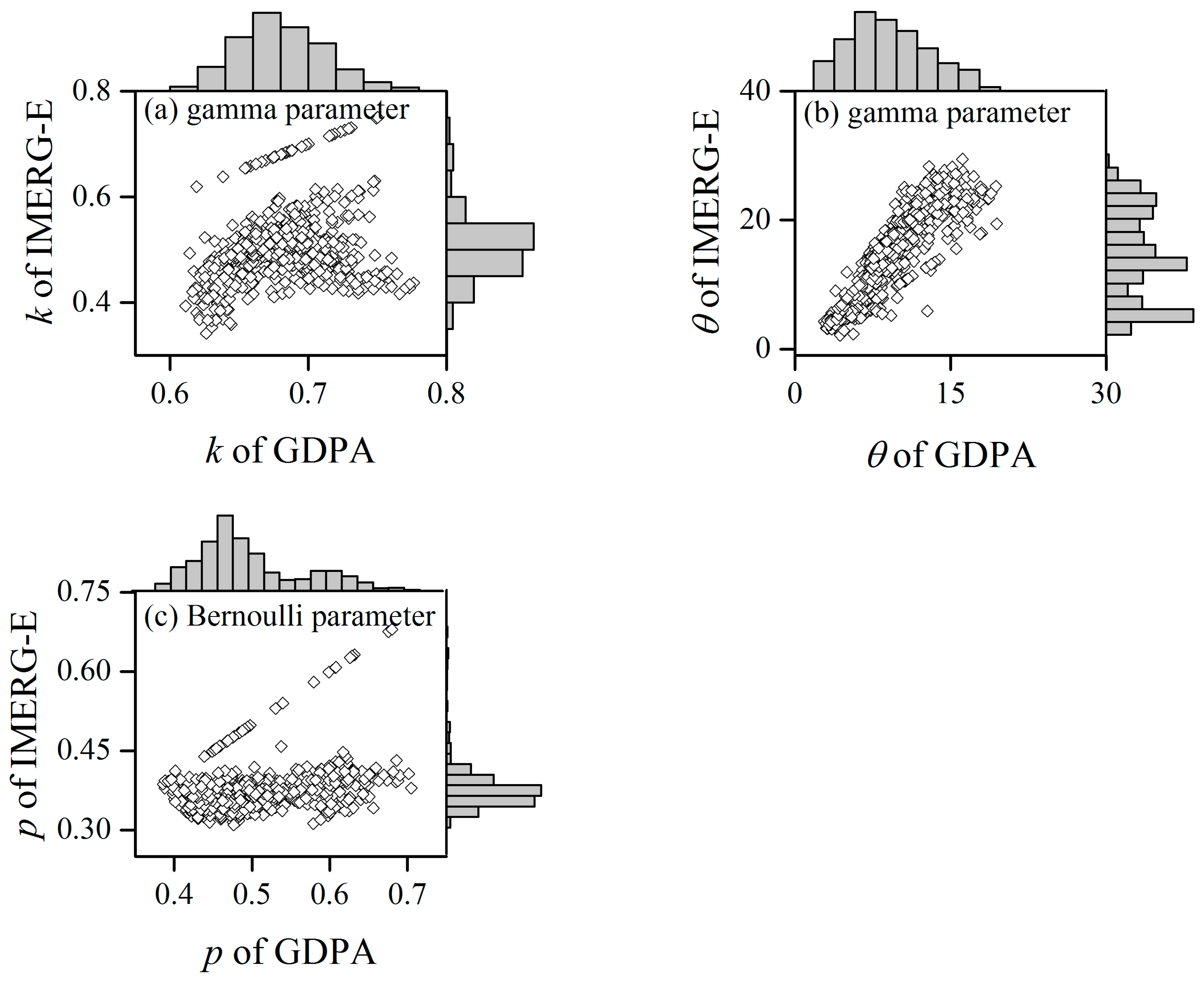
For SPE to be corrected, given the definition of the transfer function of distribution mapping, the important procedure is to estimate the parameter sets in the transfer function of traditional BerGam and improved CSMD (see Step 2 of Figure 3). Figure 6 displays the scatters and histograms of each optimal parameter of BerGam estimated for IMERG-E and corresponding GDPA data at all grids in the basin. Figure 6 depicts the estimation range and degree of aggregation for each parameter over all grids. For example, IMERG-E showed smaller shape parameter k and higher scale parameter θ in gamma distribution, and smaller p parameter in Bernoulli distribution at most grids.
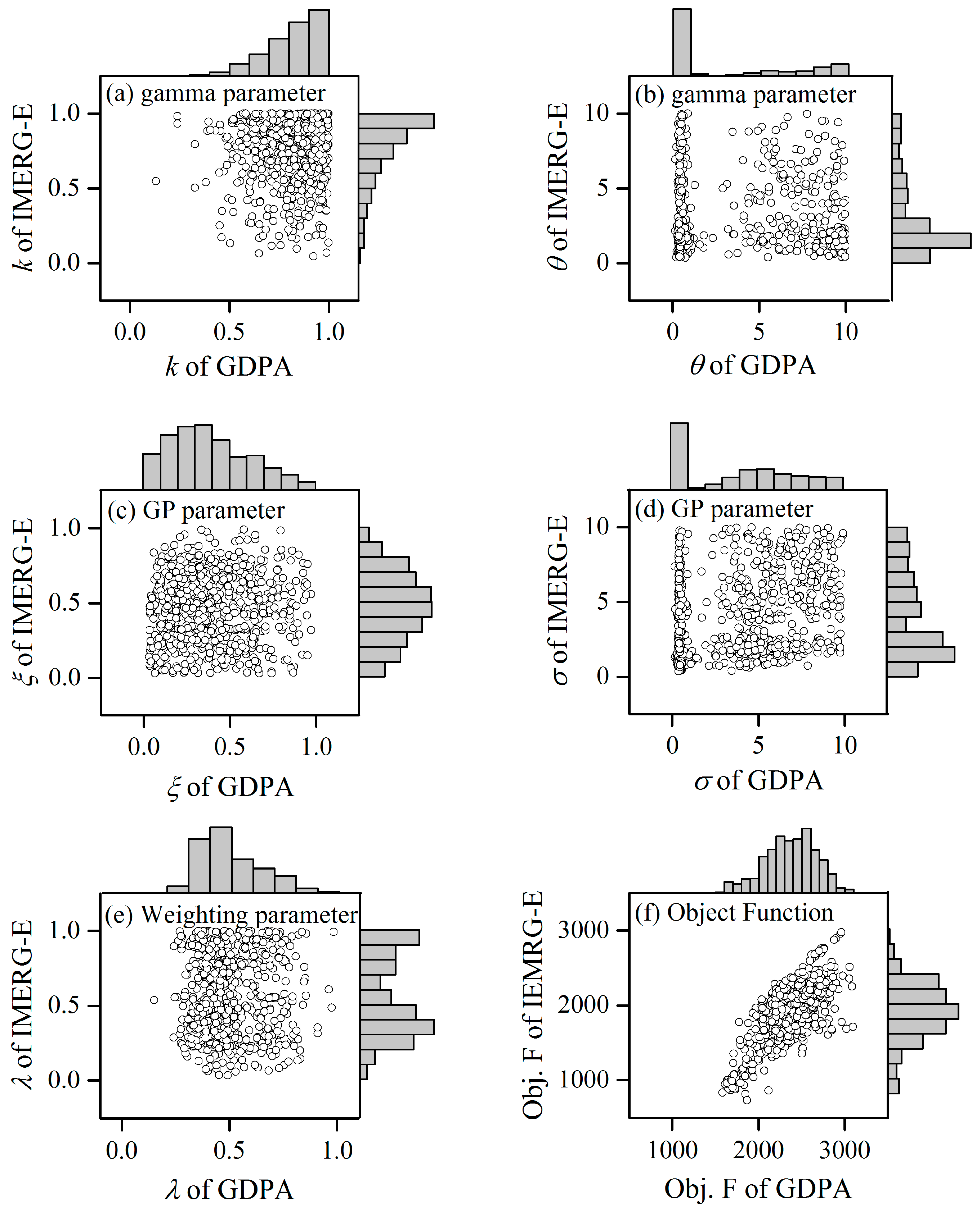
Similar with Figure 6 of the BerGam case, Figure 7 displays the estimated parameters in the improved CSMD distribution mapping approach over all grids. The degrees of aggregation of parameters in CSMD (Figure 7a–e) were relatively lower than those in BerGam. Furthermore, the values of objective function (used as a criteria of optimization in the simulated annealing algorithm) are presented in Figure 7f, which verified the effectiveness of the parameter optimization used in this study.

4.2.2. Comparison of CSMD Correction with BerGam Correction

To statistically quantify the bias correction effect on IMERG-E from multiple aspects, the performance of bias-corrected IMERG-E using CSMD and BerGam methods was represented by the metrics of MAE, MD, mNSE, and KGE mentioned above. These four indexes present an integrated understanding of the difference in IMERG against GDPA from relative/absolute residual errors to comprehensive evaluation. Figure 8 presents the boxplots of these metrics calculated in each grid. It could be clearly observed that either improved CSMD correction or traditional BerGam correction reduced the discrepancy of raw satellite precipitation and ground analysis and significantly enhanced the precision of the precipitation series at most grids. In addition, the corrected IMERG-E via CSMD mapping approach as a transfer function generally performed better than that via traditional BerGam mapping. Specifically, the mean and quartile MAE values of IMERG-E corrected by CSMD were much lower compared to the corresponding values of BerGam. For example, the means of MAE for CSMD- and BerGam-corrected IMERG were 2.35–2.52 mm and 2.75–2.79 mm among three time-window schemes respectively, while the median values of MAE for CSMD- and BerGam-corrected IMERG-E were around 2.45 mm and 2.81 mm, respectively. Similarly, the CSMD-corrected IMERG-E was superior to the BerGam-corrected IMERG-E in terms of MD and mNSE metrics. As for IMERG-E, the KGE exhibited unsatisfying results with values lower than 0.1, even negative, mainly over the northwest part of the basin. For KGE, an index of comprehensive assessment, the CSMD correction performs comparatively well overall with BerGam, with the exceptional case of taking the whole period as a time window. The CSMD-corrected IMERG-E outperformed BerGam-corrected IMERG-E in metrics of MAE, MD, and mNSE, while performing comparatively with BerGam-corrected IMERG-E in terms of the KGE metric. This is associated with the different emphases of the four metrics, that MAE, MD, and mNSE aim at the quantification of deviation between each pair of two input precipitation series and KGE aims at a relationship of the whole trend between the two series. These results suggested that the improvement of the CSMD correction to IMERG-E was mainly concentrated on the reduction of deviation of the biased raw IMERG-E to the reference data. As a comparator of IMERG-E, the post-real-time IMERG-F data performed better than the raw IMERG-E towards MD and KGE metrics, while performing worse than IMERG-E towards MAE and mNSE metrics. On the other hand, both the BerGam-corrected and CSMD-corrected IMERG-E performed much better than IMERG-F towards all four metrics, shown in Figure 8. These results indicated that not only the precision of corrected IMERG-E using BerGam and CSMD was higher than the raw IMERG-E, but also the effect that bias correction exerted on the IMERG-E surpassed the post-processing of IMERG-F by merging monthly GPCC gauge data.
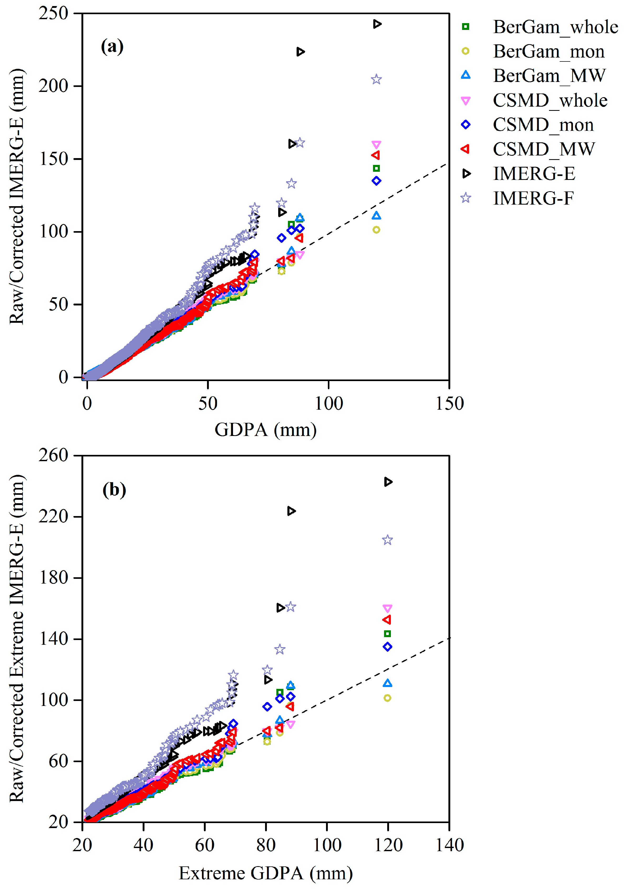
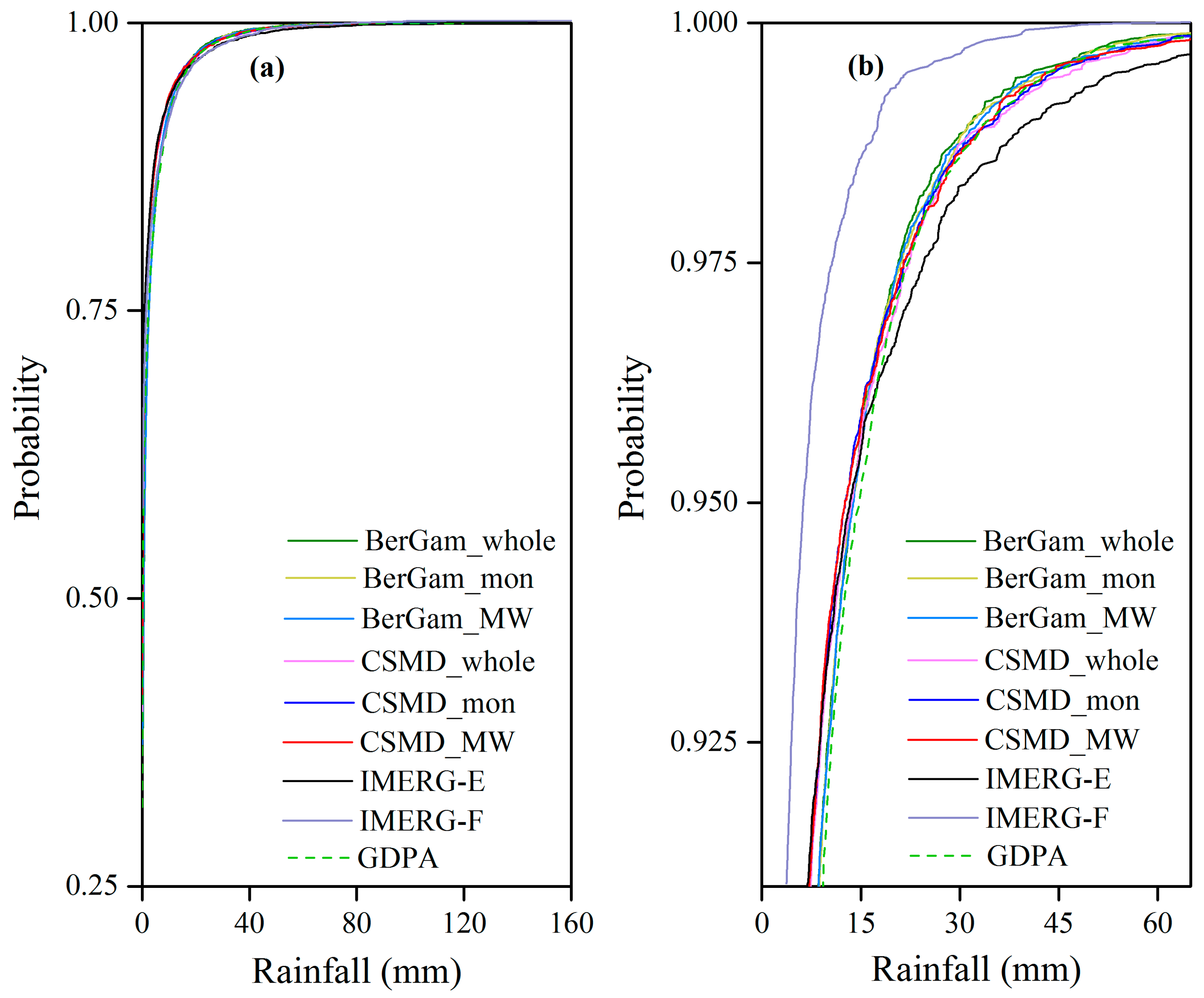
The Q-Q plot of raw and corrected daily IMERG-E and IMERG-F against GDPA during the four years of the study period at 100 randomly selected grids is shown in Figure 9a, which is a graphical way to diagnostic agreement between satellite precipitation and ground reference. Compared to the large divergence of the raw IMERG-E and the post-corrected IMERG-F to the 1:1 line (where the perfect fit with GDPA is), the corrected IMERG-E including using both the CSMD and BerGam correction kept relatively consistent with the 1:1 line. Besides, the CSMD-corrected IMERG-E was located more closely around the 1:1 line. This also verifies the contribution of the correction, especially the CSMD correction, to the reduction of bias in the raw satellite precipitation data. Furthermore, to investigate the bias correction contribution to the raw IMERG-E from the frequency of the daily precipitation distribution, the CDF of each bias-corrected daily IMERG-E during the study period was computed at 100 randomly selected grids over the basin (Figure 10). Figure 10b enlarged the top of the CDF curves ranging from 0.91 to 1 where the difference among eight categories of precipitation was considerable. Figure 10 shows that the bias correction adjusted the substantial underestimation of low and median precipitation and the overestimation of high precipitation.
The difference caused by different time-window schemes was very insignificant, although a slight improvement existed in some quantiles of IMERG-E precipitation after the CSMD and BerGam correction. The median and 75 and 99 percentiles of MAE and MD for BerGam correction were almost the same among the three time-window schemes, while these three quantiles in mNSE and KGE metrics obtained a slight increase because of the introduction of the sliding window technique. As for the case of CSMD correction, although the corrected IMERG-E obtained some improvement in the monthly period and sliding window schemes, compared with the whole time period window scheme, the performance in the sliding window scheme was very comparative to that using the monthly time-window scheme. In summary, there was a slight improvement obtained by using the dynamic sliding window scheme. This is inconsistent with the previous result that showed that obvious improvement in the performance of corrected precipitation by introducing the sliding window scheme was detected relative to the monthly period window [23]. This contrast may be associated with the length limitation of the precipitation data used in this study since the robust sliding window technique needs the support of substantial data.

4.2.3. Performance of Corrected Extreme IMERG-E against GDPA

The extremely high precipitation is one of the focuses in precipitation bias correction using distribution mapping due to the extremely low probability of high values located in the tail of the distribution (see Figure 4b). Therefore, the effect of bias correction on extreme precipitation attracted particular attention. The Q-Q plot of extremely high precipitation (greater than 97.5% quantile with threshold values ranging from 20.68–24.55 mm) for raw and corrected IMERG-E against the corresponding extreme GDPA data was displayed in Figure 9b. For the extreme part of corrected precipitation, the CSMD correction using the sliding window scheme generally obtained best-fitness with the GDPA data, followed by the CSMD correction using the whole time period window scheme. In addition to the Q-Q plot, the empirical CDF of precipitation in Figure 10b, focusing on the change of CDF ranging 0.91–1, can also be used to analyze the goodness-of-fit for extreme precipitation correction. From the Figure 10b, it can be observed that the corrected IMERG-E curves, especially for the result associated with CSMD correction, keep well-consistent with the GDPA curve in the precipitation range of greater than about 20 mm/d, although the curves of BerGam-corrected IMERG-E series performed better than those of the CSMD correction in the range of 13–20 mm/d. In summary, the result in Figure 10b demonstrated that the CSMD correction is more skillful in correction the extremely high precipitation intensities.
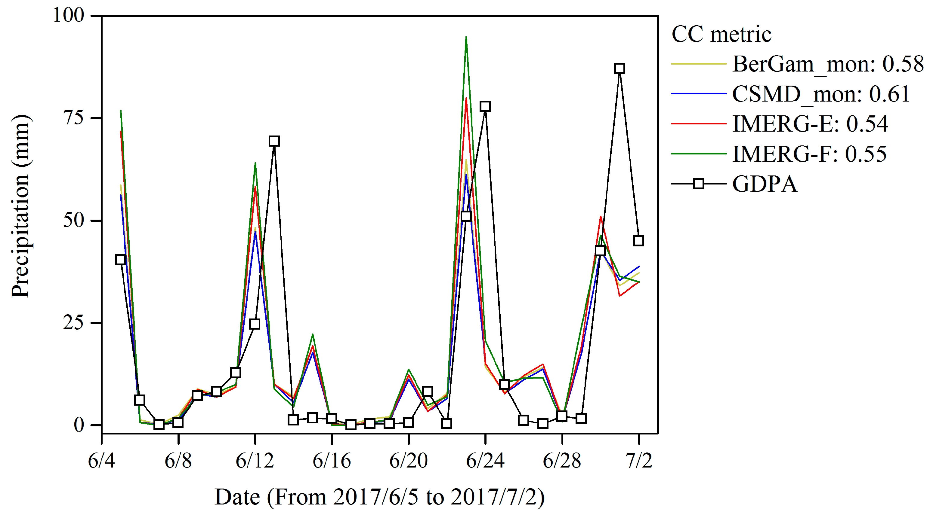
A typical storm event occurring at a grid (116.5°E, 29.5°N) of eastern area during 5 June 2017–2 July 2017 was taken as an example to verify the bias correction effect on summer heavy rainfall. Figure 11 exhibits the temporal process of bias-corrected IMERG-E, post-processed IMERG-F, and GDPA. The CC metric of CSMD-corrected precipitation with GDPA in this storm event was the highest (0.61), followed by BerGam (0.58). Although the CC value of IMERG-F (0.55) was slightly higher than that of the raw IMERG-E (0.54), it was significantly lower than those of the precipitation corrected using both BerGam (0.58) and CSMD (0.61). These results also suggested that bias-corrected extreme precipitation outperformed the post-processed extreme precipitation in IMERG-F. The time lag between SPE (i.e., IMERG-E and IMERG-F) from NASA and GDPA from NMIC-CMA may result from different timing. However, the relative relations of corrected IMERG-E with the raw IMERG-E or with IMERG-F remain unchanged, although the time lag may lead to a systematic reduction of evaluation performance when assessing the precision for each of SPE against GDPA.

4.3. Evaluation of Simulated Streamflow Driven by Corrected IMERG-E

Theoretically, the improvement of SPE that resulted from bias correction can enhance the hydrological simulation and forecast via rainfall-runoff process. Thus, the bias-corrected IMERG-E using both CSMD and BerGam as transfer functions for distribution mapping was further used as hydrological model input to quantify their contributions and error propagations to the streamflow simulation.
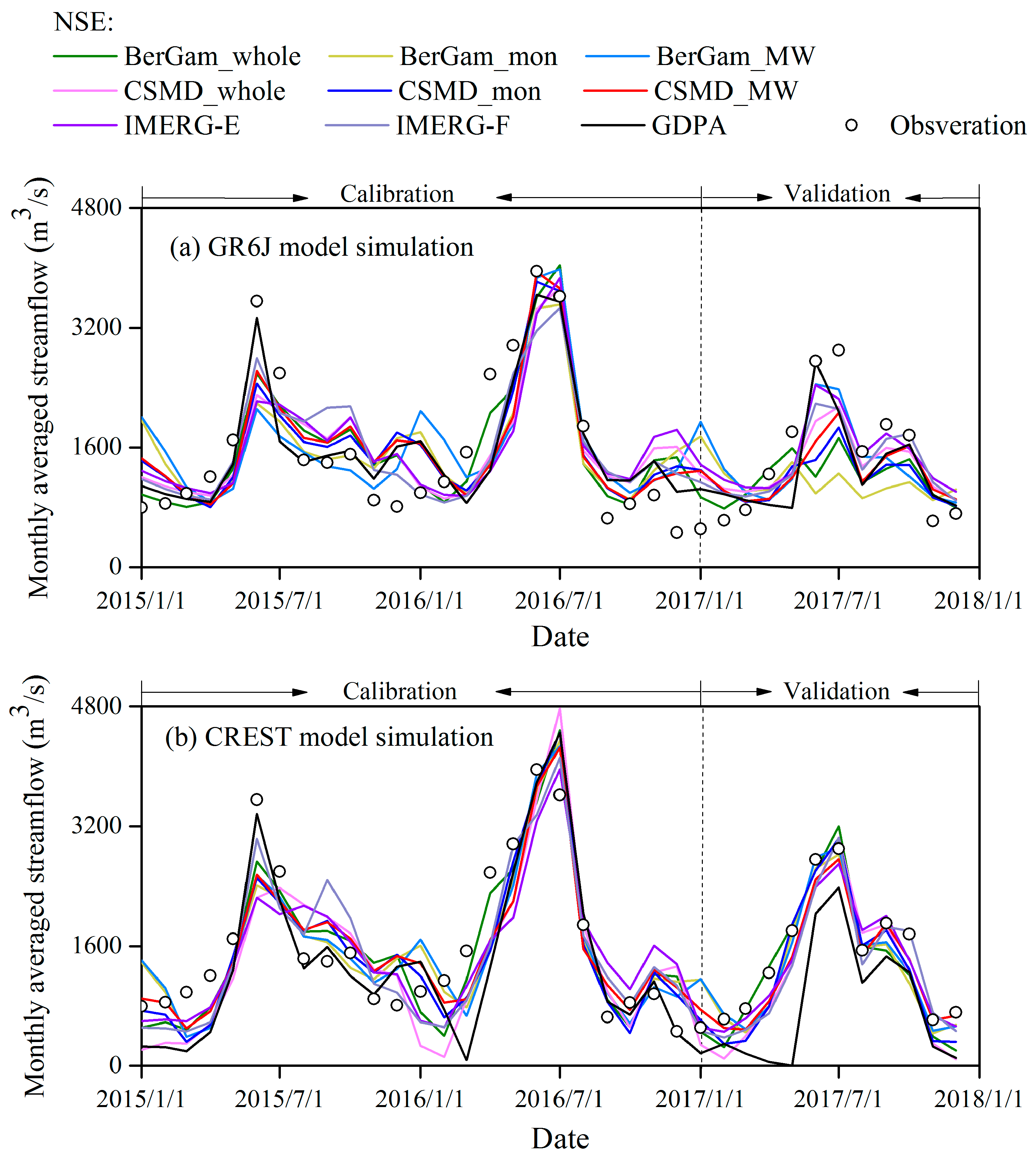
The streamflow simulation of Wulong station at the outlet of Wujiang River basin individually via the lumped GR6J and distributed CREST forced by nine precipitation inputs including one raw and six bias-corrected IMERG-E precipitation, post-real-time IMERG-F, and one ground reference GDPA during 1 April 2014–31 December 2017 was evaluated. Figure 12 presents the monthly-accumulated hydrographs of the simulated streamflow. The summary of NSE, r, and RD metrics between simulated streamflow and observed streamflow in calibration and validation periods was listed in Table 3. NSE and RD were used to quantify the deviation of SPE from GDPA, while r was used to depict the global correlation between SPE and GPDA. Although there existed no completely uniform pattern of streamflow simulation precision in BerGam and CSMD, the streamflow simulation driven by CSMD-corrected IMERG-E outperformed that driven by BerGam-corrected IMERG-E in more cases of calibration and validation. Specifically, taking NSE for example, the simulated streamflow of GR6J driven by BerGam deteriorated in validation period (NSE ranging in −0.15–0.40) even obtained useless results with negative NSE in the case of BerGam_mon, although it performed well in the calibration period (NSE ranging from 0.47–0.62). The performance of rainfall-runoff modeling via GR6J in both the calibration and validation periods was acceptable with NSE ranging from 0.51–0.56 and from 0.35–0.51, respectively. Similarly, with GR6J, the performance of CSMD-driven streamflow simulation via CREST in the validation period, as indicated by the NSE index, was overall better than that of the BerGam-driven results (0.62–0.74 versus 0.66–0.68 for the CSMD and BerGam correction respectively), indicating the higher prediction capability of CSMD relative to BerGam. The modeling precision associated with IMERG-F was overall slightly lower than that with CSMD-MW, which performed best among all nine precipitation inputs. Furthermore, the simulation of CREST obtained better performance than that of GR6J, and the unreliable modeling with negative NSE values occurred in GR6J, demonstrating that the distributed CREST model was more robust than the lumped GR6J in this study. If it is assumed that higher performance (shadowed numbers in Table 3) of two or three metrics among NSE, r, and RD appeared in the same model running, then the conclusion is the same with the evaluation using NSE only, although the order of r or RD was not completely the same as ranked NSE in the shadow grids of Table 3. In general, the hydrological effect that the CSMD correction exerted on IMERG-E driving GR6J and CREST rainfall-runoff modeling outperformed that of the BerGam correction.
In addition, the performance of hydrological modeling with respect to NSE in the Wujiang River basin is relatively low, especially for using the simulation of GR6J (NSE 0.62). The reason for low performance may be the impact of intensive human activities, including reservoirs and dams [62], hydroelectric power stations [63], and metal mines built in this area [64], and the specific environment of Karst geomorphology and hydrogeology [63] in this part of the Wujiang River basin. Although these anthropic activities and natural features potentially impact the trend of the initial streamflow and may result in the unsatisfying hydrological modeling, this is beyond the scope of this study. Nevertheless, the streamflow can also be used to roughly verify the bias-correction effect of satellite precipitation on hydrology modeling. Moreover, the SPE data used in this study were from less than four years (45 months), restricted by the availability of IMERG SPE. Therefore, the short period of hydrological modeling corresponding to IMERG SPE may potentially exert a negative effect on the performance of the streamflow simulation in the Wulong outlet of the Wujiang River basin. Thus, further verification with longer data available for IMERG SPE in the near future is expected.

5. Summary and Conclusions

In the present study, with respect to the bias correction of daily satellite precipitation estimates, an improved distribution mapping method coupling a censored shifted distribution with a mixture of gamma and generalized Pareto distributions (CSMD) was established. The comparison of bias correction using CSMD as a transfer function and the traditional Bernoulli-gamma mixture distribution (BerGam) as a transfer function was carried out by application to correct the satellite precipitation estimates of IMERG-E over the Yangtze River basin. The performance of bias-corrected IMERG-E and IMERG-E against ground gridded analysis (GDPA) was represented using the evaluation metrics of MAE, MD, mNSE, and KGE. Moreover, the effect of hydrological application with bias correction was quantified. The primary conclusions were derived as follows:
(1)
Both correction approaches of the improved CSMD and the traditional BerGam can significantly reduce the systematic bias of the satellite precipitation product IMERG-E. Furthermore, CSMD was superior to BerGam with respect to the deviation-dependent metrics of MAE, MD, and mNSE for precipitation assessment.
(2)
CSMD performed better in correction of the extremely high precipitation, which is the difficulty of the distribution mapping commonly used, as compared to the BerGam correction. This improvement in extreme values is mainly due to the mixture consisting of the generalized Pareto distribution focusing on the extreme value modeling.
(3)
The IMERG-E bias correction for CSMD via the sliding window scheme obtained slight improvement, compared to the whole period and monthly period time-window schemes, while there was no significant change among the three time-window schemes for BerGam.
(4)
The streamflow simulation driven by the CSMD-corrected IMERG-E outperformed that driven by the BerGam-corrected IMERG-E in more cases of calibration and validation (NSE of GR6J in validation: 0.44–0.51 versus −0.15–0.4 for CSMD and BerGam, respectively. NSE of CREST in validation: 0.62–0.74 versus 0.66–0.68). The distributed CREST model was more robust than the lumped GR6J in verifying the bias correction effect on satellite precipitation IMERG-E for modeling and prediction.
Overall, the established CSMD bias correction method, featured with both jointly modeling precipitation occurrence and intensity and with particular attention paid to the extreme modeling, is expected to be more capable in correction of the daily satellite precipitation estimates relative to the traditional BerGam. Further modifications of the CSMD method can consider more mixture components of parametrical distributions and enhance the computation efficiency in parameter optimization, while a larger dataset is needed to test the efficacy and robustness of the proposed method.
As SPE find a broad range of applications in hydrological modeling, the advanced statistical bias correction brings a promising reduction of the systematic bias of SPE, leading to a more reliable hydrological forecast. Thus, the CSMD method proposed in this study is recommended to test and apply to other SPE products and other regions lacking ground precipitation measurements.

Author Contributions

Q.M. and L.X. designed the experiments; Q.M. conducted the experiments and wrote the original draft; J.X. and C.-Y.X. provided helpful suggestions; B.X. and H.Y. polished the manuscript.

Funding

This research was financially supported jointly by the National Key Research and Development Program of China (Grants No. 2017YFC0405901), National Natural Science Foundation of China (Grants Nos. 41890822 and 51525902), the Research Council of Norway (FRINATEK Project 274310), and the Ministry of Education “111 Project” Fund of China (B18037).

Acknowledgments

The authors would like to thank the editor, associate editor, and anonymous reviewers for processing our manuscript. The authors’ gratitude is also extended to the Goddard Space Flight Center’s PMM Science Team of NASA, China Meteorological Data Service Center, and Hydrologic Bureau of the Ministry of Water Resources of China for providing IMERG, ground precipitation, and streamflow data, respectively.

Conflicts of Interest

The authors declare no conflict of interest.

References

  1. Tapiador, F.J.; Turk, F.J.; Petersen, W.; Hou, A.Y.; García-Ortega, E.; Machado, L.A.; Angelis, C.F.; Salio, P.; Kidd, C.; Huffman, G.J. Global precipitation measurement: Methods, datasets and applications. Atmos. Res. 2012, 104, 70–97. [Google Scholar] [CrossRef]
  2. Collins, M.; AchutaRao, K.; Ashok, K.; Bhandari, S.; Mitra, A.K.; Prakash, S.; Srivastava, R.; Turner, A. Observational challenges in evaluating climate models. Nat. Clim. Chang. 2013, 3, 940–941. [Google Scholar] [CrossRef]
  3. Ashouri, H.; Hsu, K.; Sorooshian, S.; Braithwaite, D.K.; Knapp, K.R.; Cecil, L.D.; Nelson, B.R.; Prat, O.P. PERSIANN-CDR: Daily precipitation climate data record from multisatellite observations for hydrological and climate studies. Bull. Am. Meteorol. Soc. 2015, 96, 69–83. [Google Scholar] [CrossRef]
  4. Hou, A.Y.; Kakar, R.K.; Neeck, S.; Azarbarzin, A.A.; Kummerow, C.D.; Kojima, M.; Oki, R.; Nakamura, K.; Iguchi, T. The global precipitation measurement mission. Bull. Am. Meteorol. Soc. 2014, 95, 701–722. [Google Scholar] [CrossRef]
  5. Ma, Y.; Hong, Y.; Chen, Y.; Yang, Y.; Tang, G.; Yao, Y.; Long, D.; Li, C.; Han, Z.; Liu, R. Performance of optimally merged multisatellite precipitation products using the dynamic Bayesian model averaging scheme over the Tibetan Plateau. J. Geophys. Res. Atmos. 2018, 123, 814–834. [Google Scholar] [CrossRef]
  6. Vernimmen, R.; Hooijer, A.; Aldrian, E.; Van Dijk, A. Evaluation and bias correction of satellite rainfall data for drought monitoring in Indonesia. Hydrol. Earth Syst. Sci. 2012, 16, 133–146. [Google Scholar] [CrossRef] [Green Version]
  7. Ma, Y.; Tang, G.; Long, D.; Yong, B.; Zhong, L.; Wan, W.; Hong, Y. Similarity and error intercomparison of the GPM and its predecessor-TRMM Multisatellite Precipitation Analysis using the best available hourly gauge network over the Tibetan Plateau. Remote Sens. 2016, 8, 569. [Google Scholar] [CrossRef]
  8. Wright, D.B.; Kirschbaum, D.B.; Yatheendradas, S. Satellite Precipitation Characterization, Error Modeling, and Error Correction Using Censored Shifted Gamma Distributions. J. Hydrometeorol. 2017, 18, 2801–2815. [Google Scholar] [CrossRef]
  9. Worqlul, A.W.; Ayana, E.K.; Maathuis, B.H.; MacAlister, C.; Philpot, W.D.; Leyton, J.M.O.; Steenhuis, T.S. Performance of bias corrected MPEG rainfall estimate for rainfall-runoff simulation in the upper Blue Nile Basin, Ethiopia. J. Hydrol. 2018, 556, 1182–1191. [Google Scholar] [CrossRef]
  10. Tang, G.; Ma, Y.; Long, D.; Zhong, L.; Hong, Y. Evaluation of GPM Day-1 IMERG and TMPA Version-7 legacy products over Mainland China at multiple spatiotemporal scales. J. Hydrol. 2016, 533, 152–167. [Google Scholar] [CrossRef]
  11. Xu, R.; Tian, F.; Yang, L.; Hu, H.; Lu, H.; Hou, A. Ground validation of GPM IMERG and TRMM 3B42V7 rainfall products over southern Tibetan Plateau based on a high-density rain gauge network. J. Geophys. Res. Atmos. 2017, 122, 910–924. [Google Scholar] [CrossRef]
  12. Huffman, G.J.; Bolvin, D.T.; Nelkin, E.J. Integrated Multi-satellitE Retrievals for GPM (IMERG) technical documentation. NASA/GSFC Code 2015, 612, 47. [Google Scholar]
  13. Ma, Q.; Xiong, L.; Liu, D.; Xu, C.; Guo, S. Evaluating the Temporal Dynamics of Uncertainty Contribution from Satellite Precipitation Input in Rainfall-Runoff Modeling Using the Variance Decomposition Method. Remote Sens. 2018, 10, 1876. [Google Scholar] [CrossRef]
  14. Huffman, G.J.; Bolvin, D.T.; Braithwaite, D.; Hsu, K.; Joyce, R.; Xie, P.; Yoo, S.H. Algorithm Theoretical Basis Document (ATBD) Version 5.1. Available online: https://pmm.nasa.gov/sites/default/files/document_files/IMERG_ATBD_V5.1b.pdf (accessed on 5 January 2019).
  15. Guo, H.; Chen, S.; Bao, A.; Behrangi, A.; Hong, Y.; Ndayisaba, F.; Hu, J.; Stepanian, P.M. Early assessment of integrated multi-satellite retrievals for global precipitation measurement over China. Atmos. Res. 2016, 176, 121–133. [Google Scholar] [CrossRef]
  16. Gervais, M.; Tremblay, L.B.; Gyakum, J.R.; Atallah, E. Representing extremes in a daily gridded precipitation analysis over the United States: Impacts of station density, resolution, and gridding methods. J. Clim. 2014, 27, 5201–5218. [Google Scholar] [CrossRef]
  17. Abera, W.; Brocca, L.; Rigon, R. Comparative evaluation of different satellite rainfall estimation products and bias correction in the Upper Blue Nile (UBN) basin. Atmos. Res. 2016, 178, 471–483. [Google Scholar] [CrossRef]
  18. Teng, J.; Potter, N.J.; Chiew, F.; Zhang, L.; Wang, B.; Vaze, J.; Evans, J.P. How does bias correction of regional climate model precipitation affect modelled runoff? Hydrol. Earth Syst. Sci. 2015, 19, 711–728. [Google Scholar] [CrossRef] [Green Version]
  19. Li, W.; Duan, Q.; Miao, C.; Ye, A.; Gong, W.; Di, Z. A review on statistical postprocessing methods for hydrometeorological ensemble forecasting. Wiley Interdiscip. Rev. Water 2017, 4, e1246. [Google Scholar] [CrossRef]
  20. Müller, M.F.; Thompson, S.E. Bias adjustment of satellite rainfall data through stochastic modeling: Methods development and application to Nepal. Adv. Water Resour. 2013, 60, 121–134. [Google Scholar] [CrossRef] [Green Version]
  21. Gumindoga, W.; Rientjes, T.; Haile, A.T.; Makurira, H.; Reggiani, P. Bias correction schemes for CMORPH satellite rainfall estimates in the Zambezi River Basin. Hydrol. Earth Syst. Sci. Discuss. 2016, 1–36. [Google Scholar] [CrossRef]
  22. Yang, Z.; Hsu, K.; Sorooshian, S.; Xu, X.; Braithwaite, D.; Verbist, K.M. Bias adjustment of satellite-based precipitation estimation using gauge observations: A case study in Chile. J. Geophys. Res. Atmos. 2016, 121, 3790–3806. [Google Scholar] [CrossRef]
  23. Smitha, P.S.; Narasimhan, B.; Sudheer, K.P.; Annamalai, H. An improved bias correction method of daily rainfall data using a sliding window technique for climate change impact assessment. J. Hydrol. 2018, 556, 100–118. [Google Scholar] [CrossRef]
  24. Dunn, P.K. Occurrence and quantity of precipitation can be modelled simultaneously. Int. J. Climatol. 2004, 24, 1231–1239. [Google Scholar] [CrossRef] [Green Version]
  25. Cannon, A.J. Probabilistic multisite precipitation downscaling by an expanded Bernoulli–Gamma density network. J. Hydrometeorol. 2008, 9, 1284–1300. [Google Scholar] [CrossRef]
  26. Scheuerer, M.; Hamill, T.M. Statistical postprocessing of ensemble precipitation forecasts by fitting censored, shifted gamma distributions. Mon. Weather Rev. 2015, 143, 4578–4596. [Google Scholar] [CrossRef]
  27. Baran, S.; Nemoda, D. Censored and shifted gamma distribution based EMOS model for probabilistic quantitative precipitation forecasting. Environmetrics 2016, 27, 280–292. [Google Scholar] [CrossRef] [Green Version]
  28. Zhang, Y.; Wu, L.; Scheuerer, M.; Schaake, J.; Kongoli, C. Comparison of Probabilistic Quantitative Precipitation Forecasts from Two Postprocessing Mechanisms. J. Hydrometeorol. 2017, 18, 2873–2891. [Google Scholar] [CrossRef]
  29. Schleiss, M.; Chamoun, S.; Berne, A. Nonstationarity in intermittent rainfall: The “dry drift”. J. Hydrometeorol. 2014, 15, 1189–1204. [Google Scholar] [CrossRef]
  30. Baxevani, A.; Lennartsson, J. A spatiotemporal precipitation generator based on a censored latent Gaussian field. Water Resour. Res. 2015, 51, 4338–4358. [Google Scholar] [CrossRef] [Green Version]
  31. Volosciuk, C.D.; Maraun, D.; Vrac, M.; Widmann, M. A combined statistical bias correction and stochastic downscaling method for precipitation. Hydrol. Earth Syst. Sci. 2017, 21, 1693–1719. [Google Scholar] [CrossRef] [Green Version]
  32. Wu, X.; Wang, Z.; Guo, S.; Liao, W.; Zeng, Z.; Chen, X. Scenario-based projections of future urban inundation within a coupled hydrodynamic model framework: A case study in Dongguan City, China. J. Hydrol. 2017, 547, 428–442. [Google Scholar] [CrossRef]
  33. Frigessi, A.; Haug, O.; Rue, H. A dynamic mixture model for unsupervised tail estimation without threshold selection. Extremes 2002, 5, 219–235. [Google Scholar] [CrossRef]
  34. McInerney, D.; Thyer, M.; Kavetski, D.; Lerat, J.; Kuczera, G. Improving probabilistic prediction of daily streamflow by identifying Pareto optimal approaches for modeling heteroscedastic residual errors. Water Resour. Res. 2017, 53, 2199–2239. [Google Scholar] [CrossRef]
  35. Choulakian, V.; Stephens, M.A. Goodness-of-fit tests for the generalized Pareto distribution. Technometrics 2001, 43, 478–484. [Google Scholar] [CrossRef]
  36. Coles, S.; Bawa, J.; Trenner, L.; Dorazio, P. An Introduction to Statistical Modeling of Extreme Values; Springer: Bristol, UK, 2001. [Google Scholar]
  37. Zhang, Y.; Sun, A.; Sun, H.; Gui, D.; Xue, J.; Liao, W.; Yan, D.; Zhao, N.; Zeng, X. Error adjustment of TMPA satellite precipitation estimates and assessment of their hydrological utility in the middle and upper Yangtze River Basin, China. Atmos. Res. 2019, 216, 52–64. [Google Scholar] [CrossRef]
  38. Yihui, D.; Chan, J.C. The East Asian summer monsoon: An overview. Meteorol. Atmos. Phys. 2005, 89, 117–142. [Google Scholar] [CrossRef]
  39. Yao, T.; Thompson, L.; Yang, W.; Yu, W.; Gao, Y.; Guo, X.; Yang, X.; Duan, K.; Zhao, H.; Xu, B. Different glacier status with atmospheric circulations in Tibetan Plateau and surroundings. Nat. Clim. Chang. 2012, 2, 663–667. [Google Scholar] [CrossRef]
  40. Gemmer, M.; Jiang, T.; Su, B.; Kundzewicz, Z.W. Seasonal precipitation changes in the wet season and their influence on flood/drought hazards in the Yangtze River Basin, China. Quat. Int. 2008, 186, 12–21. [Google Scholar] [CrossRef]
  41. Jiang, T.; Kundzewicz, Z.W.; Su, B. Changes in monthly precipitation and flood hazard in the Yangtze River Basin, China. Int. J. Climatol. 2008, 28, 1471–1481. [Google Scholar] [CrossRef]
  42. Schneider, U.; Becker, A.; Finger, P.; Meyer-Christoffer, A.; Rudolf, B.; Ziese, M. GPCC Monitoring Product: Near Real-Time Monthly Land-Surface Precipitation from Rain-Gauges Based on SYNOP and CLIMAT Data; Global Precipitation Climatology Centre: Deutscher Wetterdienst, Germany, 2011. [Google Scholar]
  43. Foelsche, U.; Kirchengast, G.; Fuchsberger, J.; Tan, J.; Petersen, W.A. Evaluation of GPM IMERG Early, Late, and Final rainfall estimates using WegenerNet gauge data in southeastern Austria. Hydrol. Earth Syst. Sci. 2017, 21, 6559–6572. [Google Scholar] [Green Version]
  44. Xie, P.; Xiong, A.Y. A conceptual model for constructing high-resolution gauge-satellite merged precipitation analyses. J. Geophys. Res. Atmos. 2011, 116, D21106. [Google Scholar] [CrossRef]
  45. Chen, Z.; Qin, Y.; Shen, Y.; Zhang, S. Evaluation of global satellite mapping of precipitation project daily precipitation estimates over the Chinese mainland. Adv. Meteorol. 2016, 2016, 9365294. [Google Scholar] [CrossRef]
  46. Shen, Y.; Xiong, A.; Wang, Y.; Xie, P. Performance of high-resolution satellite precipitation products over China. J. Geophys. Res. Atmos. 2010, 115, D02114. [Google Scholar] [CrossRef]
  47. Shen, Y.; Xiong, A. Validation and comparison of a new gauge-based precipitation analysis over mainland China. Int. J. Climatol. 2016, 36, 252–265. [Google Scholar] [CrossRef]
  48. Qin, Y.; Chen, Z.; Shen, Y.; Zhang, S.; Shi, R. Evaluation of satellite rainfall estimates over the Chinese Mainland. Remote Sens. 2014, 6, 11649–11672. [Google Scholar] [CrossRef]
  49. Guo, H.; Chen, S.; Bao, A.; Hu, J.; Yang, B.; Stepanian, P. Comprehensive evaluation of high-resolution satellite-based precipitation products over China. Atmosphere 2016, 7, 6. [Google Scholar] [CrossRef]
  50. Maraun, D.; Wetterhall, F.; Ireson, A.M.; Chandler, R.E.; Kendon, E.J.; Widmann, M.; Brienen, S.; Rust, H.W.; Sauter, T.; Themeßl, M. Precipitation downscaling under climate change: Recent developments to bridge the gap between dynamical models and the end user. Rev. Geophys. 2010, 48, RG3003. [Google Scholar] [CrossRef]
  51. Vrac, M.; Naveau, P. Stochastic downscaling of precipitation: From dry events to heavy rainfalls. Water Resour. Res. 2007, 43, W07402. [Google Scholar] [CrossRef]
  52. Albert, C.; Künsch, H.R.; Scheidegger, A. A simulated annealing approach to approximate Bayes computations. Stat. Comput. 2015, 25, 1217–1232. [Google Scholar] [CrossRef]
  53. Pushpalatha, R.; Perrin, C.; Le Moine, N.; Mathevet, T.; Andréassian, V. A downward structural sensitivity analysis of hydrological models to improve low-flow simulation. J. Hydrol. 2011, 411, 66–76. [Google Scholar] [CrossRef]
  54. Coron, L.; Thirel, G.; Delaigue, O.; Perrin, C.; Andréassian, V. The suite of lumped GR hydrological models in an R package. Environ. Model. Softw. 2017, 94, 166–171. [Google Scholar] [CrossRef]
  55. Khan, S.I.; Adhikari, P.; Hong, Y.; Vergara, H.; F Adler, R.; Policelli, F.; Irwin, D.; Korme, T.; Okello, L. Hydroclimatology of Lake Victoria region using hydrologic model and satellite remote sensing data. Hydrol. Earth Syst. Sci. 2011, 15, 107–117. [Google Scholar] [CrossRef] [Green Version]
  56. Le Moine, N. Le Bassin Versant de Surface vu Par le Souterrain: Une Voie D’amélioration des Performances et du Réalisme des Modèles Pluie-Débit? Ph.D. Thesis, Universite Pierre et Marie Curie, Paris, France, 2008. [Google Scholar]
  57. Ren-Jun, Z. The Xinanjiang model applied in China. J. Hydrol. 1992, 135, 371–381. [Google Scholar] [CrossRef]
  58. Liang, X.; Lettenmaier, D.P.; Wood, E.F.; Burges, S.J. A simple hydrologically based model of land surface water and energy fluxes for general circulation models. J. Geophys. Res. Atmos. 1994, 99, 14415–14428. [Google Scholar] [CrossRef]
  59. Xue, X.; Hong, Y.; Limaye, A.S.; Gourley, J.J.; Huffman, G.J.; Khan, S.I.; Dorji, C.; Chen, S. Statistical and hydrological evaluation of TRMM-based Multi-satellite Precipitation Analysis over the Wangchu Basin of Bhutan: Are the latest satellite precipitation products 3B42V7 ready for use in ungauged basins? J. Hydrol. 2013, 499, 91–99. [Google Scholar] [CrossRef]
  60. Li, Z.; Yang, D.; Gao, B.; Jiao, Y.; Hong, Y.; Xu, T. Multiscale hydrologic applications of the latest satellite precipitation products in the Yangtze River Basin using a distributed hydrologic model. J. Hydrometeorol. 2015, 16, 407–426. [Google Scholar] [CrossRef]
  61. Li, C.; Tang, G.; Hong, Y. Cross-evaluation of ground-based, multi-satellite and reanalysis precipitation products: Applicability of the Triple Collocation method across Mainland China. J. Hydrol. 2018, 562, 71–83. [Google Scholar] [CrossRef]
  62. Wang, L.N.; Shao, Q.X.; Chen, X.H.; Li, Y.; Wang, D.G. Flood changes during the past 50 years in Wujiang River, South China. Hydrol. Process. 2012, 26, 3561–3569. [Google Scholar] [CrossRef]
  63. Li, S.; Zhou, L.; Wang, H.; Xiong, M.; Yang, Z.; Hu, J.; Liang, Y.; Chang, J. Short-term impact of reservoir impoundment on the patterns of mercury distribution in a subtropical aquatic ecosystem, Wujiang River, southwest China. Environ. Sci. Pollut. Res. 2013, 20, 4396–4404. [Google Scholar] [CrossRef]
  64. Hongmei, J.; Xinbin, F.; Qianjin, D. Damming effect on the distribution of mercury in Wujiang River. Chin. J. Geochem. 2005, 24, 179–183. [Google Scholar] [CrossRef]
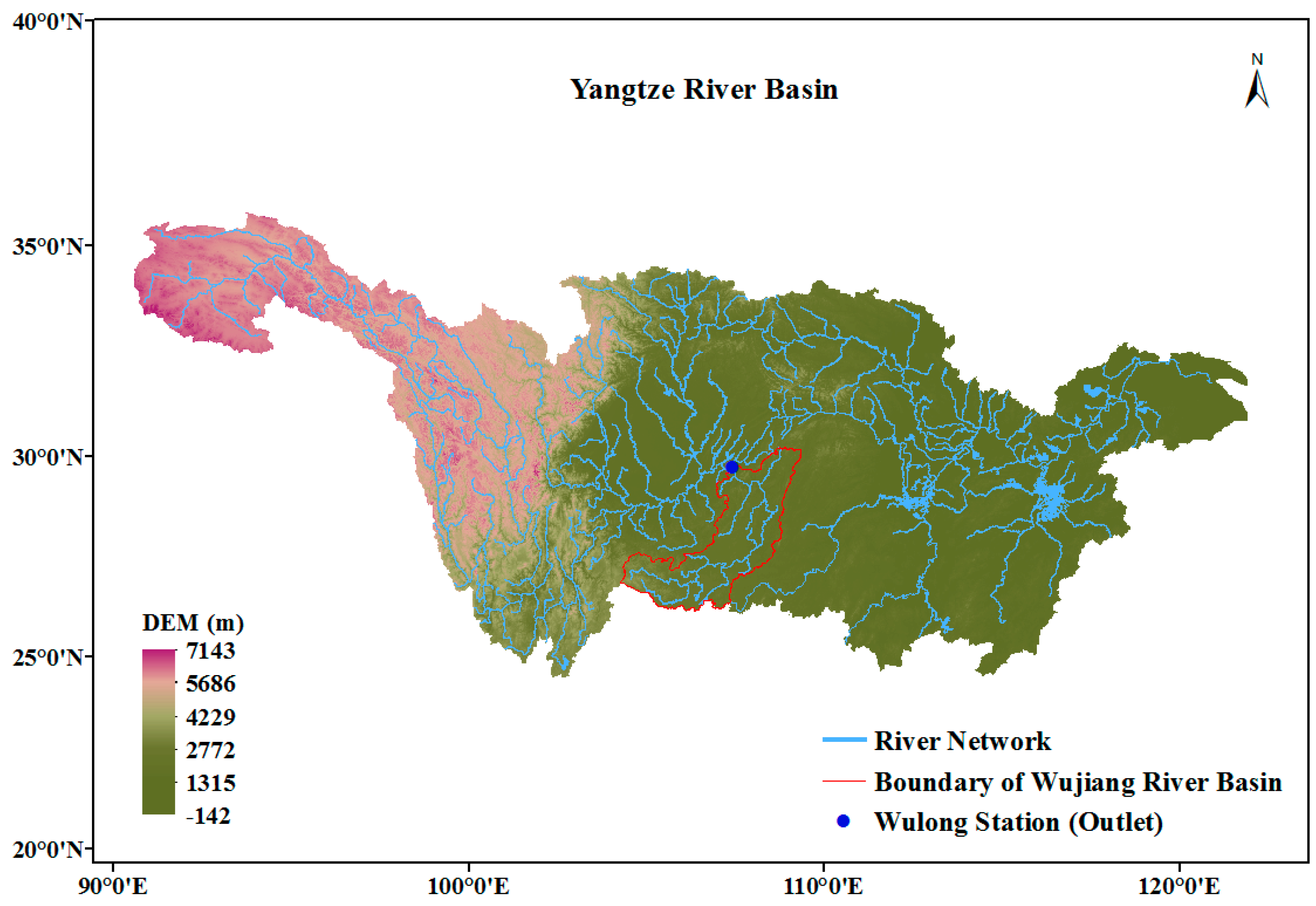
Figure 1. Geographical location of the Yangtze River basin. The upstream sub-basin, the Wujiang catchment, was used to model the hydrological effect of bias-corrected satellite precipitation estimates.
Remotesensing 11 01345 g001
Figure 2. Spatial distribution of averaged gridded daily precipitation analysis (GDPA) (a) before check, (b) after check with correction, and (c) of gauge intensities used in the optimal interpolation.
Remotesensing 11 01345 g002
Figure 3. Flowchart of the bias correction process used in the study.
Remotesensing 11 01345 g003
Figure 4. The schematic diagram of (a) transfer function of distribution mapping used in bias correction, and (b) the censored shifted change of parametric statistical distribution.
Remotesensing 11 01345 g004
Figure 5. Spatial distribution of average daily (a) ground gridded reference precipitation, GDPA at raw 0.5° spatial resolution, (b) GDPA resampled at 0.1° spatial resolution, (c) “Final” post-real-time satellite precipitation estimates, IMERG-F, (d) raw “Early” near-real-time satellite precipitation estimates, IMERG-E selected to bias correct in this study, (e) difference (Diff.) between IMERG-F and resampled GDPA, and (f) Diff. between IMERG-E and resampled GDPA.
Remotesensing 11 01345 g005
Figure 6. Scatter plot and histogram of parameter set used in traditional bias correction of mixed Bernoulli and gamma distributions (BerGam), taking the whole study period time window, i.e., the first scheme of screening time windows, as an example.
Remotesensing 11 01345 g006
Figure 7. Scatter plot and histogram of parameter set as well as the object function (Obj. F) value used in improved bias correction of CSMD, taking the whole study period time window, i.e., the first scheme of screening time windows, as an example. These parameters were estimated by a simulated annealing algorithm.
Remotesensing 11 01345 g007
Figure 8. Summary of four metrics in space over Yangtze River basin. (a) MAE, in which lower values indicate better performance; and (b) MD, mNSE, and KGE, in which higher values indicate better performance. BerGam and CSMD are the traditional and improved bias correction of distribution mapping respectively, while whole, mon, and MW denote three different time-window selection schemes, as discussed in Section 3.2, used to sample precipitation data for one routine. Thus BerGam–whole denotes the traditional BerGam approach implemented using the whole period time-window scheme. Similarly, the other five short names represent the combination of a specific approach and time window scheme.
Remotesensing 11 01345 g008
Figure 9. Quantile-Quantile plot (Q-Q plot) of the raw or corrected IMERG-E satellite precipitation and post-processed IMERG-F against ground reference GDPA precipitation over (a) the whole intensity range and (b) the extreme range. The threshold of extreme precipitation is set to the 97.5 percentile, than which precipitation is greater was selected as extreme values.
Remotesensing 11 01345 g009
Figure 10. Cumulative probability distribution (CDF) of all precipitation datasets used, including the raw and corrected satellite precipitation IMERG-E, the post-real-time IMERG-F and the ground reference precipitation GDPA. (a) Over all intensities of the precipitation series, and (b) over relatively high intensities of precipitation series with their corresponding CDF values of 0.91–1.
Remotesensing 11 01345 g010
Figure 11. Performance of two bias-correction approaches on satellite precipitation IMERG-E in a summer heavy rainfall event during 5 June 2017–2 July 2017. Values of Correlation Coefficient (CC) metric between the raw IMERG-E, bias-corrected IMERG-E, and IMERG-F against GDPA were displayed in the legend. To ensure the lines are clearly observed, only the monthly time window scheme in each bias correction approach (with best performance among three time-window schemes in each approach), i.e., BerGam_mon and CSMD_mon, was used to exhibit here.
Remotesensing 11 01345 g011
Figure 12. Performance of hydrological effect of bias-corrected satellite precipitation estimates IMERG-E, detected by streamflow simulated via lumped GR6J and distributed CREST models at the Wulong outlet of the Wujiang catchment.
Remotesensing 11 01345 g012
Table 1. Parameter information used in the lumped GR6J and distributed CREST models.
NameDescriptionRangeUnit
GR6JX1Production store capacity100–1400mm
X2Intercatchment exchange coefficient−4–4mm/d
X3Routing store capacity0–500mm
X4Unit hydrograph time constant0–10d
X5Intercatchment exchange threshold−4–4
X6Coefficient for emptying exponential store0–20mm
CRESTKsatSoil saturate hydraulic conductivity10–3000mm/d
WMMean water capacity80–200mm
BExponent of the variable infiltration curve0.05–1.5
IMImpervious area ratio0–0.2
KEFactor to convert the potential evapotranspiration (ET) to local actual ET0.1–1.5
coeMOverland runoff velocity coefficient1.0–150
expMOverland flow speed exponent0.1–2.0
coeRMultiplier used to convert overland flow speed to channel flow speed1.0–3.0
coeSMultiplier used to convert overland flow speed to interflow speed0.001–1.0
KSOverland reservoir discharge parameter0–1.0
KIInterflow reservoir discharge parameter0–1.0
Table 2. Metrics used to evaluate the performance of corrected precipitation series against the reference data GDPA.
Statistical MetricPerfect MatchEquation
PrecipitationMean absolute error (MAE) a0 M A E = i = 1 n | X s i m , i X o b s , i | n
Modified index of agreement (MD) b1 M D = 1 i = 1 n | X s i m , i X o b s , i | j i = 1 n ( | X s i m , i X ¯ o b s | + | X o b s , i X ¯ o b s | ) j
Modified Nash–Sutcliffe efficiency (mNSE)1 m N S E = = 1 i = 1 n | X s i m , i X o b s , i | j i = 1 n ( | X o b s , i X ¯ o b s | ) j
Kling-Gupta efficiency (KGE) c1 K G E = 1 E D
E D = [ s r × ( r 1 ) ] 2 + [ s α × ( α 1 ) ] 2 + [ s β × ( β 1 ) ] 2
α = σ s σ o , β = μ s μ o
Correlation Coefficient (CC)1 C C = [ i = 1 n ( X s i m , i X ¯ s i m ) ( X o b s , i X ¯ o b s ) ] 2 i = 1 n ( X s i m , i X ¯ s i m ) 2 i = 1 n ( X o b s , i X ¯ o b s ) 2
StreamflowNash–Sutcliffe efficiency (NSE) d1 N S E = 1 i = 1 n ( Y s i m , i Y o b s , i ) 2 i = 1 n ( Y ¯ o b s , i Y o b s , i ) 2
Correlation Coefficient (r)1 r = [ i = 1 n ( Y s i m , i Y ¯ s i m ) ( Y o b s , i Y ¯ o b s ) ] 2 i = 1 n ( Y s i m , i Y ¯ s i m ) 2 i = 1 n ( Y o b s , i Y ¯ o b s ) 2
Relative deviation (RD)0 R D = 1 n i = 1 n Y s i m , i Y o b s , i Y o b s , i
a: X s i m , i is the ith raw/corrected IMERG-E, X o b s , i is the ith reference GDPA, n is the length of the series, b: j is set to 1 in MD and the following mNSE, c: ED is the Euclidian distance from the ideal point in the scaled space, s r , s α , and s β are used for adjusting the emphasis on different components, r is the Pearson product–moment correlation coefficient, and μ and σ denote the mean and standard deviation respectively, d: Y s i m , i and Y o b s , i represent the simulated and observed streamflow, respectively. A bar over X or Y denotes the average value.
Table 3. Performance of streamflow simulation driven by the raw IMERG-E, bias-corrected IMERG-E, post-real-time IMERG-F and ground reference GDPA.
GR6JCREST
CalibrationValidationCalibrationValidation
NSErRD (%)NSErRD (%)NSErRD (%)NSErRD (%)
BerGam_whole0.620.79−0.700.300.66−17.300.620.79−4.220.680.86−9.83
BerGam_mon0.490.70−1.70−0.150.05−20.100.570.76−4.420.660.83−9.06
BerGam_MW0.470.690.300.400.63−0.500.580.77−4.260.670.83−6.54
CSMD_whole0.510.72−0.500.510.74−5.800.450.73−10.860.620.86−20.11
CSMD_mon0.560.750.100.350.68−16.600.580.78−6.380.690.86−12.74
CSMD_MW0.560.750.400.440.71−11.300.590.77−3.390.740.87−10.08
IMERG-E0.450.680.800.480.692.800.520.72−6.140.740.87−9.77
IMERG-F0.560.750.010.540.74−4.400.580.78−5.810.700.87−12.40
GDPA0.620.79−1.400.450.71−10.500.560.80−13.720.170.79−45.91
Shadowed numbers highlighted the first three best (for NSE and r metrics is highest, for RD is the least absolute value) values in that column.