Article

A Sub-Regional Extraction Method of Common Mode Components from IGS and CMONOC Stations in China

1
GNSS Research Center, Wuhan University, Wuhan 430079, Hubei, China
2
Collaborative Innovation Center for Geospatial Information Technology, Wuhan 430079, Hubei, China
*
Author to whom correspondence should be addressed.
Remote Sens. 2019, 11(11), 1389; https://doi.org/10.3390/rs11111389
Submission received: 26 March 2019 / Revised: 31 May 2019 / Accepted: 3 June 2019 / Published: 11 June 2019

Abstract

:
There is always a need to extract more accurate regional common mode component (CMC) series from coordinate time series of Global Positioning System (GPS) stations, which would be of great benefit to describe the deformation features of the Earth’s surface with more reliability. For this purpose, this paper combines all 11 International Global Navigation Satellite System (GNSS) Service (IGS) stations in China with over 70 stations selected from the Crustal Movement Observation Network of China (CMONOC) to compute CMC series of IGS stations by using a principal component analysis (PCA) method under cases of one whole region and eight sub-regions. The comparison results show that the percentage of first-order principal component (PC1) in North, East and Up components increase by 10.8%, 16.1% and 25.1%, respectively, after dividing the whole China region into eight sub-regions. Meanwhile, Root Mean Square (RMS) reduction rates of residual series that have removed CMC also improve obviously after partitioning. In addition, we compute displacements of these IGS stations caused by environmental loadings (including atmospheric pressure loading, non-tidal oceanic loading and hydrological loading) to analyze their contributions to the non-linear variation in GPS coordinate time series. The comparison result shows that the method we raise, PCA filtering in sub-regions, performs better than the environmental loading corrections (ELCs) in improving the signal-to-noise ratio (SNR) of GPS coordinate time series. This paper raises new criteria for selecting appropriate CMONOC stations around IGS stations when computing sub-regional CMC, involving three criteria of interstation distance, geology and self-condition of stations themselves. According to experiments, these criteria are implemental and effective in selecting suitable stations, by which to extract sub-regional CMC with higher accuracy.

Graphical Abstract

1. Introduction

The continuously operating GNSS reference stations established by the International GNSS Service (IGS) have accumulated a huge amount of GNSS data for over 20 years. The results from these data, coordinate time series of IGS stations, are constantly getting more accurate, accompanied by the gradual improvement of GNSS technology, data-processing methods and error correction models. Topics, such as the global or regional observation of crust deformation and regional fault slips have significant scientific value and practical meaning [1,2,3,4,5,6]. However, the coordinate time series of GPS stations have various influential factors, including one related to time and space is called common mode error (CME) [7,8]. CME series have obvious periodic terms that are probably caused by some geophysical signals [9,10]. Therefore, we use the term “common mode component” (CMC) in this paper instead.
Effective extraction of CMC is quite beneficial in improving the accuracy of coordinate time series, quantifying the station displacement caused by geophysical signals and accurately describing the features of regional earth surface deformation. As a result, recent years have seen CMC become a heated research topic [9,10,11,12,13,14,15,16,17,18,19]. Jiang et al. [20] analyzed 29 stations in the Chinese CORS network and extracted the CMC series by using a PCA method. After filtering CMC from the original coordinate time series, they estimated the velocity and its accuracy of each station. Tian and Shen [15] put forward a correlation-weighted stacking filtering method to remove CMC. This method takes the correlation coefficients of the coordinate components (North, East and Up) among the stations as the weighs in filtering, then the root mean square (RMS) value reduced effectively. Besides, it is available in both large-scale and small-scale GPS networks. Ma et al. [16] employed three kinds of spatial filtering approaches: stacking, PCA and Karhunen-Loeve Expansion (KLE) to extract CMC from stations in the Antarctic Peninsula. The results showed that PCA is an efficient filtering method with the highest accuracy. Zhu et al. [18] calculated the CMC of CMONOC stations through correlation weighted stacking filtering method. Then they quantified the geophysical signals that induced CMC, including environmental loading and thermal expansion. The results announced that environmental loading is one of the main sources of CMC in the vertical component of stations, while the impact of thermal expansion is not as obvious as the former.
Through continuous exploration in recent years, theoretical CMC research has matured, whereas there are still questions worth to discussing further. For example, when we compute the CMC of all the stations in a whole region, the CMC of the sub-regions would be easily regarded as the local individual feature and hence be neglected. This would then lead to decreasing CMC extraction accuracy and inaccurate cognition about the motion features of GPS stations. In addition, according to the existing research results [11,18,21,22], the scale of the research region has direct influence to extracting CMC, so what are the specific characteristics of such influence in China region? Does it have some useful and feasible instructions for the regional CMC extraction mode that this paper proposes? We will explore these topics next.

2. Data and Methodology

2.1. Data

2.1.1. GPS Coordinate Time Series

The data that this paper uses to calculate the CMC of IGS stations in China region is mainly from Scripps Orbit and Permanent Array Center (SOPAC), one of IGS data analysis centers, and from China Earthquake Administration (CEA) that provides CMONOC data. Table 1 shows the related information about their products that we use in this paper. SOPAC products are from the address “ftp://garner.ucsd.edu/pub/timeseries/measures” which contains “raw” series that include outliers, “cleaned” series that has excluded outliers and “detrend” series that has removed linear trend. CMONOC products are acquired from “ftp://ftp.cgps.ac.cn/products/position/gamit/” which includes coordinate time series of 260 CMONOC stations that spread evenly throughout China. They are also divided into “raw” and “detrend” series.
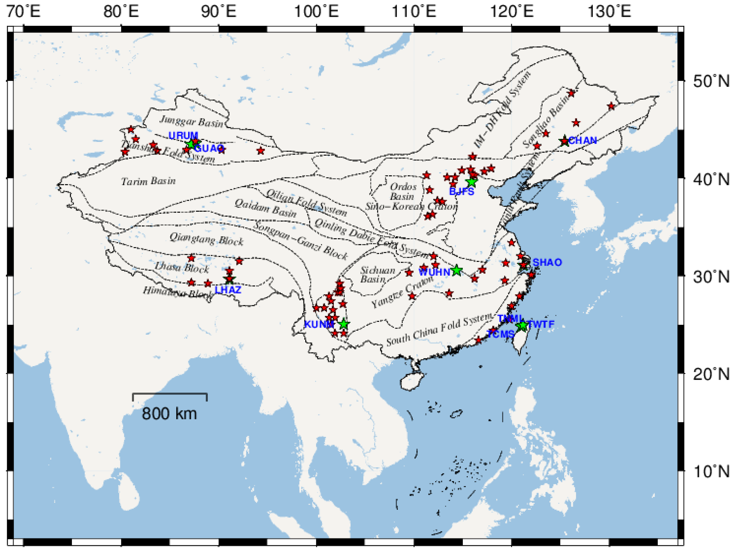
The daily loosely constraint solutions of these CMONOC stations are processed by the software GAMIT10.4. The detailed processing strategy emerges in the manual whose address is “ftp://ftp.cgps.ac.cn/doc/processing_manual.pdf”. Figure 1 shows all the IGS and CMONOC stations in China. The data that this paper uses is the “cleaned” series of 11 IGS stations and “detrend” series of over 70 selected CMONOC stations.

2.1.2. Environmental Loading Data

The mass redistribution of atmosphere, ocean and terrestrial water reserves can cause changes in the Earth’s surface mass loading, thus leading to surface deformation [23,24,25]. This is called environmental loading deformation. Surface loading models (SLM) can be established based on geophysical observations and Earth models to estimate surface displacements caused by environmental loadings.
This paper estimates the displacement of IGS stations caused by environmental loading based on the surface loading products provided by GFZ [26]. GFZ provides global surface elastic deformation data in grids form, including atmospheric pressure loading (NTAL), non-tidal oceanic loading (NTOL) and hydrological loading (HYDL), with a spatial resolution of 0.5° × 0.5°. The temporal resolution is 3 h for NTAL and NTOL data, and 24 h for HYDL data. The input data GFZ calculates NTAL, NTOL and HYDL are surface pressure data from European Centre for Medium-Range Weather Forecasts (ECMWF), Max Planck Institute Ocean Model (MPIOM, [27]) and land surface discharge model (LSDM, [28]). Based on the environmental loading products (netCDF files) of GFZ, we adopt a bicubic interpolation to interpolate certain station locations and then to compute the environmental loading series of each CMONOC station. In order to unify the temporal resolution of these environmental loading displacement series, NTAL and NTOL displacement series take the average every six epochs to get the daily time series. Then we add these three loadings together to acquire the sum environmental loading (SUML) of 11 IGS stations in China. The surface elastic deformation data used takes the Center of Earth’s Figure (CF) as the reference frame [29].

2.2. Methodology

At present, the popular method for CMC extraction is spatiotemporal filtering, which includes regional stacking [7,21,30], PCA [10,31,32] and KLE [9]. The CMC series is contained in the residual time series of stations, so when we get the original coordinate time series, the first thing is always to acquire the residual series by removing the linear and periodic terms.

2.2.1. Acquisition of the Residual Time Series

The original coordinate time series of GPS stations consists of a linear trend, periodic terms (annual and semi-annual), offsets and noises, so the mathematical model that reflects the displacement at coordinate components (North, East and Up) can be expressed as follows [33,34]:
v ( t ) = x ( t ) [ x R + v ( t t R ) + j = 1 n b b j H ( t t j ) + k = 1 n A A k s i n ( ω k t + φ k ) + k = 1 n L a k l o g ( 1 + ( t t k ) / T k ) ) ]
where xR and tR are the reference coordinate and epoch; t are epochs of GPS time series; v means linear velocity; H(t) is the Heaviside step function and used to model offsets with amplitudes bj; nb is the number of offsets and tj are epochs of these offsets; Ak, wk, φk are the amplitudes, angular velocities and initial phases of periodic signals, respectively; nA is the number of periodic signals, k = 1 for annual signal and k = 2 for semi-annual signal; nL is the number of logarithmic functions used to model post-seismic deformation; ak and Tk are two parameters of the logarithmic function; tk are the epochs of earthquakes that caused logarithmic displacement; v(t) is the residual series that represents the difference between the observations and the fitting values. It is also used for extracting CMC series.
For offsets contained in coordinate time series, firstly we remove some of them (including earthquakes and antenna/receiver changing) based on the epochs defined by CEA. Then we manually inspect the remaining offsets in stations one by one, as it is a better method to distinguish them [35]. If some large earthquakes near a station happened right in the same epochs, we assume that these offsets are probably caused by earthquakes and remove them in the GPS time series. Besides, a few station components have obvious post-seismic relaxations, and we use logarithmic functions to fit them. We use least squares fitting (LSF) method to calculate the linear trend, periodic terms and post-seismic relaxations in Equation (1), then we obtain the residual series of each station component. For outliers remaining in residual series, three-time interquartile range (3IQR) method is used for culling. After acquiring the residual series, then we extract CMC from them.

2.2.2. Principal Component Analysis

PCA is a popular approach to reduce the dimensionality of high-dimensional data. The principle is to transform the original data into a set of linearly independent components and then obtain the principal components (PCs) that represent the biggest contributors to the original data. In the application of GPS coordinate time series, PCA decomposes the residual series of GPS stations into PCs in the temporal domain and the corresponding eigenvectors in the spatial domain. Then the spatiotemporal variation of the GPS network can be expressed to the largest extent through the first several PCs.
For a regional GPS network with n stations that spanning m days, their residual coordinate time series compose a matrix:
X ( t i , x j )   ( i = 1 , 2 , , m ; j = 1 , 2 , , n )
B is the corresponding covariance matrix with elements that are defined as:
b i , j = 1 m 1 k = 1 m X ( t k , x i ) X ( t k , x j )
The symmetric matrix B can be decomposed as:
B = V Λ V T
where V T ( n × n ) , formed by eigenvectors, is a matrix with orthonormal rows; Λ is a diagonal matrix composed by non-zero eigenvalues of matrix B; generally in real GPS data, matrix B is full in rank, which means r = n . The eigenvalues and eigenvectors of matrix B can be written as ( λ 1 , v 1 ) , ( λ 2 , v 2 ) , , ( λ n , v n ) . v 1 , v 2 , , v n is a set of orthonormal bases that help to expand X ( t i , x j ) :
X ( t i , x j ) = k = 1 n a k ( t i ) v k ( x j )
where a k ( t ) is the k-th PC and can be derived by:
a k ( t i ) = j = 1 n X ( t i , x j ) v k ( x j )
where v k ( x ) is the eigenvector of matrix B. PCs represent the temporal variations and the eigenvectors represent the spatial responses to the PCs.
The decomposition result of PCA is arranged in descending order, which means the first-order principal component (PC1) always retains the largest amount of information about the regional GPS network. PC1 reflects the common temporal characteristics of the whole network, while the high-order PCs are usually related to local or individual site effects. The eigenvectors of these PCs, however, reflect the spatial distribution of the corresponding temporal change. As a result, we calculate CMC by:
ε ( t i , x j ) = k = 1 p a k ( t i ) v k ( x j )
where p refers to the number of PCs that remains to be ascertained in real data processing.
PCA has the advantage of simplifying questions and making them intuitive because it converts a question from high dimensions to lower dimensions. Besides, it obtains the features of the CMC spatiotemporal distribution completely through the original data itself, unlike the regional stacking filtering method that firstly supposes that the spatial distribution of CMC is even. Due to these merits, we employ PCA to compute the CMC in the research region.

3. CMC Extraction

In this section, we use PCA to extract CMC of IGS stations in two modes. The first extraction mode is one whole extraction from all IGS stations in China, a direct and most popular method. Another extraction mode that this paper proposes is eight sub-regional extractions, taking near CMONOC stations and tectonic units into consideration. Our purpose is to gain a CMC series with more accuracy.

3.1. One Extraction from all IGS Stations

Figure 1 shows all eleven IGS stations in China. The longest baseline is TWTF to GUAO, with 3654 km while the shortest is TNML to TCMS, only 8 m. The average length of these baselines is 2016 km, so the GPS network is medium-scale [22]. Next, we use PCA to extract CMC from all IGS stations in China, in order to analyze the amount of CMC in this medium-scale network.
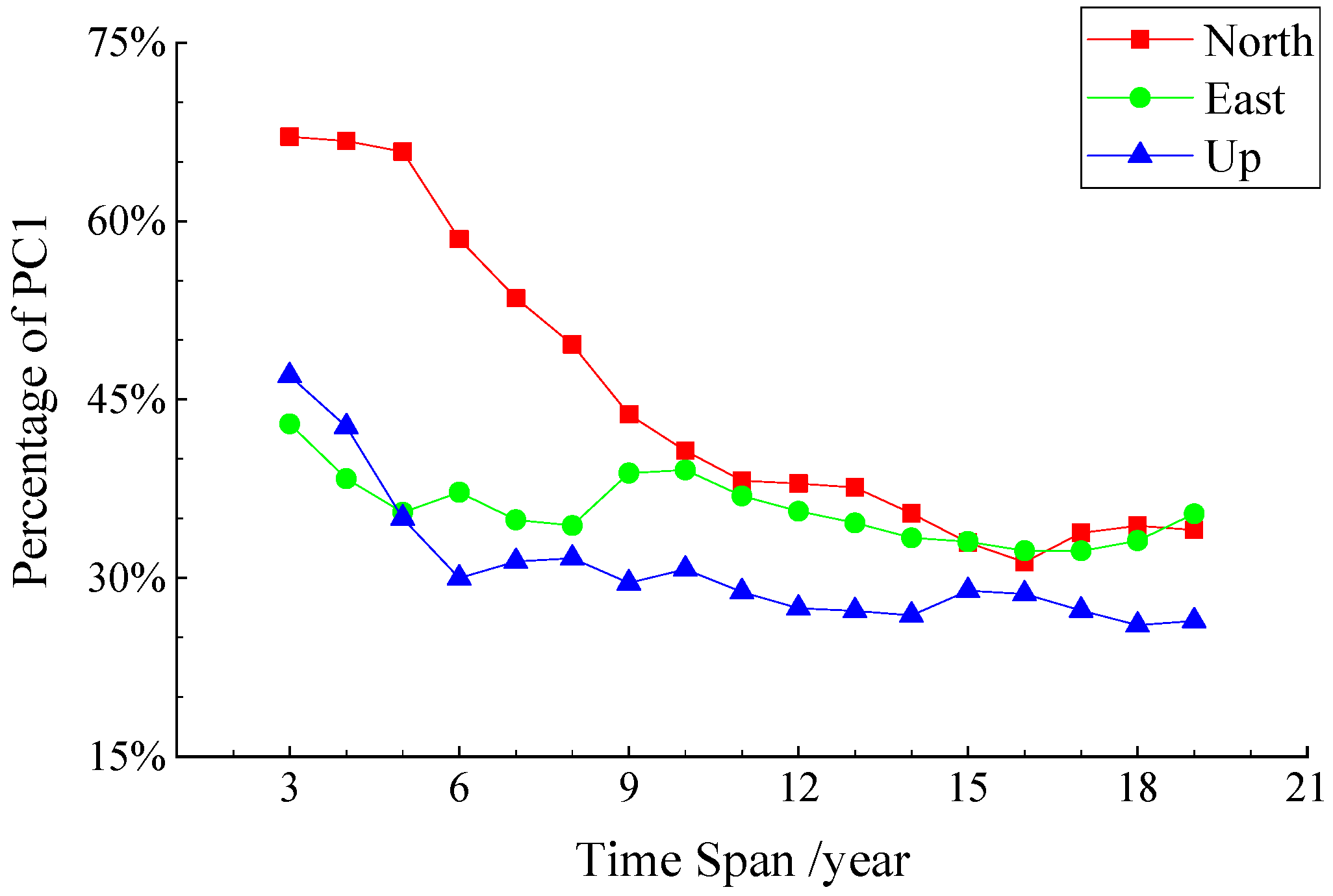
Figure 2 illustrates the effect of different time spans of the coordinate time series on the percentage of PC1 when uniformly extracting the CMC of the IGS station in China. In general, the length of the coordinate time series is inversely proportional to the percentage of PC1. The longer the time span is, the smaller the percentage of PC1. This can be understood as the longer the coordinate time series accumulated by each station, the less significant the common components in the residual series. Specifically, when the time series span is less than 10 years, the percentage of PC1 varies greatly with different time spans. When the time span is longer than 10 years, it gradually becomes stable. The percentages of PC1 in North and East components are about 34%, and about 26% in Up component.
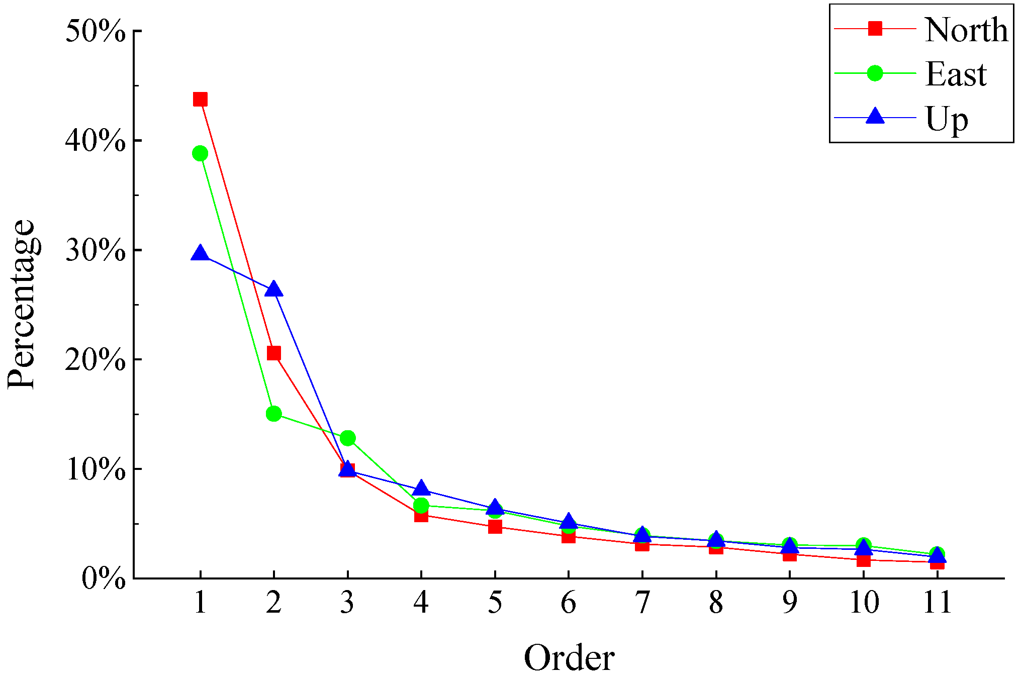
For the coordinate time series of a nine years’ span (2010–2019), Figure 3 shows the percentage of all the 11 PCs in North, East and Up component, which is also the contribution rate of each PC to the residual time series. Table 2 gives information about normalized eigenvectors of top three PCs. They are unitless values calculated through the eigenvalue of one station dividing the largest eigenvalue among these stations.
For identifying the number of PC used for computing CMC, we can choose it both from eigenvalues and eigenvectors. According to the treatment of Dong et al. [9], we regard the component as PC if most sites (more than 50%) have significant normalized responses (larger than 0.25). From Figure 3, we know that the contribution percentage of PC1 to residual series in North, East and Up is 43.8%, 38.8% and 29.6% respectively. Table 2 shows that the normalized eigenvectors of PC1 are over 0.25 on each component of more than 50% sites, while the normalized eigenvectors of PC2 meet the above demand in North component but fail in East and Up. Consequently, the CMC on North is PC1 and PC2, while the CMC on East and Up components is PC1 only.
Considering the fact that the contribution percentage of PC1 that represents regional common deformation is small, the CMC of all IGS stations in China region probably fails to be extracted accurately. From the above equations, CMC extraction is influenced by the number of GPS stations and distances among them. Therefore, it is highly necessary to combine some CMONOC stations to extract CMC of these IGS stations in higher accuracy. When deciding the available CMONOC stations, this paper takes two factors into account, the distance away from an IGS station and division of tectonic units. As the region size has a direct influence on CMC extraction, we should ascertain the appropriate region size and study the features of such influence in China.

3.2. Influence of Region Size on CMC Extraction

When exploring the influence of region size on CMC extraction, we choose one satisfactory experimental region. Given the fact that Northeast Block of China is the most stable among all blocks in China, without an obvious interior fault zones [36], it proves to be the most suitable research region. Moreover, most CMONOC stations in Northeast Block have similar monument types and geological features, which helps to approximately regard the distance as the unique variable that influences the accuracy of CMC extraction.
The spatial distribution of IGS and CMONOC stations in Northeast Block of China is shown in Figure 4. When carrying out this experiment, we employ a strategy that takes CHAN, an IGS station, as the region center and the radius is 300, 400, 500, 600, 700, 800, 900 and 1050 km respectively. A series of concentric circles contain 19 CMONOC stations that locate in northeastern three provinces and eastern part of Inner Mongolia. The information of the total 20 stations is given in Table 3. These CMONOC stations were constructed at different times. The earliest two stations, SUIY and HLAR, were built up in 1999 (the first-stage CMONOC project, CMONOC-I). The latest station is JLYJ that was established in 2011 (the second-stage CMONOC project, CMONOC-II). Corresponding to Section 3.1, this section also uses the coordinate time series with a time span of 9 years (2010–2019) as the research object.
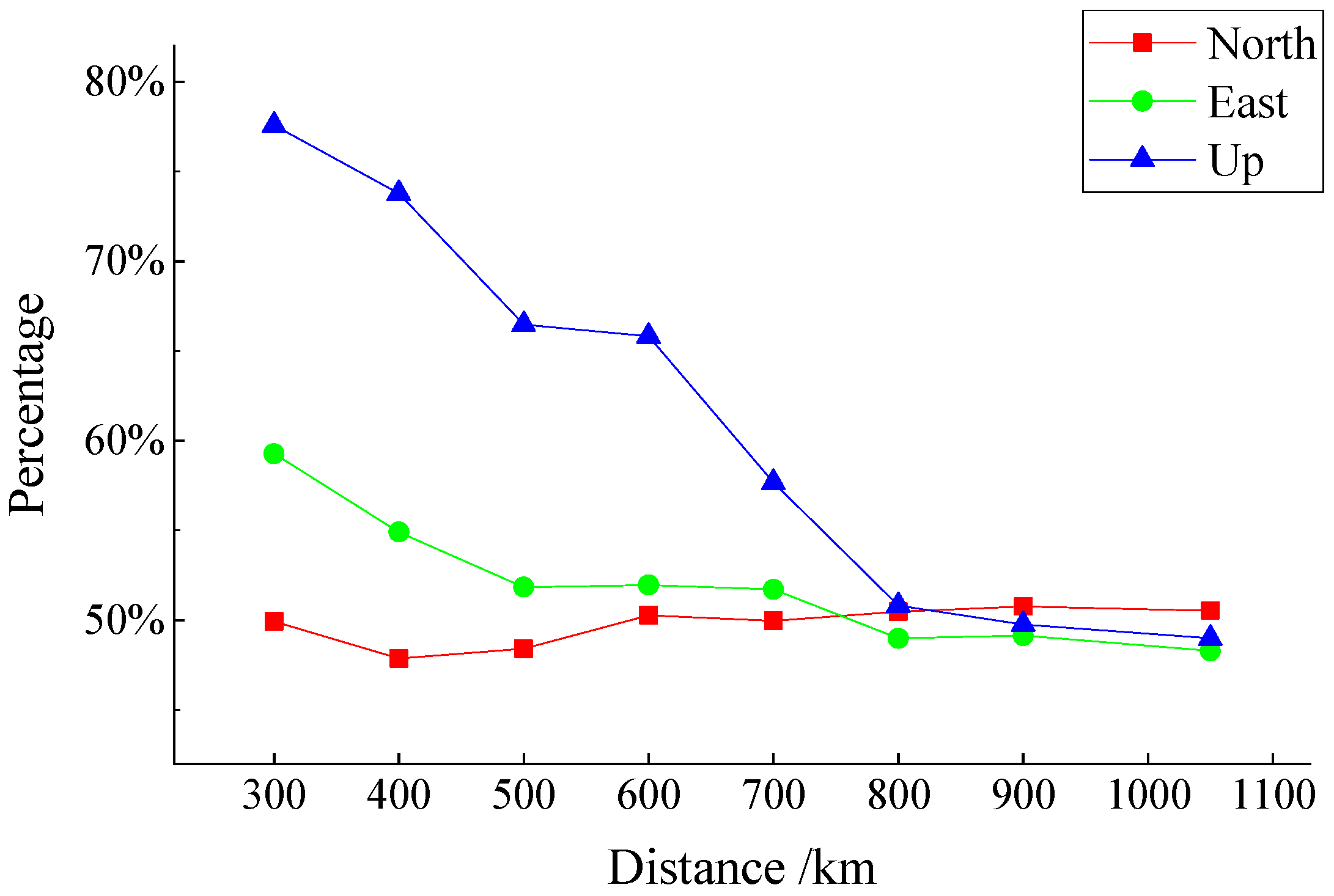
We use PCA to decompose the residual series of stations that locate in circles with different radiuses. Figure 5 demonstrates the relation between region size and the contribution percentage of PC1 in extracting CMC. In this region, the contribution percentage of PC1 in horizontal components (North and East) remains steady as the region size increases gradually. In the East, it has a slight decrease from 300 km to 1050 km, while in the North it is nearly unchanged and arrives 50% slower. However, the contribution percentage of PC1 in vertical component (Up) has a strong relation with region size. It drops significantly along with the increase of distance, from 78% to only 49%. Furthermore, we notice that the change trend of the Up component falls dramatically between 600 km and 700 km, with the figure going from 66% to 58%. In summary, CMC can be extracted accurately in a region of 600 km, and the contribution percentages of PC1 in North, East and Up components are more than 50%.

3.3. Sub-Regional Extractions Considering Tectonic Units

It is necessary to combine the CMONOC stations around IGS stations in order to acquire more accurate CMC from IGS stations in the China region. Above we discussed the influence of the region size on CMC extraction, and this may provide a criterion to choose suitable CMONOC stations. However, the Northeast Block is the most stable throughout China and the established criterion may not necessarily hold for other blocks. In cases where the region is less stable, we suggest that there is a strong need for another criterion, namely geology, to further restrain selecting stations. In this paper, we raise second-class tectonic units as the geology criterion [37,38] because CMC can be extracted more accurately in a relatively small-sized and stable region according to Section 3.2. What’s more, the self-condition of stations should also be combined together with these selection criteria, such as the completeness of the coordinate time series, time span, and whether there is some short-term drastic land subsidence or some unexplained offsets.
Criteria for selecting CMONOC stations are protocoled in this paper as follows. First, interstation distance criterion: The distance between one CMONOC station and IGS station does not exceed 600 km. Second, geology criterion: CMONOC stations and IGS station are in the same second-class tectonic unit. Third, self-condition criterion: It means that coordinate time series have a time span of over 5 years with 60% completeness, and meanwhile without apparent tectonic movements.
According to these criteria, some stations are discarded. They include XZCY and XZGZ whose distances to LHAZ are more than 600 km in the Lhasa Sub-block. TJBH and TJWQ in Tianjin are also abandoned where there is drastic land subsidence because of groundwater exploitation. There are also some stations with unexplained offsets, such as SXCZ and NMBT that are discarded. After the selecting process, we get the sub-regional division of IGS stations as shown in Figure 6. Table 4 gives information about the eight divided sub-regions.
The construction time of IGS stations in China is generally earlier than that of the CMONOC stations, and even the running time of CMONOC stations are various. It makes the coordinate time series of these stations with different starting epoch and time span. Considering that most CMONOC-II stations were established in 2010, similarly, we use the coordinate time series with a time span of nine years (2010–2019) when computing CMC. In addition, the starting epochs of CMONOC stations in each region are firstly arranged in a ranked order, then we choose the middle epoch as the starting epoch in PCA filtering process. In this way, the number of stations that participate in the CMC calculation in each region is over half of the total stations.
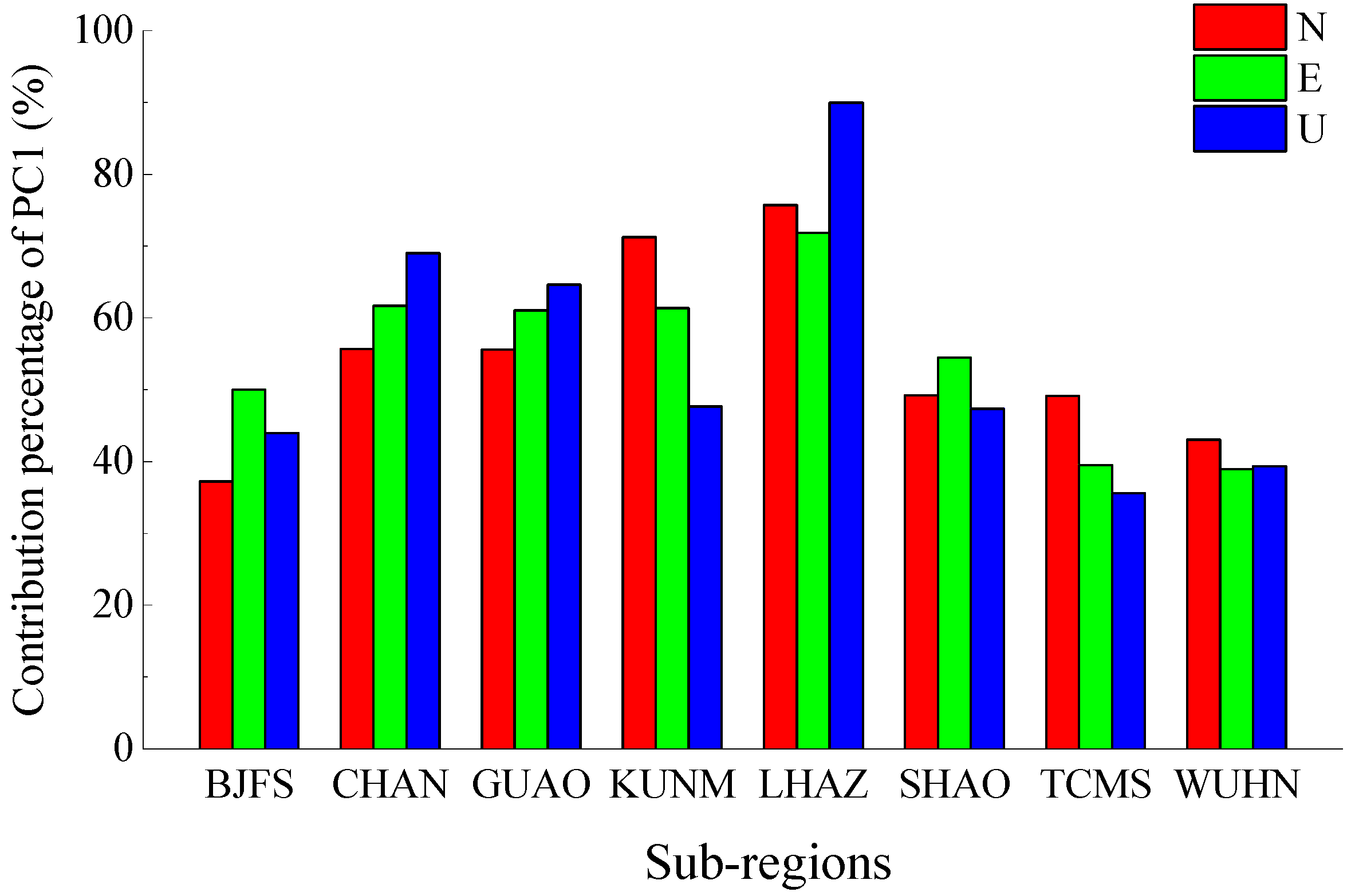
We use PCA to decompose the residual series of the stations in each sub-region, and contribution percentage of PC1 is shown in Figure 7. After analyzing the eigenvalues and normalized eigenvectors in all sub-regions, we define PC1 as CMC in each sub-region. From Figure 7, apart from a few coordinate components, the contribution percentages of PC1 are over 40% in most components. Especially in Lhasa Sub-block, the indicators on three coordinate components are all over 70%, representing that most of CMC there can be extracted precisely by PCA filtering. The average values on the N, E and U component are 54.6%, 54.9% and 54.7%, which increases by 10.8%, 16.1% and 25.1% respectively, compared with the results of mode 1. From this, we know that this indicator, contribution percentages of PC1, can be an important assessment criterion of CMC extraction.

3.4. Comparison of Two CMC Extraction Modes

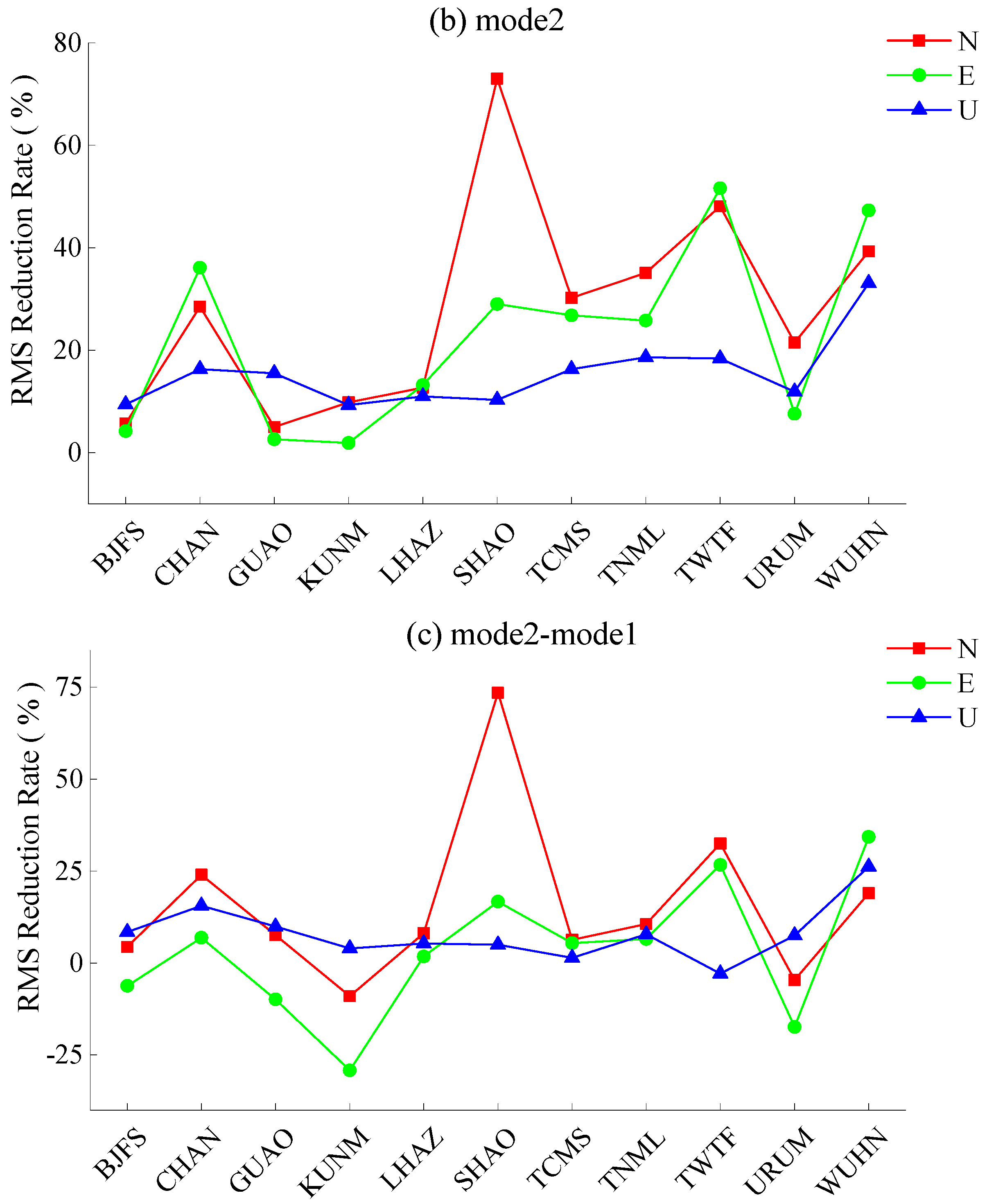
In addition to the contribution percentage of PC1 as an indicator, there is another indicator which can be used to evaluate the effect of CMC extraction under the above two modes. This indicator is RMS reduction rate of residual series before and after PCA filtering (shown in Equation (7)). Figure 8 shows RMS reduction rate of residual time series in Chinese IGS stations under cases of mode 1, mode 2, and the difference between the two modes:
R M S reduce = R M S b e f o r e R M S a f t e r R M S b e f o r e
Among the 33 coordinate components of 11 IGS stations, RMS reduction rates of 31 coordinate components after PCA filtering under mode 1 are positive values (shown in Figure 8a), and RMS reduction rates of all 33 coordinate components after PCA filtering under mode 2 are positive (shown in Figure 8b). The results show that PCA filtering is indeed an effective method to improve the signal-to-noise ratio (SNR) of GPS coordinate time series. Meanwhile, CMC extraction mode that proposed in this paper (mode 2) is more robust than overall filtering of an entire region (mode 1). Figure 8c shows the difference in RMS reduction rate for the two modes. There are 26 coordinate components (accounting for 78.8%) have positive values in the difference of RMS reduction rate, indicating that mode 2 is a more effective filtering method on most coordinate components.

4. Relevant Geophysical Signals

The nonlinear variations of GPS coordinate time series contain a variety of geophysical signals. Current research focuses are on the displacements of GPS stations under the impact of surface environmental loadings such as atmospheric pressure, oceanic tide and hydrology [19,39].
In this section, based on the grid data of loading deformation provided by GFZ, we adopt bicubic interpolation to calculate the displacement series at 11 IGS stations in China. Taking CHAN station as an example, Figure 9 shows the station displacement caused by NTAL, HYDL, NTOL and the sum of these displacements, SUML. In order to further explore the relation between environmental loading and CMC, and the source of CMC, we remove the annual and semi-annual terms in Equation (1) to obtain the residual series, with the seasonal periodic term in them. Thus, it helps to study the characteristics of non-linear variations in GPS coordinate time series [33]. Using the same methods and steps as in the previous section, we get the CMC series in mode 2. These series contain significant seasonal periodic signals.
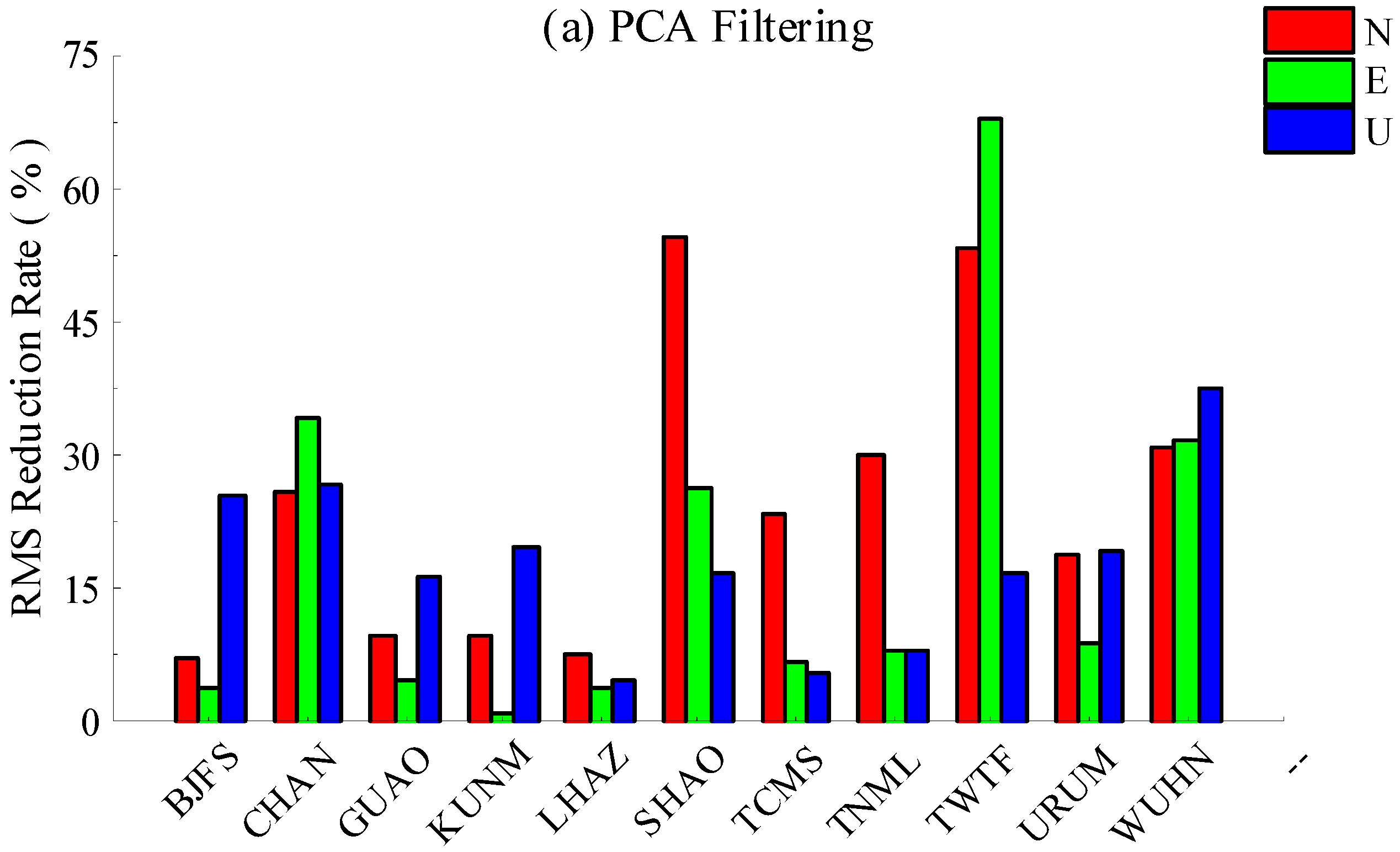
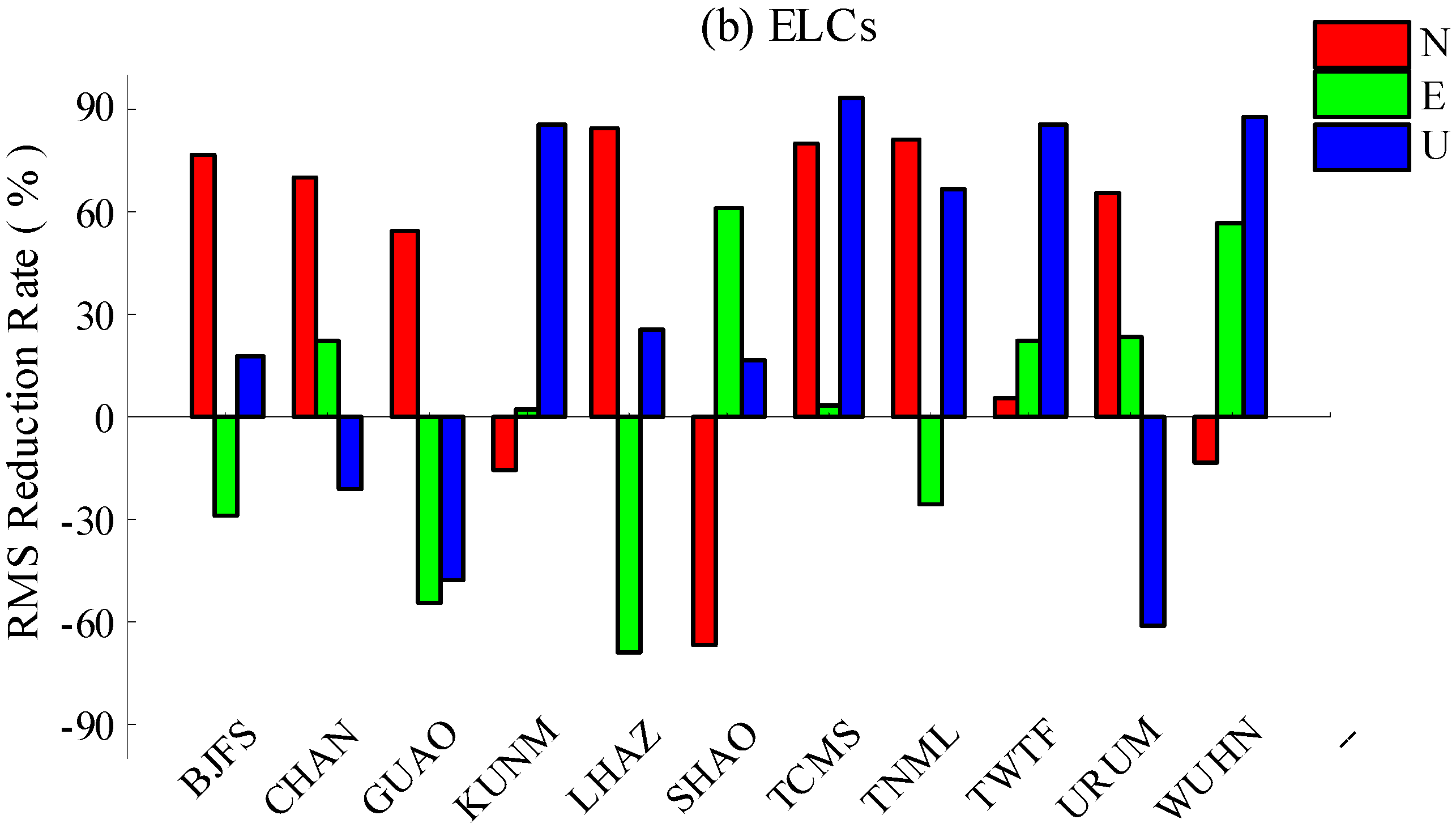
PCA filtering and environmental loading corrections (ELCs) are two commonly used methods for analyzing non-linear variations of GPS coordinate time series because both can effectively reduce SNR of GPS coordinate time series. In order to evaluate whether PCA filtering under mode 2 or ELCs is more effective for improving SNR of the GPS coordinate time series (especially in the vertical component), we calculate RMS reduction rate of residual series before and after PCA filtering and ELCs. The results are shown in Figure 10. As shown in Figure 10a, RMS reduction rates of all 33 coordinate components after PCA filtering are positive values, while 23 coordinate components after ELCs are positive, and RMS reduction rate of the remaining 30.3% of the coordinate components corrected by environmental loadings become larger (shown as some columns are below the horizontal axis in Figure 10b). This change in RMS reduction rates is consistent with the results from Jiang et al. [30]. Especially for the three vertical coordinate components shown in Figure 10b, which have negative RMS reduction rates. Given the fact that there is an apparent phase difference between the periodic terms of environmental loading displacement and GPS coordinate time series in vertical component, there is less RMS reduction rate for ELCs than PCA filtering. This reveals the high efficiency of PCA filtering under mode 2 that we demonstrate in this paper, and this PCA filtering under mode 2 is superior to ELCs in improving the SNR of the GPS coordinate time series.

5. Conclusions

Combining some selected CMONOC stations, we employ a PCA filtering method to compute regional CMC of IGS stations in China under two extraction modes, one whole extraction of all eleven IGS stations and eight sub-regional extractions combined with near CMONOC stations. The following conclusions may be drawn:
(1)
The average PC1 contribution percentage of eight sub-regions in North, East and Up components are 54.6%, 54.9% and 54.7%, which increase by 10.8%, 16.1% and 25.1%, respectively, compared with the result of one whole region. The regional CMC extracted in sub-regional mode are more significant, and RMS reduction rates on more coordinate components are positive values after CMC extraction. Moreover, the differences of RMS reduction rates are positive on 78.8% coordinate components, indicating that PCA filtering in a sub-regional mode is a more effective filtering method for most coordinate components. This will help to improve SNR in GPS coordinate time series, and thus to reveal the surface deformation characteristics of the IGS station more realistically and accurately.
(2)
Regional CMC is a spatiotemporal-dependent displacement series. It is affected by factors, such as the region size and time span of the coordinate time series. When the CMC of the IGS station in China is uniformly extracted, the length of the coordinate time series is inversely proportional to the percentage of PC1. The longer the time span is, the smaller the percentage of PC1. When the time series span is greater than 10 years, the percentage of PC1 in North and East components are about 34%, and about 26% in the Up component. In the Northeast Block of China, regional CMC of GPS stations can be extracted satisfactorily within the interstation distance of 600 km. The contribution percentages of PC1 in North, East and Up components are all over 50%, and along with the increase of region size, it does not change significantly in horizontal components but drops dramatically in the vertical direction.
(3)
This paper puts forward new criteria for selecting appropriate CMONOC stations near IGS stations when computing sub-regional CMC, including considerations of interstation distance, geology and self-condition of stations. Experimental results show that these criteria are implemental and effective in selecting suitable stations. PCA filtering with the above-mentioned criteria helps to improve the accuracy of coordinate time series of GPS stations, which is beneficial to reveal the deformation of the Earth surface.
(4)
PCA filtering and environmental loading corrections are two commonly used methods for analyzing non-linear variations of GPS coordinate time series. By comparison, we know that PCA filtering in sub-regional mode results in dramatic improvements of SNR in GPS coordinate time series. After ELCs, however, there are still 30.3% of the coordinate components with larger RMS reduction rates, probably because of the phase differences of the periodic terms between GPS coordinate time series and environmental loading displacements in the vertical components. Therefore, PCA filtering in sub-regional mode is superior to ELCs in improving the SNR of the GPS coordinate time series.

Author Contributions

Conceptualization, S.W., G.N. and J.L.; Data curation, S.W.; Formal analysis, S.W. and G.N.; Funding acquisition, S.W., G.N. and K.W.; Investigation, S.W., J.L., K.W. and H.L.; Methodology, S.W., J.L. and K.W.; Project administration, F.P.; Resources, G.N. and F.P.; Software, S.W., C.X., J.W. and X.R.; Supervision, G.N., J.L., C.X. and J.W.; Validation, C.X. and F.P.; Visualization, C.X.; Writing—original draft, S.W., G.N., J.W., H.L., F.P. and X.R.; Writing—review & editing, J.W., H.L. and X.R.

Funding

This research was funded by the National Key Basic Research Program of China, grant number 2013CB733205, and the National Natural Science Foundation of China, grant number 41074023.

Acknowledgments

The GPS coordinate time series of IGS stations in China are from the Scripps Orbit and Permanent Array Center (SOPAC). The GPS coordinate time series of CMONOC stations are from the China Earthquake Administration (CEA). Land surface environmental loading data comes from the German Research Centre For Geosciences (GFZ). After obtaining the CMC series, we used QOCA software from Prof. Dong Danan to verify the results. We express our sincere thanks to them all!

Conflicts of Interest

The authors declare no conflict of interest.

References

  1. Jiang, Z.S.; Liu, J.N. The method in establishing strain field and velocity field of crustal movement using least squares collocation. Chin. J. Geophys. 2010, 53, 380–389, (in Chinese with English abstract). [Google Scholar] [CrossRef]
  2. Liang, S.M.; Gan, W.J.; Shen, C.Z.; Xiao, G.R.; Liu, J.; Chen, W.T.; Ding, X.G.; Zhou, D.M. Three-dimensional velocity field of present-day crustal motion of the Tibetan Plateau derived from GPS measurements. J. Geophys. Res. Solid Earth 2013, 118, 5722–5732. [Google Scholar] [CrossRef]
  3. Kreemer, C.; Blewitt, G.; Klein, E.C. A geodetic plate motion and Global Strain Rate Model. Geochem. Geophys. Geosyst. 2014, 15, 3849–3889. [Google Scholar] [CrossRef]
  4. Wang, W.; Qiao, X.J.; Yang, S.M.; Wang, D.J. Present-day velocity field and block kinematics of Tibetan Plateau from GPS measurements. Geophys. J. Int. 2017, 208, 1088–1102. [Google Scholar] [CrossRef]
  5. Klos, A.; Gruszczynska, M.; Bos, M.; Boy, J.; Bogusz, J. Estimates of Vertical Velocity Errors for IGS ITRF2014 Stations by Applying the Improved Singular Spectrum Analysis Method and Environmental Loading Models. Pure Appl. Geophys. 2018, 175, 1823–1840. [Google Scholar] [CrossRef]
  6. Yuan, P.; Jiang, W.P.; Wang, K.H.; Sneeuw, N. Effects of Spatiotemporal Filtering on the Periodic Signals and Noise in the GPS Position Time Series of the Crustal Movement Observation Network of China. Remote Sens. 2018, 10, 1472. [Google Scholar] [CrossRef]
  7. Wdowinski, S.; Bock, Y.; Zhang, J.; Fang, P.; Genrich, J. Southern California permanent GPS geodetic array: Spatial filtering of daily positions for estimating coseismic and postseismic displacement induced by the 1992 Landers earthquake. J. Geophys. Res. Solid Earth 1997, 102, 18057–18070. [Google Scholar] [CrossRef]
  8. Johansson, J.M.; Davis, J.L.; Scherneck, H.G.; Milne, G.A.; Vermeer, M.; Mitrovica, J.X.; Bennett, R.A.; Jonsson, B.; Elgered, G.; Elósegui, P.; et al. Continuous GPS measurements of postglacial adjustment in Fennoscandia-1. Geodetic results. J. Geophys. Res. Solid Earth 2002, 107, ETG 3-1–ETG 3-27. [Google Scholar] [CrossRef]
  9. Dong, D.; Fang, P.; Bock, Y.; Webb, F.; Prawirodirdjo, L.; Kedar, S.; Jamason, P. Spatiotemporal filtering using principal component analysis and Karhunen—Loeve expansion approaches for regional GPS network analysis. J. Geophys. Res. Solid Earth 2006, 111, 1581–1600. [Google Scholar] [CrossRef]
  10. Yuan, L.; Ding, X.; Chen, W.; Guo, Z.H.; Chen, S.B.; Hong, B.S.; Zhou, J.T. Characteristics of daily position time series from the Hong Kong GPS fiducial network. Chin. J. Geophys. 2008, 51, 1372–1384, (in Chinese with English abstract). [Google Scholar] [CrossRef]
  11. Márquez-Azúa, B.; DeMets, C. Crustal velocity field of Mexico from continuous GPS measurements, 1993 to June 2001: Implications for the neotectonics of Mexico. J. Geophys. Res. Solid Earth 2003, 108, 149–169. [Google Scholar] [CrossRef]
  12. Serpelloni, E.; Faccenna, C.; Spada, G.; Dong, D.; Williams, S.D.P. Vertical GPS ground motion rates in the Euro-Mediterranean region: New evidence of velocity gradients at different spatial scales along the Nubia-Eurasia plate boundary. J. Geophys. Res. Solid Earth 2013, 118, 6003–6024. [Google Scholar] [CrossRef] [Green Version]
  13. Shen, Y.Z.; Li, W.W.; Xu, G.C.; Li, B.F. Spatiotemporal filtering of regional GNSS network’s position time series with missing data using principle component analysis. J. Geod. 2014, 88, 1–12. [Google Scholar] [CrossRef]
  14. He, X.X.; Hua, X.H.; Yu, K.G.; Xuan, W.; Lu, T.D.; Zhang, W.; Chen, X. Accuracy enhancement of GPS time series using principal component analysis and block spatial filtering. Adv. Space Res. 2015, 60, 1316–1327. [Google Scholar] [CrossRef]
  15. Tian, Y.F.; Shen, Z.K. Extracting the regional common-mode component of GPS station position time series from dense continuous network. J. Geophys. Res. Solid Earth 2016, 121, 1080–1096. [Google Scholar] [CrossRef]
  16. Ma, C.; Li, F.; Zhang, S.K.; Lei, J.T.; E, D.C.; Hao, W.F.; Zhang, Q.C. The coordinate time series analysis of continuous GPS stations in the Antarctic Peninsula with consideration of common mode error. Chin. J. Geophys. 2016, 59, 2783–2795, (in Chinese with English abstract). [Google Scholar]
  17. Ming, F.; Yang, Y.X.; Zeng, A.M.; Zhao, B. Spatiotemporal filtering for regional GPS network in China using independent component analysis. J. Geod. 2017, 91, 419–440. [Google Scholar] [CrossRef]
  18. Zhu, Z.H.; Zhou, X.H.; Deng, L.S.; Wang, K.H.; Zhou, B.Y. Quantitative Analysis of Geophysical Sources of Common Mode Component in CMONOC GPS Coordinate Time Series. Adv. Space Res. 2017, 60, 2896–2909. [Google Scholar] [CrossRef]
  19. Yuan, P.; Li, Z.; Jiang, W.P.; Ma, Y.F.; Chen, W.; Sneeuw, N. Influences of Environmental Loading Corrections on the Nonlinear Variations and Velocity Uncertainties for the Reprocessed Global Positioning System Height Time Series of the Crustal Movement Observation Network of China. Remote Sens. 2018, 10, 958. [Google Scholar] [CrossRef]
  20. Jiang, Z.H.; Zhang, P.; Bei, J.Z.; Liu, L.F. Velocity estimation on the colored noise properties of CORS network in China based on the CGCS2000 frame. Acta Geod. Cartogr. Sin. 2010, 39, 355–363, (in Chinese with English abstract). [Google Scholar]
  21. Williams, S.D.P.; Bock, Y.; Fang, P.; Jamason, P.; Nikolaidis, R.M.; Prawirodirdjo, L.; Miller, M.; Johnson, D.J. Error analysis of continuous GPS position time series. J. Geophys. Res. 2004, 109, B03412. [Google Scholar] [CrossRef]
  22. Tian, Y.F. Study on Intermediate- and long-term Errors in GPS Position Time Series. Ph.D. Thesis, Institute of Geology, China Earthquake Administration, Beijing, China, 2011. [Google Scholar]
  23. Farrell, W.E. Deformation of the Earth by surface loads. Rev. Geophys. 1972, 10, 761–797. [Google Scholar] [CrossRef]
  24. Van Dam, T.; Wahr, J.M. Displacements of the Earth’s surface due to atmospheric loading: Effects on gravity and baseline measurements. J. Geophys. Res. Solid Earth 1987, 92, 1281–1286. [Google Scholar] [CrossRef]
  25. Van Dam, T.; Böhm, J. Loading Effects and Reference Frames. In Encyclopedia of Geodesy; Grafarend, E., Ed.; Springer: Basel, Switzerland, 2016; pp. 1–5. ISBN 978-3-319-02370-0. [Google Scholar]
  26. Dill, R.; Dobslaw, H. Numerical simulations of global-scale high-resolution hydrological crustal deformations. J. Geophys. Res. Solid Earth 2013, 118, 5008–5017. [Google Scholar] [CrossRef]
  27. Marsland, S.J.; Haak, H.; Jungclaus, J.H.; Latif, M.; Röske, F. The Max-Planck-Institute global ocean/sea ice model with orthogonal curvilinear coordinates. Ocean Model. 2003, 5, 91–127. [Google Scholar] [CrossRef] [Green Version]
  28. Dill, R. Hydrological Model LSDM for Operational Earth Rotation and Gravity Field Variations; Scientific Technical Report STR08/09; GFZ: Potsdam, Germany, 2008. [Google Scholar]
  29. Blewitt, G. Self-consistency in reference frames, geocenter definition, and surface loading of the solid Earth. J. Geophys. Res. Solid Earth 2003, 108, B2. [Google Scholar] [CrossRef]
  30. Jiang, W.P.; Xia, C.Y.; Li, Z.; Guo, Q.Y.; Zhang, S.Q. Analysis of environmental loading effects on regional GPS coordinate time series. Acta Geod. Cartogr. Sin. 2014, 43, 1217–1223, (in Chinese with English abstract). [Google Scholar]
  31. Li, F.; Ma, C.; Zhang, S.K.; Lei, J.T.; Hao, W.F.; Zhang, Q.C.; Li, W.H. Noise analysis of the coordinate time series of the continuous GPS stations and deformation patterns in the Antarctic Peninsula. Chin. J. Geophys. 2016, 59, 2402–2412, (in Chinese with English abstract). [Google Scholar]
  32. Jackson, D.A.; Chen, Y. Robust principal component analysis and outlier detection with ecological data. Environmetrics 2004, 15, 129–139. [Google Scholar] [CrossRef]
  33. Bevis, M.; Brown, A. Trajectory models and reference frames for crustal motion geodesy. J. Geod. 2014, 88, 283–311. [Google Scholar] [CrossRef] [Green Version]
  34. Nikolaidis, R. Observation of Geodetic and Seismic Deformation with the Global Positioning System. Ph.D. Thesis, University of California, San Diego, CA, USA, 2002. [Google Scholar]
  35. Gazeaux, J. Detecting offsets in GPS time series: First results from the detection of offsets in GPS experiment. J. Geophys. Res. Solid Earth 2013, 118, 2397–2407. [Google Scholar] [CrossRef] [Green Version]
  36. Wang, X.Y.; Zhu, W.Y.; Fu, Y.; You, Z.X.; Wang, Q.; Cheng, Z.Y.; Ren, J.W. Present-time crustal deformation in China and surrounding regions by GPS. Chin. J. Geophys. 2002, 45, 198–209, (in Chinese with English abstract). [Google Scholar] [CrossRef]
  37. Liu, X.; Li, T.D.; Geng, S.F.; You, G.Q. Geotectonic division of China and some related problems. Geol. Bull. China 2012, 31, 1024–1034, (in Chinese with English abstract). [Google Scholar]
  38. Liu, X.; You, G.Q. Tectonic regional subdivision of China in the light of plate theory. Geol. China 2015, 42, 1–17, (in Chinese with English abstract). [Google Scholar]
  39. Jiang, W.P.; Li, Z.; Liu, H.F.; Zhao, Q. Cause analysis of the non-linear variation of the IGS reference station coordinate time series inside China. Chin. J. Geophys. 2013, 56, 2228–2237, (in Chinese with English abstract). [Google Scholar]
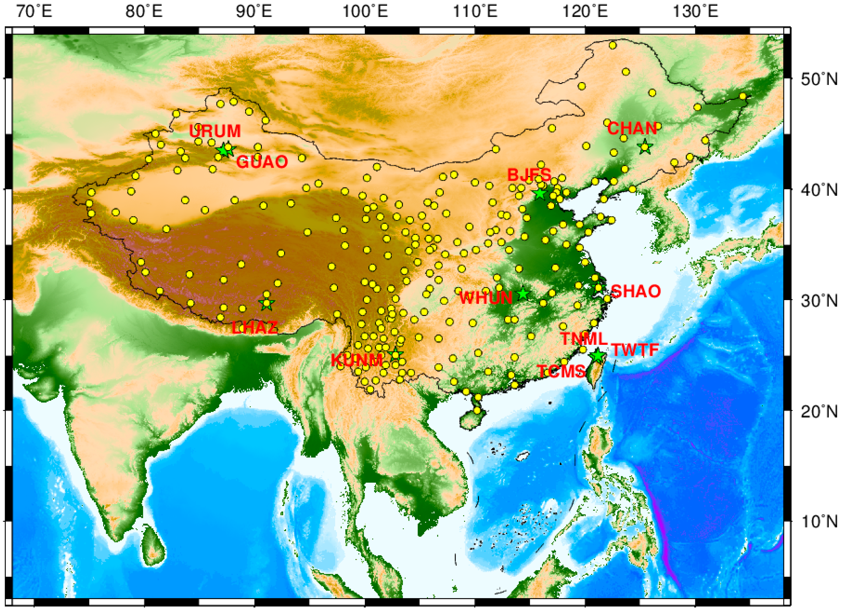
Figure 1. Distribution of IGS and CMONOC stations in China where all the eleven IGS stations are marked in red bold figures.
Remotesensing 11 01389 g001
Figure 2. Percentages of the first-order principal component when extracting CMC of IGS stations in China with different time spans.
Remotesensing 11 01389 g002
Figure 3. Percentage of the eigenvalue of each principal component to the total eigenvalue.
Remotesensing 11 01389 g003
Figure 4. Distribution of IGS and CMONOC stations in Northeast Block of China.
Remotesensing 11 01389 g004
Figure 5. The relationship between region size and the percentage of first-order principal component eigenvalues in extracting CMC (Northeast Block of China).
Remotesensing 11 01389 g005
Figure 6. Distribution of eight divided sub-areas according to IGS stations and their surrounding CMONOC stations that are chosen by the criteria proposed in this paper.
Remotesensing 11 01389 g006
Figure 7. Contribution percentage of PC1 in eight sub-regions. The column “TCMS” shows the corresponding percentage in the district contains all three IGS stations in Taiwan. Similarly, “GUAO” stands for the region where GUAO and URUM stations locate.
Remotesensing 11 01389 g007
Figure 8. RMS reduction rate of residual time series in Chinese IGS stations. (a) shows the RMS reduction rate of residual time series obtained from mode1, and (b) shows the RMS reduction rate of residual time series obtained from mode2. (c) shows the difference between (a,b). Note that the scales of the vertical axis in these figures are different from each other.
Remotesensing 11 01389 g008aRemotesensing 11 01389 g008b
Figure 9. Displacements on CHAN station caused by geophysical signals, including atmospheric loading (NTAL), hydrological loading (HYDL), non-tidal oceanic loading (NTOL) and their sum (SUML). Note that the scale of the vertical axis in (c) is smaller than (a,b,d) The displacements caused by environmental loadings in vertical component (Up) are much bigger than that in horizontal components (North and East). Among these three loadings, NTAL contributes the most to SUML; the second contributor is HYDL; and NTOL contributes the least to SUML. SUML represents obvious seasonal variations, and its amplitude can be up to 10 mm in some years.
Remotesensing 11 01389 g009aRemotesensing 11 01389 g009b
Figure 10. RMS reduction rate before and after PCA filtering (a) and environmental loading corrections (b) in the residual time series of IGS stations in China area.
Remotesensing 11 01389 g010aRemotesensing 11 01389 g010b
Table 1. Introduction of the original coordinate time series of IGS stations in China.
StationLatitude/°Longitude/°Session/yearTime Span/YearMonument/Bedrock Type
BJFS39.60861115.892221999.8041–2018.894519.1concrete/weathered sedimentary
CHAN43.79050125.443302004.9385–2018.897314.0concrete/weathered sedimentary
GUAO43.4711087.177302002.4534–2016.200813.7reinforced concrete/metamorphic
URUM43.5900087.630001998.7685–2013.083614.3concrete/bedrock
KUNM25.02950102.797201999.7247–2018.897319.2concrete/sedimentary
LHAZ29.6572291.103891995.0233–2018.897323.9roof concrete/none
SHAO31.09944121.200282002.4781–2018.880816.4concrete/sedimentary
TCMS24.79778120.987222002.4781–2018.869916.4roof steel/sedimentary
TNML24.79800120.987302001.8562–2018.894517.0roof steel/sedimentary
TWTF24.95360121.164501998.8342–2018.894520.1roof steel/none
WHUN30.53139114.357221996.0669–2016.736320.7granite block/sedimentary
Table 2. Eigenvectors of the first three PCs from IGS stations in China.
StationNorthEastUp
p1p2p3p1p2p3p1p2p3
BJFS−0.160.900.320.73−0.350.631.00−0.11−0.26
CHAN−0.121.00−0.220.86−0.33−0.060.70−0.02−0.08
GUAO−0.030.631.000.78−0.61−0.400.49−0.191.00
KUNM0.56−0.210.930.76−0.86−0.100.84−0.61−0.20
LHAZ0.160.920.600.80−0.40−0.150.650.070.80
URUM0.88−0.470.300.500.051.000.81−0.29−0.34
SHAO0.830.53−0.581.001.00−0.290.770.92−0.30
TCMS0.820.40−0.650.960.97−0.340.760.80−0.21
TNML1.00−0.14−0.070.540.200.220.051.000.33
TWTF−0.260.89−0.480.95−0.47−0.280.53−0.840.00
WUHN0.730.370.180.840.430.450.73−0.020.16
Table 3. Introduction of IGS station (CHAN) and CMONOC stations in Northeast Block of China.
StationLatitude/°Longitude/°Session/YearDistance Away to CHAN/kmMonument Type
CHAN43.79069125.444202004.9385–2018.98220bedrock
HRBN45.70261126.620372003.0014–2018.9959231.973soil
NMAG43.30348122.627222010.4973–2018.9959233.983bedrock
JLCB42.41055128.105932010.6233–2018.9959265.425bedrock
LNSY41.82708123.579482010.5849–2018.9959266.143soil
JLYJ42.68296129.504512011.1959–2018.9959344.581soil
NMWL46.04064122.027282011.0068–2018.9959367.755bedrock
LNYK40.68354122.603042010.5685–2018.9959417.151bedrock
LNDD40.03162124.327252010.6068–2018.9959427.606bedrock
NMAL43.86335120.112912010.7877−2018.9959428.789bedrock
SUIY44.43334130.908071999.1630−2018.9959443.044granodiorite
LNHL40.68769120.851802010.8178−2018.9959512.057bedrock
HLHG47.35276130.235632011.0041−2018.9959544.274bedrock
HLWD48.67141126.136172010.6041−2018.9959544.990bedrock
LNJZ39.09181121.740112011.0041−2018.9959606.403bedrock
NMDW45.51310116.963032010.6041−2018.9959698.775bedrock
HLAR49.27049119.741262010.4973−2018.9959749.134bedrock
NMER50.57642123.727201999.1630−2018.9959765.064andesite
HLFY48.36699134.277152010.6507−2018.9959850.307bedrock
HLMH52.97508122.512722011.0151−2018.99591042.765bedrock
Note: The fifth column represents the distances of CMONOC stations to CHAN that are calculated by their spatial rectangular coordinates (ITRF2008 Framework, epoch 2017.001). The precision presented here is 1 m.
Table 4. Information of eight divided sub-regions when extracting CMC of IGS stations combining CMONOC stations. Note that GUAO and URUM are in the same sub-region, and three IGS stations in Taiwan (TCMS, TNML and TWTF) are in the same sub-region.
StationLocationSecond-Class Tectonic UnitsNumber of Near CMONOC StationsThe Farthest CMONOC Station/Distance
BJFSBeijingNorth China Block (craton)16SXLF/558 km
CHANChangchunSongliao Basin7HLWD/545 km
GUAOUrumchiTianshan Fold System9XJJJ/586 km
KUNMKunmingSichuan-Yunnan Rhombic Block15SCSM/467 km
LHAZLhasaLhasa Sub-block6XZNM/440 km
SHAOShanghaiYangtze Block (craton)7JXHK/500 km
TCMSHsinchuSouth China Orogenic Zone6ZJZS/592 km
TNMLHsinchuSouth China Orogenic Zone6ZJZS/592 km
TWTFTaoyuanSouth China Orogenic Zone6ZJZS/573 km
URUMUrumchiTianshan Fold System9XJZS/600 km
WHUNWuhanYangtze Block (craton)7HNMY/532 km