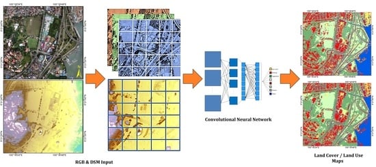
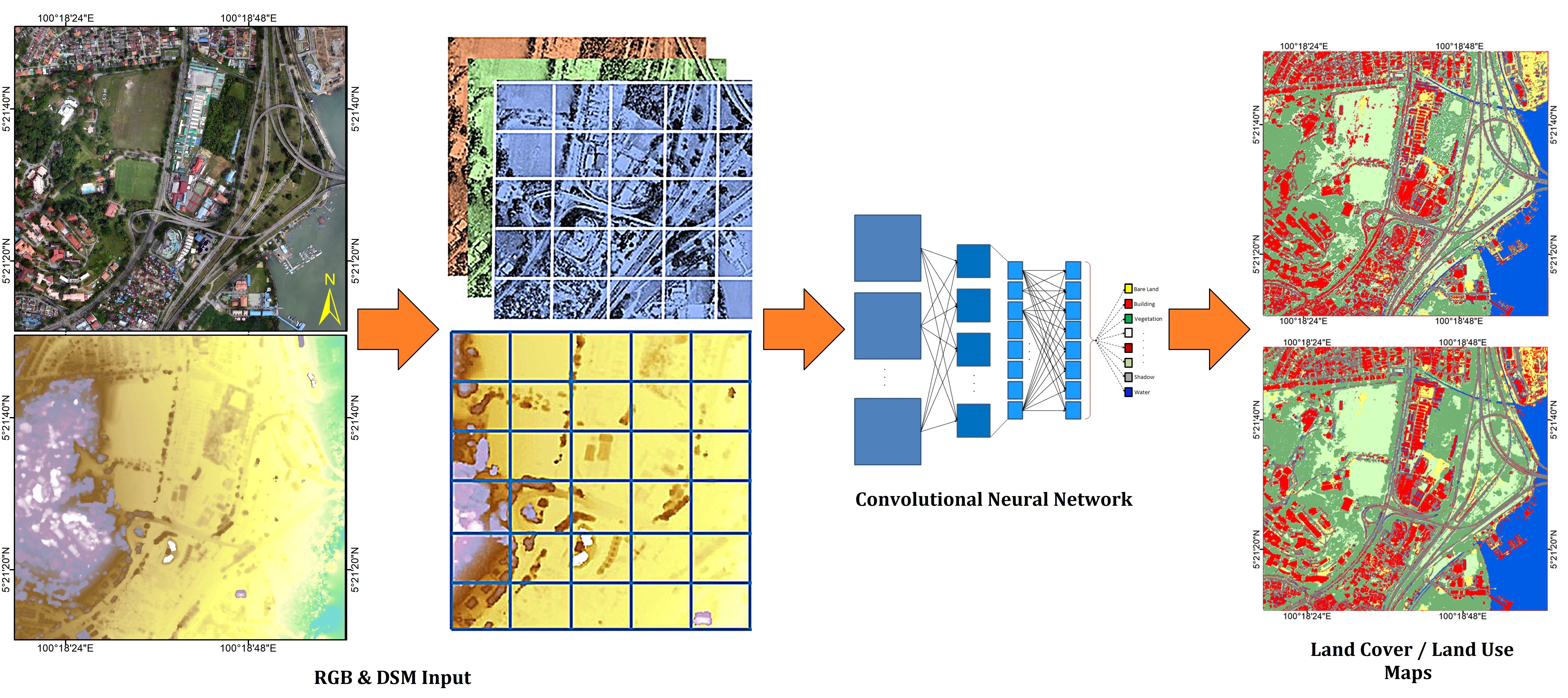
Land Cover Classification from fused DSM and UAV Images Using Convolutional Neural Networks


 ,
,  ,
,  ,
, 
Abstract
:
1. Introduction
2. Related Studies
3. Materials and Methods
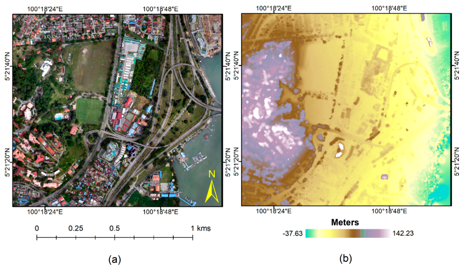
3.1. UAV Data Acquisition
3.2. Ground Truth Data
Training, Validation and Testing Set
3.3. Image Pre-Processing
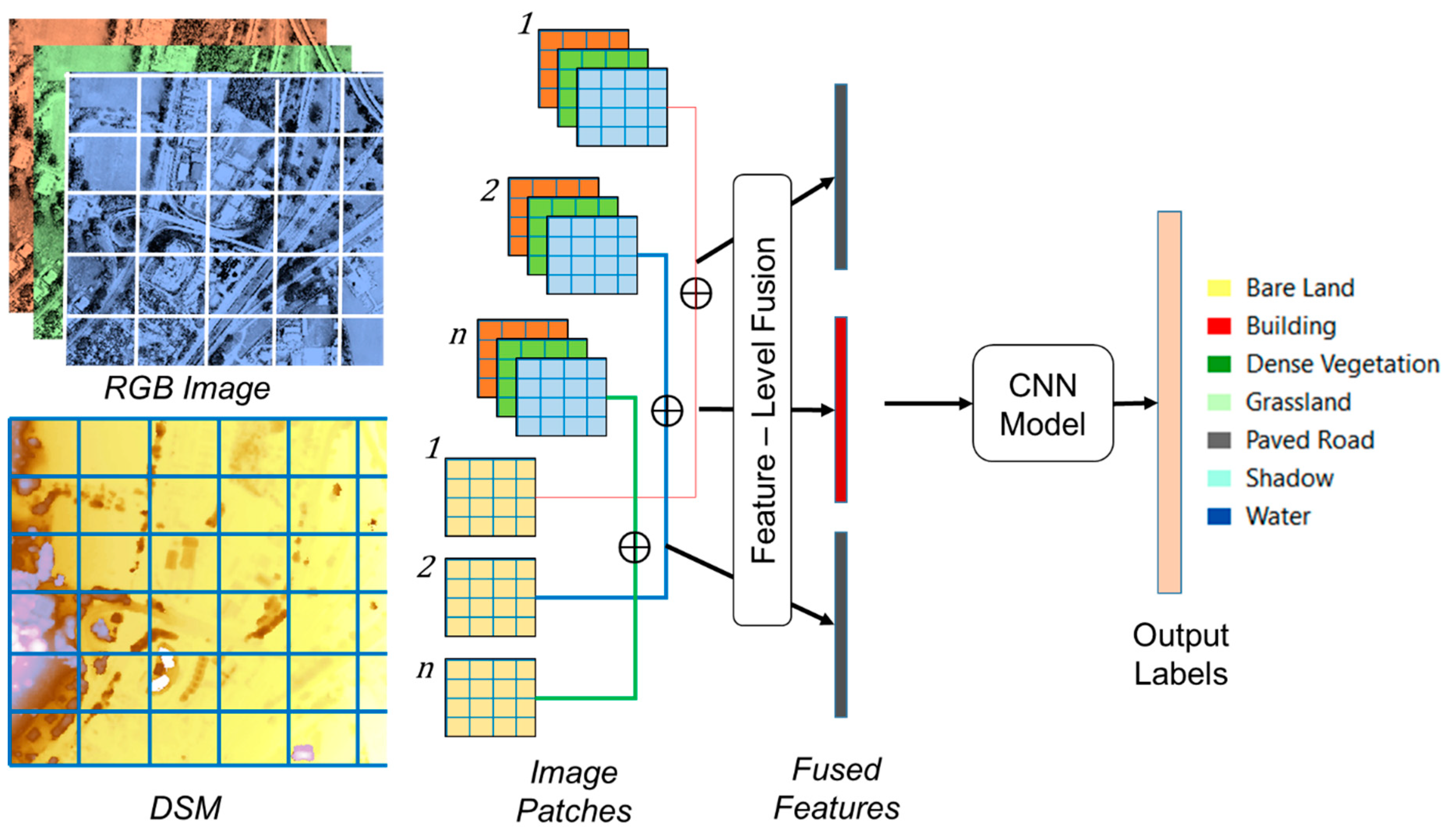
3.4. Methodology
Convolutional Neural Networks (CNNs)
3.5. Evaluation Metrics
4. Results
5. Discussion
6. Conclusions
Author Contributions
Funding
Acknowledgments
Conflicts of Interest
References
- Lucieer, A.; Robinson, S.A.; Turner, D. Using an Unmanned Aerial Vehicle (UAV) for Ultra-High Resolution Mapping of Antarctic Moss Beds. In Proceedings of the 2010 Australasian Remote Sensing Photogrammetry Conference, Alice Springs, NT, Australia, 14–16 September 2010; pp. 1–12. [Google Scholar]
- Al-Tahir, R.; Arthur, M. Unmanned Aerial Mapping Solution for Small Island Developing States. In Proceedings of the Global Geospatial Conference, Quebec City, QC, Canada, 14–17 May 2012; pp. 1–9. [Google Scholar]
- Kalantar, B.; Halin, A.A.; Al-Najjar, H.A.H.; Mansor, S.; van Genderen, J.L.; Shafri, H.Z.M.; Zand, M. A Framework for Multiple Moving Objects Detection in Aerial Videos. In Spatial Modeling in GIS and R for Earth and Environmental Sciences; Elsevier: Amsterdam, The Netherlands, 2019; pp. 573–588. [Google Scholar]
- Kalantar, B.; Mansor, S.B.; Halin, A.A.; Shafri, H.Z.M.; Zand, M. Multiple moving object detection from UAV videos using trajectories of matched regional adjacency graphs. IEEE Trans. Geosci. Remote Sens. 2017, 55, 5198–5213. [Google Scholar] [CrossRef]
- Lelong, C.; Burger, P.; Jubelin, G.; Roux, B.; Labbé, S.; Baret, F. Assessment of unmanned aerial vehicles imagery for quantitative monitoring of wheat crop in small plots. Sensors 2008, 8, 3557–3585. [Google Scholar] [CrossRef] [PubMed]
- Kalantar, B.; Mansor, S.B.; Sameen, M.I.; Pradhan, B.; Shafri, H.Z.M. Drone-based land-cover mapping using a fuzzy unordered rule induction algorithm integrated into object-based image analysis. Int. J. Remote Sens. 2017, 38, 2535–2556. [Google Scholar] [CrossRef]
- Kalantar, B.; Mansor, S.; Halin, A.A.; Ueda, N.; Shafri, H.Z.M.; Zand, M. A graph-based approach for moving objects detection from UAV videos. Image Signal Process. Remote Sens. XXIV 2018, 10789, 107891Y. [Google Scholar]
- Crommelinck, S.; Bennett, R.; Gerke, M.; Nex, F.; Yang, M.Y.; Vosselman, G. Review of automatic feature extraction from high-resolution optical sensor data for UAV-based cadastral mapping. Remote Sens. 2016, 8, 689. [Google Scholar] [CrossRef]
- Ma, L.; Li, M.; Ma, X.; Cheng, L.; Du, P.; Liu, Y. A review of supervised object-based land-cover image classification. ISPRS J. Photogramm. Remote Sens. 2017, 130, 277–293. [Google Scholar] [CrossRef]
- Liu, T.; Abd-Elrahman, A. An Object-Based Image Analysis Method for Enhancing Classification of Land Covers Using Fully Convolutional Networks and Multi-View Images of Small Unmanned Aerial System. Remote Sens. 2018, 10, 457. [Google Scholar] [CrossRef]
- Jahan, F.; Zhou, J.; Awrangjeb, M.; Gao, Y. Fusion of Hyperspectral and LiDAR Data Using Discriminant Correlation Analysis for Land Cover Classification. IEEE J. Sel. Top. Appl. Earth Obs. Remote Sens. 2018, 99, 1–13. [Google Scholar] [CrossRef]
- Gibril, M.B.A.; Bakar, S.A.; Yao, K.; Idrees, M.O.; Pradhan, B. Fusion of RADARSAT-2 and multispectral optical remote sensing data for LULC extraction in a tropical agricultural area. Geocarto Int. 2016, 1e14. [Google Scholar] [CrossRef]
- Gomez-Chova, L.; Tuia, D.; Moser, G.; Camps-Valls, G. Multimodal classification of remote sensing images: A review and future directions. Proc. IEEE 2015, 103, 1560–1584. [Google Scholar] [CrossRef]
- Marcos, D.; Volpi, M.; Kellenberger, B.; Tuia, D. Land cover mapping at very high resolution with rotation equivariant CNNs: Towards small yet accurate models. ISPRS J. Photogramm. Remote Sens. 2018, 145, 96–107. [Google Scholar] [CrossRef] [Green Version]
- Irwin, K.; Beaulne, D.; Braun, A.; Fotopoulos, G. Fusion of SAR, optical imagery and airborne LiDAR for surface water detection. Remote Sens. 2017, 9, 890. [Google Scholar] [CrossRef]
- Hartfield, K.A.; Landau, K.I.; van Leeuwen, W.J.D. Fusion of high resolution aerial multispectral and LiDAR data: Land cover in the context of urban mosquito habitat. Remote Sens. 2011, 3, 2364–2383. [Google Scholar] [CrossRef]
- Zhu, X.; Cai, F.; Tian, J.; Williams, T. Spatiotemporal Fusion of Multisource Remote Sensing Data: Literature Survey, Taxonomy, Principles, Applications, and Future Directions. Remote Sens. 2018, 10, 527. [Google Scholar] [Green Version]
- Sameen, M.I.; Pradhan, B.; Aziz, O.S. Classificationofveryhighresolutionaerialphotosusingspectral-spatial convolutional neural networks. J. Sens. 2018, 7195432. [Google Scholar]
- Wang, Y.; Wang, Z. A survey of recent work on fine-grained image classification techniques. J. Vis. Commun. Image Represent. 2019, 59, 210–214. [Google Scholar] [CrossRef]
- Feng, Q.; Liu, J.; Gong, J. UAV Remote sensing for urban vegetation mapping using Random Forest and texture analysis. Remote Sens. 2015, 7, 1074–1094. [Google Scholar] [CrossRef]
- Gevaert, C.M.; Persello, C.; Vosselman, G. Optimizing multiple kernel learning for the classification of UAV data. Remote Sens. 2016, 8, 1025. [Google Scholar] [CrossRef]
- Zhang, X.; Chen, G.; Wang, W.; Wang, Q.; Dai, F. Object-Based Land-Cover Supervised Classification for Very-High-Resolution UAV Images Using Stacked Denoising Autoencoders. IEEE J. Sel. Top. Appl. Earth Obs. Remote Sens. 2017, 10, 3373–3385. [Google Scholar] [CrossRef]
- Gibril, M.B.A.; Idrees, M.O.; Yao, K.; Shafri, H.Z.M. Integrative image segmentation optimization and machine learning approach for high quality land-use and land-cover mapping using multisource remote sensing data. J. Appl. Remote Sens. 2018, 12, 016036. [Google Scholar] [CrossRef]
- Gibril, M.B.A.; Shafri, H.Z.M.; Hamedianfar, A. New semi-automated mapping of asbestos cement roofs using rule-based object-based image analysis and Taguchi optimization technique from WorldView-2 images. Int. J. Remote Sens. 2017, 38, 467–491. [Google Scholar] [CrossRef]
- Liu, T.; Abd-Elrahman, A. Multi-view object-based classification of wetland land covers using unmanned aircraft system images. Remote Sens. Environ. 2018, 216, 122–138. [Google Scholar] [CrossRef]
- Liu, T.; Abd-Elrahman, A. Deep convolutional neural network training enrichment using multi-view object-based analysis of Unmanned Aerial systems imagery for wetlands classification. ISPRS J. Photogramm. Remote Sens. 2018, 139, 154–170. [Google Scholar] [CrossRef]
- Liu, T.; Abd-Elrahman, A.; Zare, A.; Dewitt, B.A.; Flory, L.; Smith, S.E. A fully learnable context-driven object-based model for mapping land cover using multi-view data from unmanned aircraft systems. Remote Sens. Environ. 2018, 216, 328–344. [Google Scholar] [CrossRef]
- Ma, L.; Fu, T.; Blaschke, T.; Li, M.; Tiede, D.; Zhou, Z.; Chen, D. Evaluation of Feature Selection Methods for Object-Based Land Cover Mapping of Unmanned Aerial Vehicle Imagery Using Random Forest and Support Vector Machine Classifiers. ISPRS Int. J. Geo Inf. 2017, 6, 51. [Google Scholar] [CrossRef]
- Bergado, J.R.A.; Persello, C.; Gevaert, C. A Deep Learning Approach to the Classification of Sub-Decimeter Resolution Aerial Images. In Proceedings of the IEEE International Geoscience and Remote Sensing Symposium, Beijing, China, 10–15 July 2016; pp. 1516–1519. [Google Scholar]
- Laliberte, A.S.; Goforth, M.A.; Steele, C.M.; Rango, A. Multispectral remote sensing from unmanned aircraft: Image processing workflows and applications for rangeland environments. Remote Sens. 2011, 3, 2529–2551. [Google Scholar] [CrossRef]
- Zhu, X.X.; Tuia, D.; Mou, L.; Xia, G.S.; Zhang, L.; Xu, F.; Fraundorfer, F. Deep Learning in Remote Sensing: A Comprehensive Review and List of Resources. IEEE Geosci. Remote Sens. Mag. 2017, 5, 8–36. [Google Scholar] [CrossRef] [Green Version]
- Guidici, D.; Clark, M.L. One-Dimensional convolutional neural network land-cover classification of multi-seasonal hyperspectral imagery in the San Francisco Bay Area, California. Remote Sens. 2017, 9, 629. [Google Scholar] [CrossRef]
- Zhang, P.; Ke, Y.; Zhang, Z.; Wang, M.; Li, P.; Zhang, S. Urban Land Use and Land Cover Classification Using Novel Deep Learning Models Based on High Spatial Resolution Satellite Imagery. Sensors 2018, 18, 3717. [Google Scholar] [CrossRef] [PubMed]
- Feng, Q.; Zhu, D.; Yang, J.; Li, B. Multisource Hyperspectral and LiDAR Data Fusion for Urban Land-Use Mapping based on a Modified Two-Branch Convolutional Neural Network. ISPRS Int. J. Geo Inf. 2019, 8, 28. [Google Scholar] [CrossRef]
- Kussul, N.; Lavreniuk, M.; Skakun, S.; Shelestov, A. Deep learning classification of land cover and crop types using remote sensing data. IEEE Geosci. Remote Sens. Lett. 2017, 14, 778–782. [Google Scholar] [CrossRef]
- Nahhas, F.H.; Shafri, H.Z.M.; Sameen, M.I.; Pradhan, B.; Mansor, S. Deep learning approach for building detection using liDAR-orthophoto fusion. J. Sens. 2018, 7212307. [Google Scholar] [CrossRef]
- Zhu, Y.; Newsam, S. Land Use Classification Using Convolutional Neural Networks Applied to Ground-level Images. In Proceedings of the 23rd SIGSPATIAL International Conference on Advances in Geographic Information Systems, Seattle, WA, USA, 3–6 November 2015; pp. 1–61. [Google Scholar]
- Liang, X.; Wang, X.; Lei, Z.; Liao, S.; Li, S.Z. Soft-Margin Softmax for Deep Classification. In International Conference on Neural Information Processing; Springer: Cham, Switzerland, 2017; pp. 413–421. [Google Scholar] [CrossRef]
- Kingma, D.; Ba, J. Adam: A method for stochastic optimization. arXiv 2014, arXiv:1412.6980. [Google Scholar]
- Ioffe, S.; Szegedy, C. Batch normalization: Accelerating deep network training by reducing internal covariate shift. arXiv 2015, arXiv:1502.03167. [Google Scholar]
- Jmour, N.; Zayen, S.; Abdelkrim, A. Convolutional Neural Networks for Image Classification. In Proceedings of the International Conference on Advanced Systems and Electric Technologies (IC_ASET), Hammamet, Tunisia, 22–25 March 2018; pp. 397–402.
- Mboga, N.; Persello, C.; Bergado, J.R.; Stein, A. Detection of Informal Settlements from VHR Images Using Convolutional Neural Networks. Remote Sens. 2017, 9, 1106. [Google Scholar] [CrossRef]
- Zang, W.; Lin, J.; Zhang, B.; Tao, H.; Wang, Z. Line-Based registration for UAV remote sensing imagery of wide-spanning river basin. In Proceedings of the 19th International Conference on Geoinformatics, Shanghai, China, 24–26 June 2011; pp. 1–4. [Google Scholar]
- Ramsey, E.W.; Jensen, J.R. Remote sensing of mangrove wetlands: Relating canopy spectra to site-specific data. Photogramm. Eng. Remote Sens. 1996, 62, 939. [Google Scholar]
- Congalton, R.G. A review of assessing the accuracy of classifications of remotely sensed data. Remote Sens. Environ. 1991, 37, 35–46. [Google Scholar] [CrossRef]
- Thoma, M. Analysis and optimization of convolutional neural network architectures. arXiv 2017, arXiv:1707.09725. [Google Scholar]
- Abd, H.A.A.R.; Alnajjar, H.A. Maximum Likelihood for Land-Use/Land-Cover Mapping and Change Detection Using Landsat Satellite Images: A Case Study South of Johor. Int. J. Comput. Eng. Res. (IJCER) 2013, 3, 26–33. [Google Scholar]
- Foody, G.M. Status of land cover classification accuracy assessment. Remote Sens. Environ. 2002, 80, 185–201. [Google Scholar] [CrossRef]
- Cheng, H.; Lian, D.; Gao, S.; Geng, Y. Evaluating Capability of Deep Neural Networks for Image Classification via Information Plane. In Proceedings of the European Conference on Computer Vision (ECCV), Munich, Germany, 8–14 September 2018; pp. 168–182. [Google Scholar]
- Tran, D.; Mac, H.; Tong, V.; Tran, H.A.; Nguyen, L.G. A LSTM based framework for handling multiclass imbalance in DGA botnet detection. Neurocomputing 2018, 275, 2401–2413. [Google Scholar] [CrossRef]


| Land Cover Class | Number of ROIs | Number of Pixels |
|---|---|---|
| Bare land | 27 | 1104 |
| Buildings | 129 | 3833 |
| Dense vegetation/trees | 53 | 1917 |
| Grassland | 47 | 3094 |
| Paved roads | 92 | 1343 |
| Shadows | 36 | 76 |
| Water bodies | 28 | 4183 |
| Model | ||||
|---|---|---|---|---|
| Training | CNN with DSM | 0.991 | 0.989 | 0.988 |
| CNN without DSM | 0.965 | 0.933 | 0.956 | |
| Testing | CNN with DSM | 0.980 | 0.970 | 0.976 |
| CNN without DSM | 0.968 | 0.952 | 0.961 |
| Class | CNN with DSM | CNN without DSM |
|---|---|---|
| Bare land | 0.996 | 0.981 |
| Buildings | 0.992 | 0.951 |
| Dense vegetation | 1.000 | 0.769 |
| Grassland | 0.956 | 0.946 |
| Paved roads | 0.990 | 0.995 |
| Shadows | 0.990 | 0.890 |
| Water bodies | 1.000 | 1.000 |
| Class | CNN with DSM | CNN without DSM |
|---|---|---|
| Bare land | 0.925 | 0.990 |
| Buildings | 0.983 | 0.979 |
| Dense vegetation | 0.966 | 0.923 |
| Grassland | 0.954 | 0.853 |
| Paved roads | 0.986 | 0.996 |
| Shadows | 0.978 | 0.923 |
| Water bodies | 0.999 | 0.999 |
| Class | CNN without DSM | CNN with DSM | ||||
|---|---|---|---|---|---|---|
| RecallMacro | PrecisionMacro | F1 ScoreMacro | RecallMacro | PrecisionMacro | F1 ScoreMacro | |
| Bare land | 0.976 | 0.998 | 0.987 | 0.959 | 1.00 | 0.979 |
| Buildings | 0.996 | 0.987 | 0.991 | 0.989 | 0.995 | 0.992 |
| Dense vegetation | 1.00 | 0.812 | 0.896 | 1.00 | 0.927 | 0.962 |
| Grassland | 0.872 | 1.00 | 0.931 | 0.954 | 1.00 | 0.976 |
| Paved roads | 0.966 | 0.975 | 0.971 | 0.995 | 0.946 | 0.970 |
| Shadows | 0.552 | 1.00 | 0.711 | 0.855 | 1.00 | 0.921 |
| Water bodies | 0.997 | 0.999 | 0.998 | 1.00 | 1.00 | 1.00 |
| Model | ||||
|---|---|---|---|---|
| Training | CNN with DSM | 0.92 | 0.91 | 0.91 |
| CNN without DSM | 0.89 | 0.86 | 0.88 | |
| Testing | CNN with DSM | 0.90 | 0.89 | 0.89 |
| CNN without DSM | 0.88 | 0.87 | 0.88 |
© 2019 by the authors. Licensee MDPI, Basel, Switzerland. This article is an open access article distributed under the terms and conditions of the Creative Commons Attribution (CC BY) license (http://creativecommons.org/licenses/by/4.0/).
Share and Cite
Al-Najjar, H.A.H.; Kalantar, B.; Pradhan, B.; Saeidi, V.; Halin, A.A.; Ueda, N.; Mansor, S. Land Cover Classification from fused DSM and UAV Images Using Convolutional Neural Networks. Remote Sens. 2019, 11, 1461. https://doi.org/10.3390/rs11121461
Al-Najjar HAH, Kalantar B, Pradhan B, Saeidi V, Halin AA, Ueda N, Mansor S. Land Cover Classification from fused DSM and UAV Images Using Convolutional Neural Networks. Remote Sensing. 2019; 11(12):1461. https://doi.org/10.3390/rs11121461
Chicago/Turabian StyleAl-Najjar, Husam A. H., Bahareh Kalantar, Biswajeet Pradhan, Vahideh Saeidi, Alfian Abdul Halin, Naonori Ueda, and Shattri Mansor. 2019. "Land Cover Classification from fused DSM and UAV Images Using Convolutional Neural Networks" Remote Sensing 11, no. 12: 1461. https://doi.org/10.3390/rs11121461
APA StyleAl-Najjar, H. A. H., Kalantar, B., Pradhan, B., Saeidi, V., Halin, A. A., Ueda, N., & Mansor, S. (2019). Land Cover Classification from fused DSM and UAV Images Using Convolutional Neural Networks. Remote Sensing, 11(12), 1461. https://doi.org/10.3390/rs11121461