Improvement and Assessment of the Absolute Positioning Accuracy of Chinese High-Resolution SAR Satellites

Abstract

In recent years, China has launched YaoGan-13 and GaoFen-3, high-resolution synthetic aperture radar (SAR) satellites that can acquire global high-resolution images. The absolute positioning accuracy of such satellites is important for mapping areas without ground reference points and for automated processing. However, satellites without geometric calibration have poor absolute positioning accuracy, greatly restricting their application (e.g., land resource surveys). Therefore, they cannot meet national demands for high-resolution SAR images with good geometric accuracy. Here, we propose a series of methods to improve the absolute positioning accuracy of YaoGan-13 and GaoFen-3, such as the multiple-image combined calibration strategy and geometric calibration model for a real continuously moving configuration, including consideration of atmospheric propagation delay. Using high-accuracy ground control data collected from different areas, the 2-D and 3-D absolute positioning accuracies of YaoGan-13 and GaoFen-3 were assessed after implementation of the improvement measures. Experimental results showed that, after calibration, the 2-D absolute positioning accuracy of YaoGan-13 and GaoFen-3 are improved from 43.86 m to 2.57 m and from 30.34 m to 4.29 m, respectively. In addition, the 3-D absolute positioning accuracies of YaoGan-13 in plane and elevation are 3.21 m and 2.22 m, respectively. Improving the absolute positioning accuracy of these satellites could broaden the scope of their potential applications in the future.

1. Introduction

In China, there is considerable demand for high-resolution synthetic aperture radar (SAR) images for use in activities such as mapping and resource monitoring. To meet this demand, China launched two satellites, YaoGan-13 and GaoFen-3, and the resolution of their images has been upgraded from the meter to the submeter level [1,2]. This means that China can now acquire global high-resolution SAR images using YaoGan-13 and GaoFen-3. The parameters for YaoGan-13 and GaoFen-3 are listed in

Table 1. Parameters for YaoGan-13 and GaoFen-3.

Satellite	Launch Date	Average Altitude	Max. Resolution	Polarization	Band
YaoGan-13	December 2015	500 km	0.5 m	Single	X
GaoFen-3	August 2016	755 km	1 m	Full	C

.

YaoGan-13 includes several improvements over previous Chinese SAR satellites, including (1) a new sliding-spot imaging mode, which provides higher image resolution; (2) the ability to image on both the left and right sides, facilitating more flexible data acquisition; and (3) improvements in the internal calibration accuracy, makes it possible to use YaoGan-13 image for quantify inversion. The GaoFen-3 satellite is the first C-band multi-polarization SAR imaging satellite with a resolution up to 1 m in China. The GF-3 satellite has 12 imaging modes, the most of any SAR satellite in the world. The spatial resolution varies from 1 to 500 m, and the swath varies from 10 to 650 km.

From a geometric point of view, the absolute positioning accuracy of SAR satellite images is a key aspect of radar photogrammetry. At present, object location techniques using satellite images are divided into two categories: target location based on a single image [3] and target location based on stereo images [4]. Compared with the location method which locates the object using the stereo images, the single image location method requires knowledge of external conditions, such as the elevation of the target. Meanwhile, the stereo image location method calculates the 3-D ground coordinates of the target using a least squares spatial point intersection. Both methods require construction of a geolocation model [5]. However, most satellites have such poor absolute positioning accuracy owing to errors in geolocation model parameters that their application (e.g., land resources surveys) is greatly restricted. Therefore, they cannot meet national demands for high-resolution SAR images with good geometric accuracy. To improve the absolute positioning accuracy of SAR images, previously known control points in the SAR image are chosen. These control points eliminate the effects of geolocation model parameter errors in the positioning process [6]. However, the cost of acquiring ground control points (GCPs) is often high, especially in western China where bad weather conditions often make it extremely difficult to obtain GCPs. Therefore, for areas without GCPs, the absolute positioning accuracy of SAR images directly depends on the accuracy of the geolocation model parameters. A key goal of photogrammetric researchers is to improve the absolute positioning accuracy of SAR images as far as possible.

Geometric calibration is a common practice used worldwide to improve the absolute positioning accuracy of images. Using GCPs of calibration sites to calibrate the systematic errors of the geolocation model parameters and to correct the corresponding parameters can improve the absolute positioning accuracy of satellite images at any time and in any region [7]. Based on this method, SAR satellites launched internationally have achieved good positioning accuracy.

Table 2. Absolute positioning accuracy of the world’s major spaceborne synthetic aperture radar (SAR) images.

Satellite	Area	Launch Date	Absolute Positioning Accuracy (m)
ERS-1/2	European	1991/1995	<10/<10
ENVISAT-ASAR	European	2002	<2
RADARSAT-1/2	Canada	1995/2007	<40/17
ALOS-1/2	Japan	2006/2014	9.7/-
Cosmo-Skymed	Italy	2007/2008/2010	<3
TerraSAR-X	Germany	2007	<1
TanDEM-X	Germany	2010	<1
Sentinal-1A/1B	European	2014/2016	<3/<3

shows the absolute positioning accuracy of the world’s major spaceborne SAR images [8,9,10,11,12,13,14,15,16].

The launches of YaoGan-13 and GaoFen-3 have attracted considerable attention from international researchers. To inform these international researchers about YaoGan-13 and GaoFen-3, this paper proposes a series of methods for improving the absolute positioning accuracy of these two satellites, such as the multiple-image combined calibration strategy and geometric calibration model for a real continuously moving configuration, including consideration of atmospheric propagation delay. Using independent checkpoints (ICPs) collected from different sites, the absolute positioning accuracies of YaoGan-13 and GaoFen-3 were assessed after implementation of the improvement measures.

2. Methods

The Range–Doppler (RD) geolocation model is a basic model used for SAR image geometric processing and is also the basis of SAR image geometric calibration [5,7]. The geometric model for spaceborne SAR has been established as follows:

$$\{\begin{array}{c}|\overrightarrow{R_s}-\overrightarrow{R_t}|=R_{near}+i\frac{c}{2f_s}\\ f_d=-\frac{2}{\lambda R}(\overrightarrow{V_s}-\overrightarrow{V_t})\cdot (\overrightarrow{R_s}-\overrightarrow{R_t})\\ \frac{x_t{}^2+y_t{}^2}{{\left(R_e+h_t\right)}^2}+\frac{z_t{}^2}{R_p{}^2}=1\end{array}$$

(1)

where $\overrightarrow{R_t}={[x_t,y_t,z_t]}^T$ is the SAR ground target vector; $\overrightarrow{R_s}={[x_s,y_s,z_s]}^T$ is the phase center position vector of the SAR antenna; $R_{near}$ is the slant-range of the first range gate, determined using the radar pulse propagation time; $i$ is the range pixel coordinate of the target in the image; $c$ is the propagation velocity of microwaves in the atmosphere; $f_s$ is the sampling frequency of the pulse; $f_d$ is the Doppler center frequency for SAR imaging; $\lambda$ is the SAR wavelength; $\overrightarrow{V_s}={[v_{s_x},v_{s_y},v_{s_z}]}^T$ is the phase center velocity vector of the SAR antenna; $\overrightarrow{V_t}={[v_{t_x},v_{t_y},v_{t_z}]}^T$ is the velocity vector of the target T; $R_e=6378.137\mathrm{km}$ is the semi-major axis of the WGS-84 ellipsoid; $h_t$ is the height of the target relative to Earth’s surface; and $R_p$ is the semi-minor axis of the WGS-84 ellipsoid, given by

$$R_p=\left(1-f\right)\left(R_e+h_t\right),$$

(2)

where $f$ is the flattening factor and $f=\frac{1}{298.257}$.

The position vector $\overrightarrow{R_s}={[x_s,y_s,z_s]}^T$ and velocity vector $\overrightarrow{V_s}={[v_{s_x},v_{s_y},v_{s_z}]}^T$ are calculated using the Lagrange polynomial insert according to the imaging time of the target ${\eta }_p$. ${\eta }_p$ is defined as

$${\eta }_p={\eta }_0+\frac{j}{PRF},$$

(3)

where ${\eta }_0$ is the azimuth time of the first image line; $j$ is the azimuth pixel coordinate of the point target in the image; and $PRF$ is the SAR pulse repetition frequency.

After construction of the RD geolocation model, algorithms are used to solve the model. The process of solving the model is identical to the process used to find the absolute pixel location for the SAR image: Given the row and column indices $\left(i,j\right)$ of a pixel in the image and the elevation $h_t$ of the target corresponding to the pixel, the position of the target in a geodetic Cartesian coordinate system $\left(x_t,y_t,z_t\right)$ can be calculated according to the RD model. This calculation process is known as the forward projection of the RD model [6]. Similarly, given the position $\left(x_t,y_t,z_t\right)$ of the target in a geodetic Cartesian coordinate system, the row and column indices $\left(i,j\right)$ of a pixel in the image can be calculated according to the RD model. This calculation process is known as the back projection of the RD model.

In the forward and back projections of the RD model, four effects can influence correct localization of the image: orbit accuracy, atmospheric path delay, the internal electronic delay of the instrument, and systematic azimuth shifts.

Establishing elimination models based on the characteristics of the geolocation model parameter errors is crucial to improving the absolute positioning accuracy for YaoGan-13 and GaoFen-3. Orbit accuracy can be improved using a GPS positioning system [17], as described in Section 2.1. In transit between the SAR antenna and the ground, the radar signal encounters dispersive (i.e., frequency dependent) phase advance and group delay in the ionosphere and troposphere. An atmospheric delay correction model is established to correct the atmospheric path delay in Section 2.2. The internal electronic delay of the instrument and systematic azimuth shifts are the main error sources affecting the absolute positioning accuracy of spaceborne SAR. A time shift between the radar time and the orbit time can cause an image shift along the azimuth. The slant-range correction depends on the internal electronic delay of the instrument. It should be noted that the systematic azimuth shifts and that the slant-range correction can be assessed once and then reused for a number of images acquired during a certain period to improve their absolute positioning accuracy. The slant-range correction and systematic azimuth shifts can be determined by geometric calibration, as described in Section 2.3.

2.1. Orbit Accuracy

To locate SAR image objects in a reference frame, the position of the SAR antenna phase center in space is required [18]. The accuracy of the satellite orbit position affects the accuracy of the calculated slant-range. By installing a GPS receiver on the satellite, the position of the GPS receiver can be measured and converted to the position of the SAR antenna phase center.

YaoGan-13 uses a single frequency GPS receiver. Single frequency GPS is advantageous in that it is cheaper, reduces power consumption, and reduces the size of data transmission. However, it cannot eliminate the influence of the ionospheric delay error through a dual frequency combination observation value, so its orbit precision is lower when compared with dual frequency GPS. After accurately determining the orbit using single frequency GPS, YaoGan-13 can achieve a 3-D accuracy of 0.3 m. In contrast, GaoFen-3 uses a dual frequency GPS receiver, which provides a much better 3-D accuracy of 5.0 cm [19].

2.2. Atmospheric Path Delay

When the radar system is working, radar signals travel between the antenna and ground. Because the refractive index of the atmosphere is not uniform, the radar signal encounters group delay (Figure 1), known as atmospheric path delay, in both the ionosphere and troposphere [20,21]. The atmospheric path delay is responsible for measurement errors of several meters in the SAR slant range. For the SAR image signal, the atmospheric path delay $\Delta L$ is given by

$$\Delta L=\frac{1}{\mathit{cos}(\theta )}\cdot \Delta L_Z$$

(4)

where $\Delta L_Z$ is the zenith delay and $\theta$ is the incidence angle [22].

$\Delta L_Z$ consists of two parts: the ionosphere zenith delay $\Delta L_{iono}$ and the troposphere zenith delay $\Delta L_{trop}$. Temperature, atmospheric pressure, and humidity are the basic parameters used to characterize the troposphere, and these three parameters are the main factors that affect troposphere zenith delay [23]. Troposphere zenith delay caused by dry and wet air can be successfully modeled if the altitude, pressure, and water vapor content are known. Troposphere zenith delay $\Delta L_{trop}$ is given by

$$\{\begin{array}{l}\Delta L_{trop}={{\displaystyle \int }}_z^{\infty }\left(n\left(z\right)-1\right)dz\\ \left(n(z\right)-1)={10}^{-6}N\\ N=k_1\left(\lambda \right)\frac{P_d}{T}{z}_d{}^{-1}+k_2\left(\lambda \right)\frac{P_w}{T}{z}_w{}^{-1}\end{array}$$

(5)

where $n\left(z\right)$ is the refractive index along the zenith direction, $k_1\left(\lambda \right)\frac{P_d}{T}{z}_d{}^{-1}$ is the delay caused by dry air composed of oxygen and nitrogen, $k_2\left(\lambda \right)\frac{P_w}{T}{z}_w{}^{-1}$ is the delay caused by wet air composed of water vapor and $C{O}_2$, $P_d$ is the pressure of dry air, $T$ is temperature, and $z_d$ is the compressibility of dry air. $P_w$ is the pressure of wet air, and $z_w$ is the compressibility of wet air. $k_1\left(\lambda \right)$ and $k_2\left(\lambda \right)$ are related to the wavelength of the radar signal. The empirical equations proposed by Owens [24] for $k_1\left(\lambda \right)$ and $k_2\left(\lambda \right)$ are as follows:

$$\{\begin{array}{l}{k}_1\left(\lambda \right)=0.237134+68.39397\frac{130+{\lambda }^{-2}}{{(130-{\lambda }^{-2})}^2}+0.45473\frac{38.9+{\lambda }^{-2}}{{(38.9-{\lambda }^{-2})}^2}\\ k_2\left(\lambda \right)=0.648731+0.0174174{\lambda }^{-2}+3.5575{\lambda }^{-4}+6.1957{\lambda }^{-6}\end{array}.$$

(6)

Atmospheric data from the American National Centers for Environmental Prediction are used to obtain pressure and temperature data during SAR imaging periods, thus ensuring the accuracy of troposphere group delay corrections.

The ionosphere zenith delay $\Delta L_{iono}$ must also be considered. The velocity of the radar signal passing through the ionosphere is affected by dispersion. The delay (in meters) is given by

$$\Delta L_{iono}=\frac{40.28}{f^2}TEC$$

(7)

where $f$ is the carrier frequency and TEC is the vertical total electron content, denoted in units of ${10}^{16}$ (TECU). TEC data are provided by the European Centre for Orbit Determination (CODE) every day.

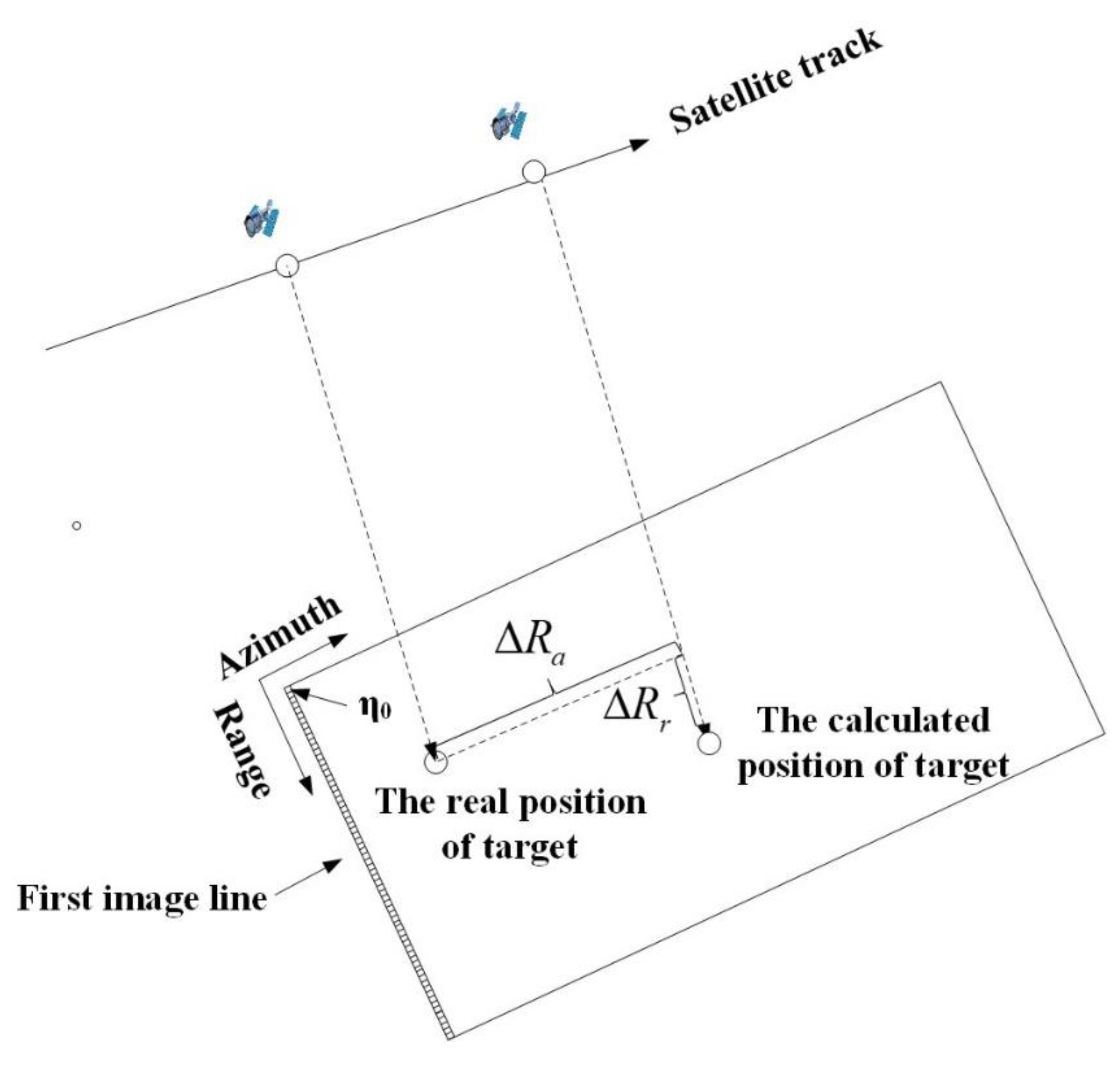
2.3. Geometric Calibration for a Continuously Moving Configuration

Geometric calibration of a SAR system involves the determination of systematic timing offsets in the SAR system, such as systematic azimuth shifts and the slant-range correction, caused by the internal electronic delay of the instrument. These types of timing offsets cause systematic offsets in SAR image pixel locations. The determination of timing offsets is usually accomplished using trihedral corner reflectors (CR). CRs are ideal GCPs for geometric calibration because they involve no additional delay and consequently do not introduce an additional source of error. The geometric calibration model was established by Jiang and Zhang [7]:

$$\{\begin{array}{l}R=R_{near}+r+i\frac{c}{2f_s}\\ {\eta }_p={\eta }_0+t_a+\frac{j}{PRF}\end{array}$$

(8)

where $r$ and $t_a$ represent the slant-range correction and systematic azimuth shifts, respectively.

However, the effect of atmospheric path delay is not considered in the geometric calibration model proposed by Jiang and Zhang. Therefore, it should be compensated for using

$$R=R_{near}+r+{\delta }_{delay}+i\frac{c}{2f_s}$$

(9)

where ${\delta }_{delay}$ is the atmospheric path delay, which is calculated using the atmospheric delay correction model.

Additionally, the geometric calibration model proposed by Jiang and Zhang is based on a “stop-and-go” approximation model. This model assumes that the SAR satellite is stationary during the transmission of the pulse until complete pulse reception and that the satellite then moves to the next position for transmission and reception of the next pulse. However, in reality, the satellite moves a certain distance along its orbit during the time between pulse transmission and echo reception. This is referred to as the bistatic effect or “start-stop” approximation [23], and it is compensated for by using

$${\eta }_p={\eta }_0+t_a+\frac{j}{PRF}-\frac{R_{near}}{c}+\frac{i}{2f_s}.$$

(10)

Therefore, the geometric calibration model for a real continuously moving configuration, including consideration of atmospheric propagation delay, should be written as follows:

$$\{\begin{array}{l}R=R_{near}+r+{\delta }_{delay}+i\frac{c}{2f_s}\\ {\eta }_p={\eta }_0+t_a+\frac{j}{PRF}-\frac{R_{near}}{c}+\frac{i}{2f_s}\end{array}.$$

(11)

The range and azimuth pixel coordinate $\left(i,j\right)$ of the GCP in the image is usually determined by manual identification or using a high-precision point extraction algorithm. The slant-range at the near-range edge $R_{near}$, the azimuth starting time ${\eta }_0$, the pulse repetition frequency $PRF$, and sampling frequency $f_s$ are obtained from the product specifications. $R$ and ${\eta }_p$ are obtained from the ground coordinates, latitude ($lat$), longitude ($lon$), and elevation ($h_t$), of the GCP using the back projection of the RD model. The detailed solution procedure for back projection of the RD model is as follows.

• Obtain $\overrightarrow{R_t}={[x_t,y_t,z_t]}^T$ and $\overrightarrow{V_t}={[v_{t_x},v_{t_y},v_{t_z}]}^T$ for ground target $t$ in the Earth Centered Rotating (ECR) system according to its $lat$, $lon$, and $h_t$.
• Set the initial value of the azimuth imaging time ${\eta }_{p_i}$.
• Using orbit data, the satellite’s position vector $\overrightarrow{R_s}={[x_s,y_s,z_s]}^T$ and velocity vector $\overrightarrow{V_s}={[v_{s_x},v_{s_y},v_{s_z}]}^T$ are calculated for the corresponding azimuth imaging time ${\eta }_{p_i}$ using an interpolation algorithm.
• By substituting $\overrightarrow{R_s}$, $\overrightarrow{V_s}$, $\overrightarrow{ R_t}$, and $\overrightarrow{V_t}$ into the Doppler equation of the RD model (Equation (1)), the Doppler centroid frequency value $f_{De}$ is calculated. Simultaneously, the Doppler centroid frequency value $f_D$ can also be calculated. The change in the azimuth time can then be calculated using the following formula:

  $$dt=\left(f_{De}-f_D\right)/f_D{}^{\prime }$$

  where $f_D{}^{\prime }$ represents the rate of change of the Doppler centroid frequency.
• Update the azimuth imaging time ${\eta }_{p_i}={\eta }_{p_{i-1}}+dt$.
• If $\left|f_{De}-f_D\right|$ < 0.00001, calculate $f_{De}$ and $f_D$, then stop the iteration, export the result ${\eta }_{p_i}$, and go to step 7. Otherwise, return to step 3.
• Calculate the slant-range $R$ using $\overrightarrow{R_s}$ and $\overrightarrow{R_t}$ for the corresponding azimuth imaging time ${\eta }_{p_i}$.

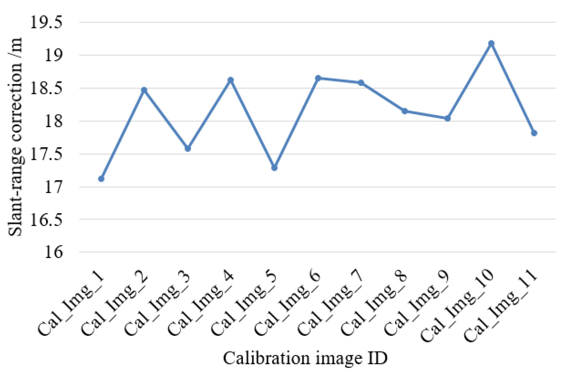
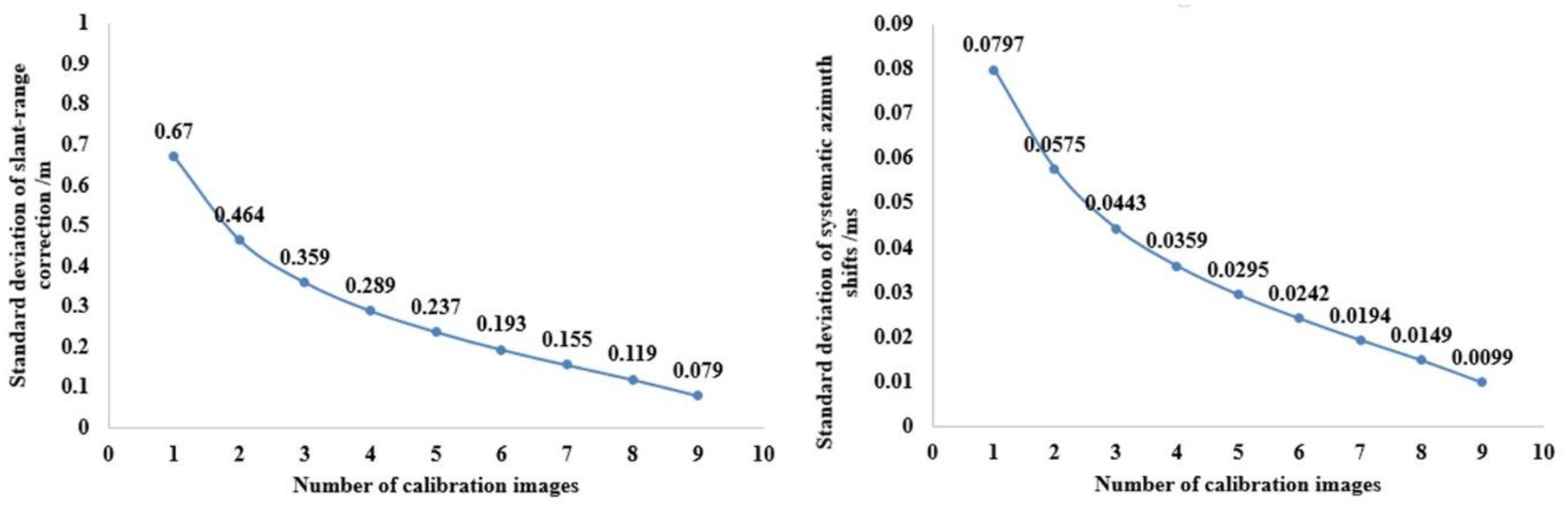
2.4. Multiple-Image Combined Calibration Strategy

According to the geometric calibration model, the main factors affecting the geometric calibration accuracy are orbit accuracy, atmospheric path delay correction accuracy, and GCP coordinate (pixel coordinates and ground coordinates) measurement errors. For a low orbit SAR satellite, precise orbit determination can give an orbit accuracy of the order of decimeters and can sometimes achieve centimeters [17,18,19]. The positioning error caused by errors arising from the atmospheric delay correction model used here is also of the order of the decimeters [1,2].

For a single calibration image, the influence of geometric calibration errors (orbit error, atmospheric path delay correction error, and GCP coordinate measurement errors) on the accuracy of geometric calibration parameters is predominantly manifested as systematic errors. For multiple calibration images in the same area, the effects of geometric calibration errors on the accuracy of geometric calibration parameters show some degree of randomness. Figure 2 shows the slant-range correction obtained using 11 YaoGan-13 images acquired over six months as calibration images.

As can be seen from Figure 2, the geometric calibration errors cause differences in the slant-range corrections obtained using different calibration images, and the difference between the minimum and maximum correction values is more than 2 m. Therefore, to improve the stability of the geometric calibration parameters, multiple images can be combined for calibration and used to achieve a stable solution for the geometric calibration parameters.

The error equations for Equation (11) are as follows:

$$\{\begin{array}{l}{v}_R=\left(R\right)-R+\frac{\partial R}{\partial r}\Delta r+\frac{\partial R}{\partial t_a}\Delta t_a\\ v_{{\eta }_p}=\left({\eta }_p\right)-{\eta }_p+\frac{\partial {\eta }_p}{\partial r}\Delta r+\frac{\partial {\eta }_p}{\partial t_a}\Delta t_a\end{array}$$

(12)

$$V=AX-L,$$

(13)

where

$$V={\left[v_R,v_{{\eta }_p}\right]}^T,$$

$$X={\left[\Delta r,\Delta t_a\right]}^T,$$

$$L={\left[l_R,l_{{\eta }_p}\right]}^T={\left[R-\left(R\right),{\eta }_p-\left({\eta }_p\right)\right]}^T, \mathrm{and}$$

$$A={\left[\begin{array}{c}{a}_{11},a_{12}\\ a_{21},a_{22}\end{array}\right]}^T.$$

The values of the partial derivatives in Equation (12) are as follows: $a_{11}=1$; $a_{12}=0$; $a_{21}=0$; and $a_{22}=1$.

In Equation (12), $R$ and ${\eta }_p$ are observed values calculated from the ground coordinates $\left(lat,lon,h_t\right)$ of the GCP through the back projection of the RD model. $\left(R\right)$ and $\left({\eta }_p\right)$ are obtained by substituting the approximate value of the slant-range correction $\Delta r$ and systematic azimuth shifts $\Delta t_a$ into Equation (12). The initial values of the geometric calibration parameters are as follows: $\Delta r^0=0,\Delta t_a{}^0=0$. An iterative procedure was adopted to calculate ${\left[\Delta r,\Delta t_a\right]}^T$:

$$\{\begin{array}{l}\Delta r=\Delta r^0+\Delta r^1+\Delta r^2+\cdots \\ \Delta t_a=\Delta t_a{}^0+\Delta t_a{}^1+\Delta t_a{}^2+\cdots \end{array}.$$

(14)

When a multiple-image combined calibration strategy is adopted, k calibration images are obtained and n control points are selected for each calibration scene. The $2\ast k\ast n$ error equation can be established according to Equation (12). Using several GCPs, $\Delta r$ and $\Delta t_a$ can be calculated based on the least squares method.

3. Experimental Results

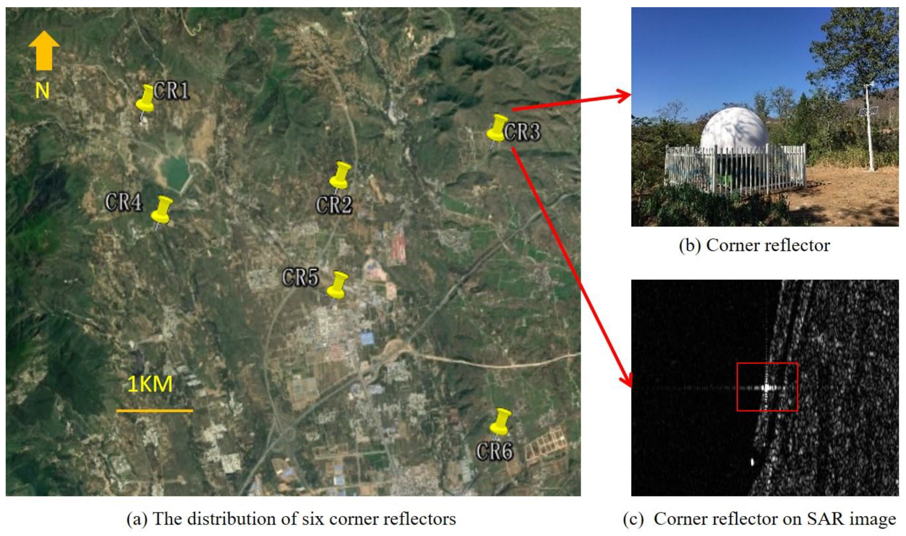
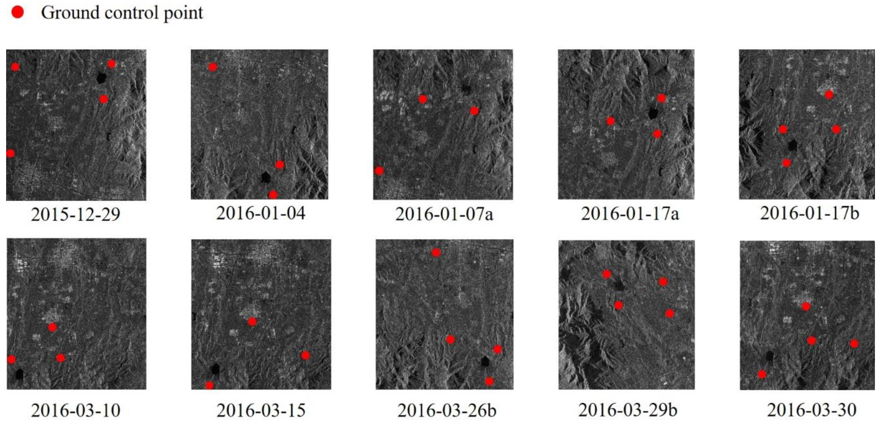
3.1. Multiple-Image Combined Calibration Strategy

Two datasets (A and B) were adopted to validate the multiple-image combined calibration strategy. Dataset A consists of ten YaoGan-13 images taken in stripmap mode over the Songshan calibration field. The slant-range correction and systematic azimuth shifts for the YaoGan-13 sensor were calculated using dataset A. Dataset B was used to validate the absolute positioning accuracy of YaoGan-13 that was determined using the calculated slant-range corrections and systematic azimuth shifts. To gain full and reliable experimental data to verify the geometric calibration result, YaoGan-13 images obtained using stripmap mode over five test fields (Figure 3) were included in dataset B. All the images in datasets A and B were corrected for atmospheric path delay.

Table 3. Experimental image specifications for dataset A.

Satellite	Imaging Mode	Test Field	Imaging Date	Incidence Angle (°)	Orbit	Look Side
YaoGan-13	Stripmap-1 mode (resolution: 1.5 m)	Songshan	29 December 2015	46.1	Desc	R
			04 January 2016	46.9	Asc	L
			07a January 2016	54.6	Desc	R
			17a January 2016	50.9	Desc	R
			17b January 2016	48.9	Asc	R
			10 March 2016	45.5	Asc	R
			15 March 2016	48.0	Asc	R
			26b March 2016	50.4	Asc	L
			29b March 2016	38.0	Asc	R
			30 March 2016	53.8	Asc	R

Desc = Descending; Asc = Ascending; L = Left; R = Right.

and

Table 4. Experimental image specifications for dataset B.

Satellite	Imaging Mode	Test Field	Imaging Date	Incidence Angle (°)	Orbit	Look Side
YaoGan-13	Stripmap-1 mode (resolution: 1.5 m)	Songshan	02 April 2016	45.7	Desc	L
		Taiyuan	01 June 2016	48.8	Desc	R
		Anping	09 June 2016	49.9	Desc	L
		Tianjin	10 June 2016	45.5	Desc	R
		Xianning	12 June 2016	46.5	Asc	L

list the experimental image specifications.

Six CRs are installed at the Songshan test field, which can be used as GCPs for geometric calibration, as shown in Figure 4. We measured their positions with a GPS and obtained a 3-D position accuracy of within 0.3 m horizontally and 0.1 m vertically. For a CR, the brightest position on the image represents the pixel coordinate of the CR vertex. Interpolation was performed to determine the peak position of the CR’s impulse response function.

Different control data (Figure 5) were used to obtain ICPs for the five geolocation test fields to validate the absolute positioning accuracy after geometric calibration. ICP information for the five test fields is as follows.

• Songshan test field: six CRs were used as ICPs.
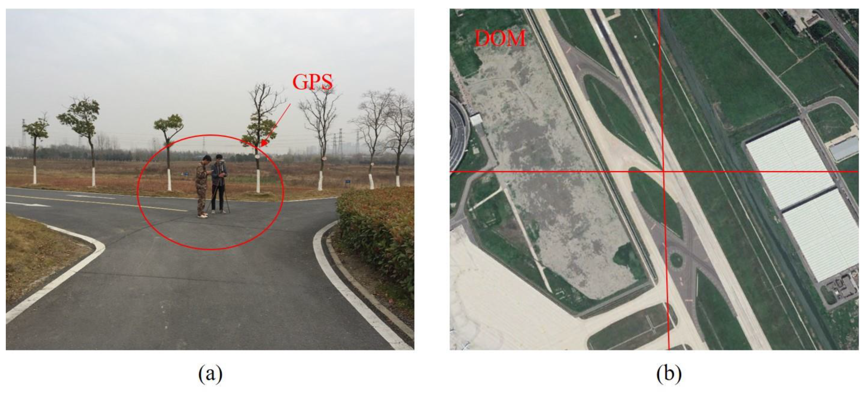
• Taiyuan and Tianjin test fields: the 1:5000-scale digital orthophoto map (DOM) and Digital Elevation Model (DEM) of the Taiyuan region and the 1:2000-scale DOM and DEM of the Tianjin region were used as control data to obtain ICPs. Their planimetric accuracies and height accuracies are both <1m. Natural targets, such as road intersections, water bodies, or field boundaries, were used throughout to serve as ICPs. The latitudes and longitudes of checkpoints were obtained from the DOM, and their elevations were obtained from the DEM.
• Anping and Xianning test fields: the Xianning and Anping test fields contain a large number of GPS control points with plane and elevation accuracies of 0.3 m and 0.1 m, respectively.

The number of GCPs used for image calibration is shown in Figure 6. As mentioned above, dataset A contains ten calibration images. A large number of image combinations can be obtained by selecting different numbers of calibration images. The number of permutations and combinations for different numbers of calibration images is shown in

Table 5. Combinations for different numbers of images.

Number of Calibration Images	1	2	3	4	5	6	7	8	9
Number of image permutations	10	45	120	210	252	210	120	45	10

.

The slant-range correction and systematic azimuth shifts of the YaoGan-13 sensor were calculated using different numbers of calibration images.

Table 6. Standard deviations of the slant-range correction and systematic azimuth shift results.

Number of Calibration Images	1	2	3	4	5	6	7	8	9
Standard deviation of slant-range correction $\sigma \left(r\right)$ (m)	0.670	0.464	0.359	0.289	0.237	0.193	0.155	0.119	0.079
Standard deviation of systematic azimuth shifts $\sigma \left(t_a\right)$ (ms)	0.079	0.057	0.044	0.035	0.029	0.024	0.019	0.014	0.009

shows the standard deviation statistics for the calculation results. When the number of selected calibration images is 1, we take this as an example to illustrate Table 6. As shown in Table 3, there are ten calibration images, we can get ten slant-range corrections ($r_1,r_2,\cdots ,r_9,r_{10}$) and ten systematic azimuth shifts ($t_{a_1},t_{a_2},\cdots ,t_{a_9},t_{a_{10}}$). The standard deviation of slant-range correction $\sigma \left(r\right)$ is given by

$$\{\begin{array}{l}\mu \left(r\right)=\frac{r_1+r_2+\cdots +r_{10}}{10}\\ \sigma \left(r\right)=\sqrt{\frac{1}{10}{\displaystyle {\displaystyle \sum }_{i=1}^{10}}{\left(r_i-\mu \left(r\right)\right)}^2}\end{array}$$

(15)

The standard deviation of systematic azimuth shifts $\sigma \left(t_a\right)$ is given by

$$\{\begin{array}{l}\mu \left(t_a\right)=\frac{t_{a_1}+t_{a_2}+\cdots +t_{a_{10}}}{10}\\ \sigma \left(t_a\right)=\sqrt{\frac{1}{10}{\displaystyle {\displaystyle \sum }_{i=1}^{10}}{\left(t_a{}_i-\mu \left(t_a\right)\right)}^2}\end{array}$$

(16)

As can be seen from Figure 7, the standard deviations of the slant-range corrections and systematic azimuth shifts decreases as the number of calibration images involved in the geometric calibration increases (i.e., the calibration result is more stable).

To further illustrate the effectiveness of the multiple-image combined calibration strategy using dataset A’s calibration images, the number of images used in the calibration was sequentially increased. Images over five test fields were then adopted to evaluate the absolute positioning accuracy obtained using the ten-image calculated slant-range corrections and systematic azimuth shifts. We calculated the root-mean-square error (RMSE) of the absolute position (north, east, and plane) for images over five test fields. “Plane” indicates the size of the RMSE in the plane of the object’s space, which is numerically equal to the square root of the sum of the squares of the “east” and “north” errors. As can be seen from Figure 8, the plane absolute positioning accuracy improved from 2.51 m to 1.71 m as the number of calibration images involved in the geometric calibration increased. The accuracy of the geometric calibration is predominantly affected by the orbit accuracy, the accuracy of the atmospheric delay correction model, and the accuracy of control points. Therefore, the addition of calibration images will lead to additional errors, resulting in a slight fluctuation in the whole result. However, the multiple-image combined calibration strategy can effectively reduce the influence of random errors in the geometric calibration process, improving the absolute positioning accuracy of images.

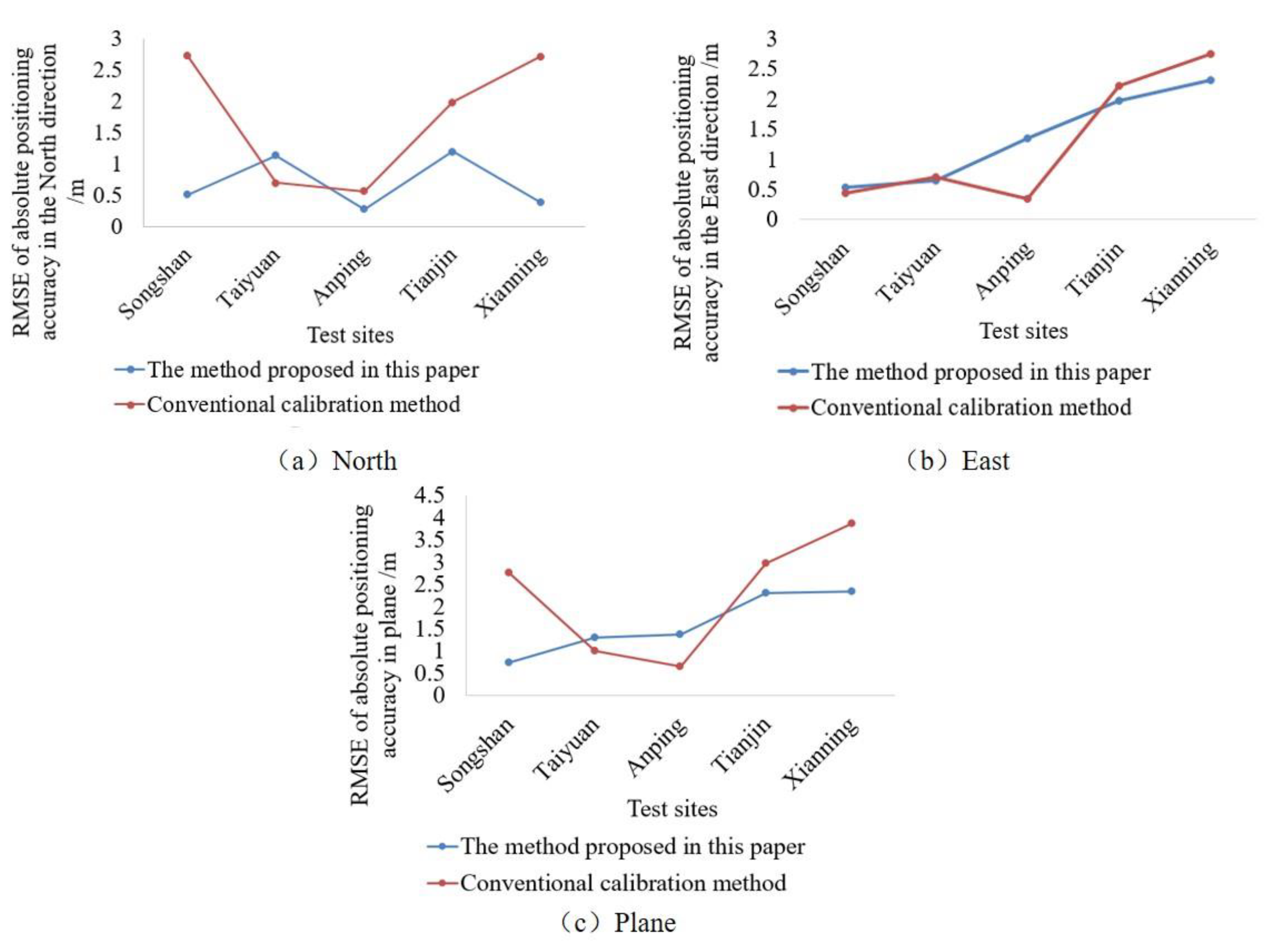
3.2. Comparison of our Geometric Calibration Method and the Conventional Calibration Method

The geometric calibration method proposed by Jiang and Zhang [7] does not consider the error introduced by the “stop and go” approximation model or the influence of atmospheric path delay [8]. This conventional calibration method is, therefore, not applicable to the geometric calibration of existing high-resolution SAR images. In contrast, the geometric calibration method proposed here accounts for the “stop and go” approximation and atmospheric path delay. Datasets A and B (Section 3.1) were used as experimental data to compare the geometric calibration method proposed here with the traditional calibration method. The slant-range correction and systematic azimuth shifts of the YaoGan-13 sensor were calculated using the ten calibration images in dataset A. Images from dataset B were then adopted to evaluate the absolute positioning accuracy obtained using the calculated slant-range corrections and systematic azimuth shifts.

Table 7. Geometric calibration parameters solved using the two geometric calibration methods.

Method	Direction	Item	Value
Conventional calibration method	Range	Slant-range correction	+13.030 m
	Azimuth	Systematic azimuth shift	−0.00373 s
The method proposed in this paper	Range	Slant-range correction	+17.371 m
	Azimuth	Systematic azimuth shift	−0.000111 s

lists the geometric calibration parameters for YaoGan-13 solved using the two geometric calibration methods and shows that both the slant-range correction and systematic azimuth shift are different for the two different methods. The result is consistent with the physical imaging process. As shown in Figure 9, the error $\Delta R_a$ introduced by the “stop and go” approximation model affects the azimuth direction of the image and the error $\Delta R_r$ introduced by the atmospheric path delay affects the range direction of the image.

Statistical results comparing the absolute positioning accuracy of YaoGan-13 calculated using the conventional calibration method with the accuracy calculated using the method proposed here are shown in Figure 10. The results show that, in the majority of cases, the accuracy achieved by the geometric calibration method proposed in this paper was better than that achieved by the conventional calibration method.

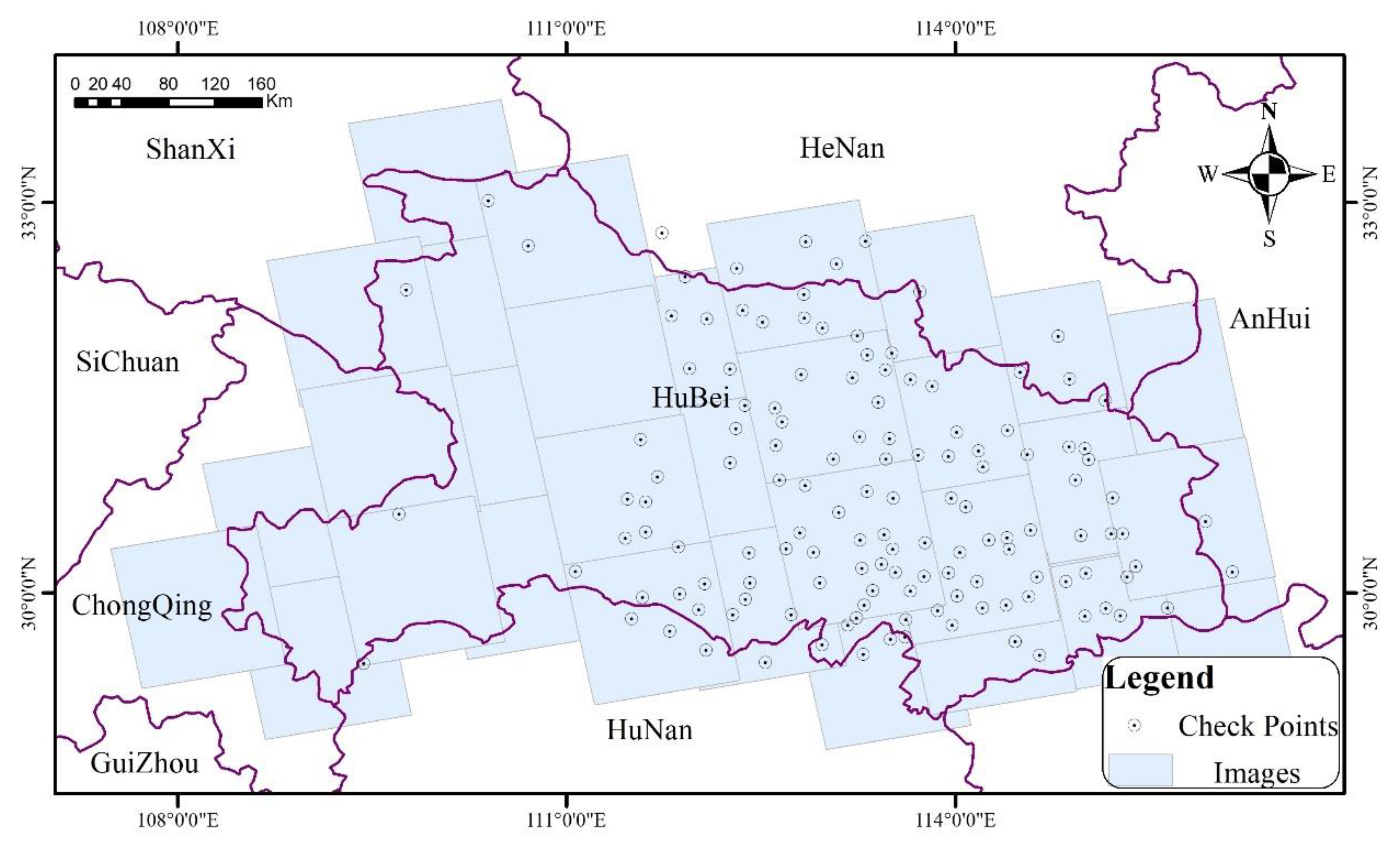
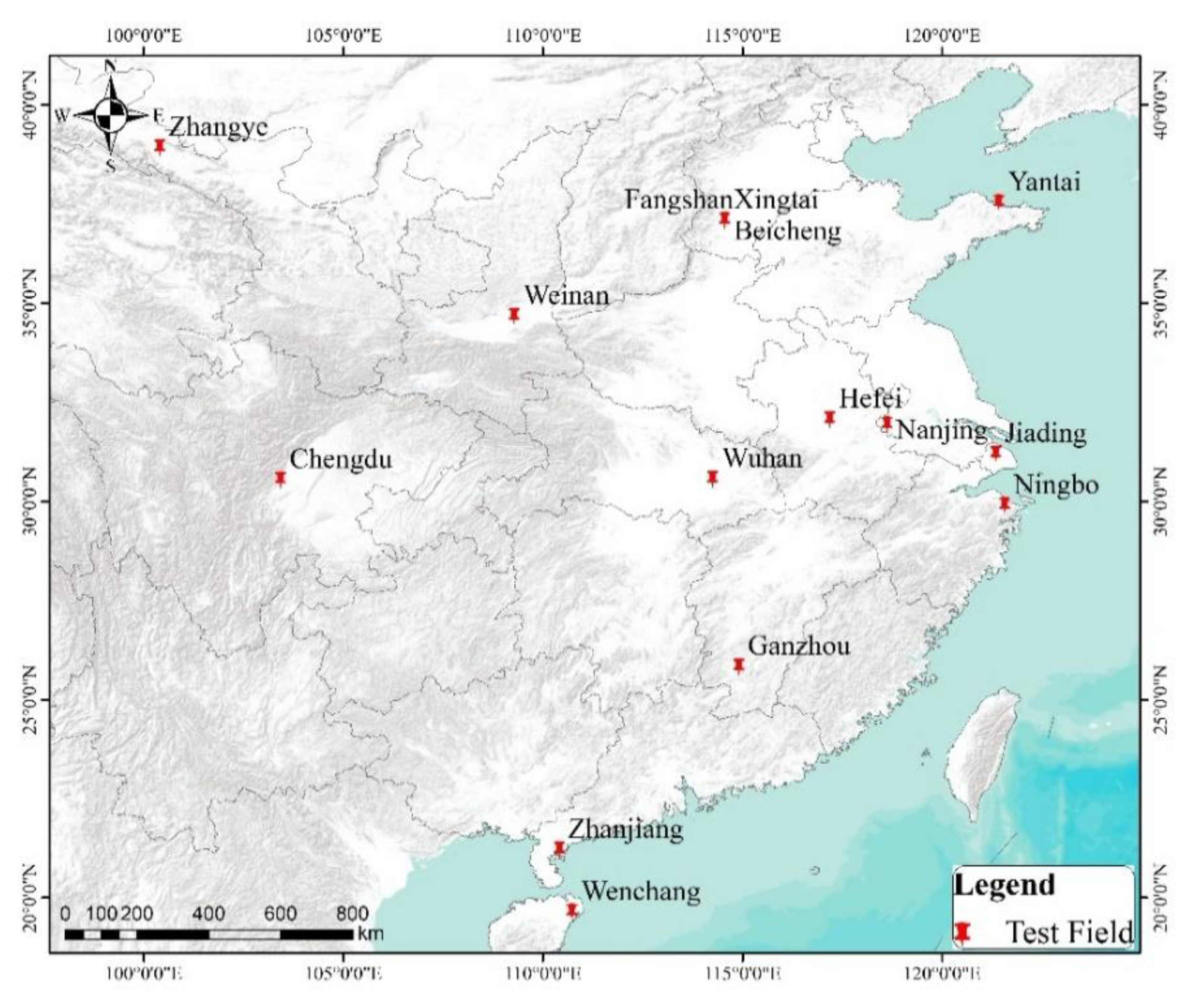
3.3. Assessment of the Absolute Positioning Accuracy for YaoGan-13 and GaoFen-3

The discussion in Section 3.1 concluded that the multiple-image combined calibration strategy improves the stability of the calibration result. Section 3.2. proves the validity of the geometric calibration method proposed in this paper. The multiple-image combined calibration strategy and geometric calibration method proposed in this paper were applied to the geometric calibration of YaoGan-13 and GaoFen-3, and we assessed the absolute positioning accuracies of YaoGan-13 and GaoFen-3 on a large scale. The assessments carried out to determine the validity of our new method are listed as follows.

Absolute positioning accuracy of a single image: We calculated the RMSE of the absolute positioning accuracy (north, east, and plane) for YaoGan13 and GaoFen-3 before and after compensating for geometric calibration parameters. The resulting statistical information for five test fields is listed in

Table 8. Comparison of absolute positioning accuracy of YaoGan-13 and GaoFen-3 before and after compensating for geometric calibration parameters (for a single image).

Satellite	Imaging Mode (Resolution)	Test Field	Imaging Date	Calibration	Absolute Positioning Accuracy (m)
					North	East	Plane
YaoGan-13	Stripmap-1 (1.5 m)	Songshan	02 April 2016	Before	4.79	21.93	22.45
				After	0.42	0.50	0.65
		Taiyuan	01 June 2016	Before	4.23	20.43	20.87
				After	0.91	0.63	1.11
		Anping	09 June 2016	Before	6.46	20.99	21.96
				After	0.46	1.25	1.33
		Tianjin	10 June 2016	Before	4.95	23.78	24.29
				After	1.06	1.98	2.24
		Xianning	12 June 2016	Before	6.28	23.25	24.08
				After	0.32	2.33	2.35
	Stripmap-2 (1.5 m)	Songshan	29b March 2016	Before	4.44	25.11	25.50
				After	0.41	0.94	1.02
		Taiyuan	28 May 2016	Before	6.98	30.06	30.87
				After	1.39	0.46	1.46
		Tianjin	29 May 2016	Before	8.69	30.45	31.66
				After	1.09	0.86	1.39
	Slidingspot-1 (1 m)	Xianning	21 May 2016	Before	4.68	37.12	37.41
				After	1.85	1.78	2.57
		Tianjin	22 May 2016	Before	5.26	31.43	31.87
				After	1.18	1.66	2.04
	Slidingspot-2 (1 m)	Songshan	05 January 2016	Before	10.82	42.50	43.86
				After	0.23	0.68	0.72
		Taiyuan	21 May 2016	Before	7.04	35.14	35.84
				After	0.85	1.34	1.59
GaoFen-3	Stripmap-1 (5 m)	Taiyuan	30 December 2016	Before	3.25	30.17	30.34
				After	1.73	3.20	3.64
		Taiyuan	11 January 2017	Before	3.66	27.81	28.05
				After	2.53	2.03	3.25
	Stripmap-2 (5 m)	Tianjin	17 February 2017	Before	7.25	24.92	25.96
				After	1.20	4.12	4.29
		Tianjin	18 March 2017	Before	7.09	27.55	28.45
				After	1.70	3.86	4.22

.

As can been see from Table 8, without geometric calibration, the absolute positioning accuracies for YaoGan-13 and GaoFen-3 are poor. In the worst case, the “plane” absolute positioning accuracies for YaoGan-13 and GaoFen-3 are 43.86 m and 30.34 m, respectively. After geometric calibration, the results indicate that high-accuracy absolute positioning can now be achieved with a “plane” accuracy of 2.57 m or better for YaoGan-13 and of 4.29 m or better for GaoFen-3, without regard to the elevation error. The absolute positioning accuracy (“plane”) is mainly limited by the “east” geolocation accuracy. Based on the spatial geometry model for spaceborne SAR, we found that the “east” geolocation accuracy is predominantly affected by the slant-range accuracy. Therefore, the slant-range accuracy is the most important factor restricting the absolute positioning accuracy of YaoGan-13 and GaoFen-3.

Absolute positioning accuracy for a large-area mosaic image: In some cases, a single image cannot meet the accuracy requirements for a wide range of national census geography applications. Therefore, a large-area mosaic image was required. The absolute positioning accuracy of the large-area mosaic image is also important, and we selected Hubei province as the test area to evaluate its accuracy. For Hubei province, nine-track data, including 31 GaoFen-3 images after geometric calibration, were available (Figure 11). Further details regarding the test area are listed in

Table 9. Parameters of the test area.

Test Area	Satellite	Imaging Mode	Ground Resolution (m)	Number of Checkpoints
Hubei province	GaoFen-3	Stripmap-3	10 m	135

.

The large-area mosaic image was created using the method described in Reference [25]. We calculated the RMSE of the absolute positioning accuracy (north, east, and plane) of the GaoFen-3 large-area mosaic image. The resulting statistical information is listed in

Table 10. The absolute positioning accuracy of GaoFen-3 for the large-area mosaic image.

Test Field	GCPs	ICPs	Calibration	Maximum Residual (m)			RMSE (m)
				East	North	Plane	East	North	Plane
Hubei province	0	135	Before	54.80	13.74	55.01	38.70	4.54	38.97
			After	14.90	−17.98	19.10	4.60	7.70	8.97

. After geometric calibration, the statistical plane absolute positioning accuracy was improved from 38.97 m (RMSE) to 8.97 m (RMSE). Considering the image resolution of 10 m, the experimental result shows that sub-pixel localization accuracy was achieved for the GaoFen-3 Stripmap-3 mode.

Three-dimensional absolute positioning accuracy: Based on the high absolute positioning accuracy of the YaoGan-13 image after geometric calibration and the use of stereo pairs, the corresponding 3-D ground coordinates can be calculated using a least squares spatial point intersection. The 3-D absolute geolocation accuracy of YaoGan-13 can then be assessed. To validate the 3-D absolute positioning accuracy of the YaoGan-13 image after calibration, we selected 15 test fields in China (Figure 12), and a stereo pair was selected for each test field. The RMSE of the 3-D point residuals achieved for “north,” “east,” “plane,” and “height” are summarized in

Table 11. Results of the 3-D accuracy assessment.

Satellite	Imaging Mode (Resolution)	Test Field	ICPs	Intersection Angle(°)	Absolute Positioning Accuracy (m)
					North	East	Plane	Height
YaoGan-13	Sliding spot (1 m)	Zhangye	11	63	0.90	0.83	1.22	2.56
		Chengdu	19	88	1.32	0.78	1.53	0.82
		Weinan	10	80	0.96	2.01	2.22	1.85
		Xingtai	19	64	1.18	0.92	1.49	0.92
		Wuhan	11	77	0.92	2.94	3.08	1.04
		Ganzhou	11	71	2.88	4.83	5.62	3.14
		Zhanjiang	14	76	1.03	0.44	1.12	1.62
		Wenchang	18	80	0.64	2.68	2.75	1.07
		Beichen	20	75	1.36	2.07	2.47	2.00
		Fangshan	16	48	1.57	0.61	1.68	0.55
		Hefei	14	65	1.80	3.70	4.11	1.11
		Nanjing	15	79	1.49	2.15	2.61	1.64
		Yantai	19	68	1.46	6.83	6.98	2.06
		Jiading	22	77	1.47	2.16	2.61	2.32
		Ningbo	21	98	2.08	0.82	2.23	5.45
RMSE					-	-	3.21	2.22

.

These values represent the feasible 3-D mapping accuracy for YaoGan-13 stereo pairs. We calculated the RMSEs of all ICP residuals over the fifteen test fields. The accuracies for “plane” and “height” were 3.21 m and 2.22 m, respectively, satisfying the requirements for high-precision three-dimensional control points. A wide range of test results show that the improved absolute positioning accuracy method achieved good results for YaoGan-13.

4. Discussion

4.1. Geometric Calibration Parameters

Without considering external factors such as elevation error and atmospheric propagation delay error, the absolute positioning accuracy of satellite image is mainly caused by the hardware error of the SAR system. As can been see from

Table 12. Geolocation error caused by the internal electronic delay of the instrument and systematic azimuth shift.

Satellite	Imaging Mode	Slant-Range Correction (m)	Systematic Azimuth Shift (s)	Geolocation Error (m)
				Range	Azimuth
YaoGan-13	Stripmap-1 (1.5 m)	+17.371	−0.000111	17.371	0.843
	Stripmap-2 (1.5 m)	+17.856	−0.000101	17.856	−0.767
	Slidingspot-1 (1 m)	+20.543	+0.000067	20.543	0.509
	Slidingspot-2 (1 m)	+19.834	+0.000064	19.834	0.486
GaoFen-3	Stripmap-1 (5 m)	−18.838	+0.000494	18.838	3.754
	Stripmap-2 (5 m)	−20.886	+0.000212	20.886	1.611

, given a spacecraft velocity of 7600 $m\cdot s^{-1}$, the range geolocation error caused by the internal electronic delay of the instrument is larger than the azimuth geolocation error caused by systematic azimuth shift. It can be drawn that the internal electronic delay of the instrument has become the most important factor affecting the correct localization of YaoGan-13 and GaoFen-3 images. With the development of SAR hardware, the synchronization accuracy of the SAR local clock relative to the time benchmark of the whole satellite improved a lot.

4.2. Accuracy Loss Analysis

In the process of improvement and assessment of absolute positioning accuracy, there exist links of precision loss: orbit accuracy, atmospheric path delay, and acquisition of GCPs and ICPs. As a result of using precise orbit determination, the orbit accuracies of YaoGan-13 and GaoFen-3 are better than 0.3 m and 0.05 m, respectively. The accuracy of the atmospheric propagation delay correction used in this study is better than 0.2 m. Generally speaking, the accuracies of the GCP and ICP are about 1 pixel. With the reduction of the image resolution, the absolute positioning accuracy of the image assessed by ICPs is also decreasing. Therefore, as shown in Table 8 and Table 10, after calibration, GaoFen-3 demonstrates poorer absolute positioning performance than that of YaoGan-13. Meanwhile, the absolute positioning accuracy of GaoFen-3 Stripmap-3 is poorer than that of GaoFen-3 Stripmap-1 and Stripmap-2.

5. Conclusions

The launch of YaoGan-13 and GaoFen-3 provided China with the ability to acquire global high-resolution SAR images. The absolute positioning accuracy is very important for the application of these satellite to activities such as resource monitoring and disaster monitoring. Absolute measurements of volcanoes or earthquakes are possible without the use of ground equipment and without the use of SAR interferometry [26]. In this study, based on the characteristics of systematic errors, we established a geometric calibration for a continuously moving configuration and proposed a multiple-image combined calibration strategy. We also assessed the 2-D/3-D geolocation accuracy of YaoGan-13 and GaoFen-3 images, based on the utilization of natural and man-made control points. Our results suggest the following conclusions.

• The internal electronic delay of the instrument is the main error source for the absolute positioning of spaceborne SAR. Use of the methods proposed here can improve absolute positioning accuracy significantly.
• For high resolution spaceborne SAR, the effects of the atmospheric path delay and the “start-stop” approximation on the geometric calibration accuracy should be considered.
• Without using GCPs, a high geolocation accuracy can be ensured for YaoGan-13 and GaoFen-3. In terms of absolute positioning accuracy, domestic SAR satellites are comparable to typical international SAR satellites, such as TerraSAR-X and Sentinel-1A/1B.

In summary, we have shown that the method presented in this paper can enable YaoGan-13 and GaoFen-3 to deliver satisfactory absolute positioning accuracy.

References

1. Deng, M.; Zhang, G.; Zhao, R.; Zhang, Q.; Li, D.; Li, J. Assessment of the geolocation accuracy of YG-13A high-resolution SAR data. Remote Sens. Lett. 2018, 9, 101–110. [Google Scholar] [CrossRef]
2. Deng, M.; Zhang, G.; Zhao, R.; Li, S.; Li, J. Improvement of Gaofen-3 Absolute Positioning Accuracy Based on Cross-Calibration. Sensors 2017, 17, 2903. [Google Scholar] [CrossRef] [PubMed]
3. Schubert, A.; Miranda, N.; Geudtner, D.; Small, D. Sentinel-1A/B Combined Product Geolocation Accuracy. Remote Sens. 2017, 9, 607. [Google Scholar] [CrossRef]
4. Raggam, H.; Gutjahr, K.; Perko, R.; Schardt, M. Assessment of the Stereo-Radargrammetric Mapping Potential of TerraSAR-X Multibeam Spotlight Data. IEEE Trans. Geosci. Remote Sens. 2010, 48, 971–977. [Google Scholar] [CrossRef]
5. Liu, X.; Ma, H.; Sun, W. Study on the Geolocation Algorithm of Space-Borne SAR Image. In Advances in Machine Vision, Image Processing, and Pattern Analysis; Zheng, N., Jiang, X., Lan, X., Eds.; Lecture Notes in Computer Science; Springer: Berlin/Heidelberg, Germany, 2006; Volume 4153. [Google Scholar]
6. Zhao, R.; Jiang, Y.; Zhang, G.; Deng, M.; Yang, F. Geometric Accuracy Evaluation of YG-18 Satellite Imagery Based on RFM. Photogramm. Rec. 2017, 32, 33–47. [Google Scholar] [CrossRef] [Green Version]
7. Hua, J.; Zhang, G. Research on the methods of inner calibration of spaceborne SAR. In Proceedings of the 2011 IEEE International Geoscience and Remote Sensing Symposium (IGARSS), Vancouver, BC, Canada, 24–29 July 2011; pp. 914–916. [Google Scholar]
8. Mohr, J.J.; Madsen, S.N. Geometric calibration of ERS satellite SAR images. IEEE Trans. Geosci. Remote Sens. 2001, 39, 842–850. [Google Scholar] [CrossRef]
9. Small, D.; Rosich, B.; Meier, E.; Nüesch, D. Geometric calibration and validation of ASAR imagery. In Proceedings of the CEOS SAR Workshop 2004, Ulm, Germany, 27–28 May 2004. [Google Scholar]
10. Cote, S.; Srivastava, S.; Muir, S.; Hawkins, R.; Lukowski, T. RADARSAT-1 AND-2 government calibration activities. In Proceedings of the 2009 IEEE International Geoscience and Remote Sensing Symposium (IGARSS), Cape Town, South Africa, 12–17 July 2009; p. II-890. [Google Scholar]
11. Shimada, M.; Isoguchi, O.; Tadono, T.; Isono, K. PALSAR Radiometric and Geometric Calibration. IEEE Trans. Geosci. Remote Sens. 2009, 47, 3915–3932. [Google Scholar] [CrossRef]
12. Nitti, D.O.; Nutricato, R.; Lorusso, R.; Lombardi, N.; Bovenga, F.; Bruno, M.F.; Chiaradia, M.T.; Milillo, G. On the geolocation accuracy of COSMO-SkyMed products. In Proceedings of the SAR Image Analysis, Modeling, and Techniques XV; SPIE: Bellingham, WA, USA, 2015; Volume 9642, p. 96420D. [Google Scholar]
13. Schwerdt, M.; Brautigam, B.; Bachmann, M.; Doring, B.; Schrank, D.; Gonzalez, J.H. Final TerraSAR-X Calibration Results Based on Novel Efficient Methods. IEEE Trans. Geosci. Remote Sens. 2010, 48, 677–689. [Google Scholar] [CrossRef]
14. Schwerdt, M.; Schrank, D.; Bachmann, M.; Gonzalez, J.H.; Döring, B.J.; Tous-Ramon, N.; Antony, J.W. Calibration of the TerraSAR-X and the TanDEM-X satellite for the TerraSAR-X mission. In Proceedings of the 9th European Conference on Synthetic Aperture Radar; VDE: Frankfurt, Germany, 2012; pp. 56–59. [Google Scholar]
15. Schwerdt, M.; Schmidt, K.; Ramon, N.T.; Alfonzo, G.C.; Döring, B.J.; Zink, M.; Prats-Iraola, P. Independent verification of the Sentinel-1A system calibration. Geosci. Remote Sens. Symp. 2014, 9, 994–1007. [Google Scholar]
16. Schwerdt, M.; Schmidt, K.; Tous Ramon, N.; Klenk, P.; Yague-Martinez, N.; Prats-Iraola, P.; Zink, M.; Geudtner, D. Independent System Calibration of Sentinel-1B. Remote Sens. 2017, 9, 511. [Google Scholar] [CrossRef]
17. Guo, X.; Zhang, Q.; Zhao, Q.; Guo, J. Precise orbit determination for LEO satellites using single-frequency GPS observations. Chin. Space Sci. Technol. 2013, 33, 41–46. [Google Scholar]
18. Eineder, M.; Minet, C.; Steigenberger, P.; Cong, X.; Fritz, T. Imaging Geodesy—Toward Centimeter-Level Ranging Accuracy with TerraSAR-X. IEEE Trans. Geosci. Remote Sens. 2011, 49, 661–671. [Google Scholar] [CrossRef]
19. Ding, C.; Liu, J.; Lei, B.; Qiu, X. Preliminary exploration of systematic geolocation accuracy of GF-3 SAR satellite system. J. Radars 2017, 6, 11–16. [Google Scholar] [CrossRef]
20. Schubert, A.; Jehle, M.; Small, D.; Meier, E. Influence of Atmospheric Path Delay on the Absolute Geolocation Accuracy of TerraSAR-X High-Resolution Products. IEEE Trans. Geosci. Remote Sens. 2010, 48, 751–758. [Google Scholar] [CrossRef]
21. Jehle, M.; Perler, D.; Small, D.; Schubert, A.; Meier, E. Estimation of Atmospheric Path Delays in TerraSAR-X Data using Models vs. Measurements. Sensors 2008, 8, 8479–8491. [Google Scholar] [CrossRef] [PubMed]
22. Li, S.; Zhang, G.; Tang, X.; Huang, W. A method for detecting the atmospheric refraction effect using satellite remote sensing. Remote Sens. Lett. 2016, 7, 985–993. [Google Scholar] [CrossRef]
23. Schubert, A.; Small, D.; Miranda, N.; Geudtner, D.; Meier, E. Sentinel-1A Product Geolocation Accuracy: Commissioning Phase Results. Remote Sens. 2015, 7, 9431–9449. [Google Scholar] [CrossRef] [Green Version]
24. Deng, M.; Zhang, G.; Zhao, R.; Li, S.; Li, J. Application of the atmospheric delay correction model in YG-13A range calibration. J. Remote Sens. 2018, 22, 373–380. [Google Scholar]
25. Wang, T.; Zhang, G.; Li, D.; Zhao, R.; Deng, M.; Zhu, T.; Yu, L. Planar block adjustment and orthorectification of Chinese spaceborne SAR YG-5 imagery based on RPC. Int. J. Remote Sens. 2018, 39, 640–654. [Google Scholar] [CrossRef]
26. Merryman Boncori, J.P.; Papoutsis, I.; Pezzo, G.; Tolomei, C.; Atzori, S.; Ganas, A.; Karastathis, V.; Salvi, S.; Kontoes, C.; Antonioli, A. The February 2014 Cephalonia Earthquake (Greece): 3D Deformation Field and Source Modeling from Multiple SAR Techniques. Seismol. Res. Lett. 2015, 86, 124–137. [Google Scholar] [CrossRef]
Figure 1. Influence of atmospheric path delay on slant-range.
Remotesensing 11 01465 g001
Figure 2. YaoGan-13 slant-range corrections calculated using 11 calibration images.
Remotesensing 11 01465 g002
Figure 3. Distribution of the five test fields in China.
Remotesensing 11 01465 g003
Figure 4. Songshan test field [24]. (a) The distribution of six corner reflectors; (b) Corner reflector; (c) Corner reflector on SAR image.
Remotesensing 11 01465 g004
Figure 5. (a) GPS control point used for the Xianning and Anping test fields; (b) control point manually extracted from digital orthophoto map (DOM)/Digital Elevation Model (DEM) imagery at the Tianjin and Taiyuan test fields.
Remotesensing 11 01465 g005
Figure 6. The number of ground control points (GCPs) used for image calibration in Table 3.
Remotesensing 11 01465 g006
Figure 7. Trends in standard deviations for the slant-range corrections and systematic azimuth shifts with the number of calibration images used for calculation.
Remotesensing 11 01465 g007
Figure 8. Variations in the root-mean-square error (RMSE) of the absolute positioning accuracy (north, east, and plane) computed on independent checkpoints (ICPs) with the number of calibration images.
Remotesensing 11 01465 g008
Figure 9. Positioning error introduced by the “stop and go” approximation model and the atmospheric path delay.
Remotesensing 11 01465 g009
Figure 10. Comparison of the conventional geometric calibration method with the method proposed in this paper. (a) North; (b) East; (c) Plane.
Remotesensing 11 01465 g010
Figure 11. Gaofen-3 large-area mosaic image of Hubei province.
Remotesensing 11 01465 g011
Figure 12. Distribution of the fifteen periodic test fields for Yaogan-13 in China.
Remotesensing 11 01465 g012