Developing an Aircraft-Based Angular Distribution Model of Solar Reflection from Wildfire Smoke to Aid Satellite-Based Radiative Flux Estimation

Abstract

This study examines the angular distribution of scattered solar radiation associated with wildfire smoke aerosols observed over boreal forests in Canada during the ARCTAS (Arctic Research of the Composition of the Troposphere from Aircraft and Satellites) campaign. First, it estimates smoke radiative parameters (550 nm optical depth of 3.9 and single scattering albedo of 0.90) using quasi-simultaneous multiangular and multispectral airborne measurements by the Cloud Absorption Radiometer (CAR). Next, the paper estimates the broadband top-of-atmosphere radiances that a satellite instrument such as the Clouds and the Earth’s Radiant Energy System (CERES) could have observed, given the narrowband CAR measurements made from an aircraft circling about a kilometer above the smoke layer. This estimation includes both an atmospheric correction that accounts for the atmosphere above the aircraft and a narrowband-to-broadband conversion. The angular distribution of estimated radiances is found to be substantially different than the angular model used in the operational data processing of CERES observations over the same area. This is because the CERES model is a monthly average model that was constructed using observations taken under smoke-free conditions. Finally, a sensitivity analysis shows that the estimated angular distribution remains accurate for a fairly wide range of smoke and underlying surface parameters. Overall, results from this work suggest that airborne CAR measurements can bring some substantial improvements in the accuracy of satellite-based radiative flux estimates.

1. Introduction

There is a growing body of evidence that suggests an increasing frequency of biomass burning worldwide, and that future climate change could lead to increased occurrences of wildfires [1,2,3,4,5]. It is also widely recognized that natural forest and brush fires along with agricultural biomass burning constitute major sources of atmospheric aerosols that affect local to regional weather patterns as well as global climate [6]. This is especially significant, as aerosols are one of the most important sources of uncertainties in current assessments of the Earth’s energy budget [6].

Satellite observations of reflected sunlight provide the best estimates for characterizing regional/global shortwave top-of-atmosphere (TOA) fluxes, and for quantifying their changes over time (a full list of acronyms is provided in

Table 1. List of acronyms used in this paper.

Acronym	Meaning
3D	Three-dimensional
AATS	Ames Airborne Tracking Sunphotometer
ADM	Angular distribution model
AOD	Aerosol optical depth
ARCTAS	Arctic Research of the Composition of the Troposphere from Aircraft and Satellites
ASTER	Advanced Spaceborne Thermal Emission and Reflection Radiometer
BRF	Bidirectional reflectance factor
CAR	Cloud Absorption Radiometer
CERES	Clouds and the Earth’s Radiant Energy System
CMF	Coarse mode fraction
DISORT	Discrete Ordinates Radiative Transfer
EOSDIS	Earth Observing System Data and Information System
fsfc	Factor for surface parameters
IR	Infrared
libRadtran	Library for radiative transfer
MODIS	Moderate Resolution Imaging Spectroradiometer
NASA	National Aeronautics and Space Administration
NDVI	Normalized Difference Vegetation Index
PSAP	Particle Soot Absorption Photometer
RMS	Root-mean-square
RTLS	Ross-Thick-Li-Sparse
S	Spectral slope parameter
SSA	Single scattering albedo
TOA	Top-of-atmosphere
UTC	Coordinated Universal Time

). However, spaceborne measurements are subject to the inherent limitation that at any given time, a satellite can observe only the sunlight an area reflects into a single direction or a set of directions close to a single azimuthal plane. This poses a significant challenge in the accurate determination of radiative fluxes, because the angular patterns of scattered radiation greatly vary both with the satellite viewing geometry and with the scene type determined by the properties of the surface (e.g., ocean, desert, vegetation, snow/ice), clouds (e.g., cloud fraction, cloud optical depth, cloud particle size and phase, 3D cloud structure), and aerosols (e.g., amount, particle size, absorptivity). Thus, estimating the total amount of reflected radiation requires accounting for the angular dependence in the radiance field using angular distribution models (ADMs). To construct ADMs for radiance-to-flux conversion directly from measurements, the Clouds and the Earth’s Radiant Energy System (CERES) uses anisotropy factors that are derived from the angular bin method or employ analytical functions [7,8,9,10]. Such ADMs introduce uncertainties into satellite-based estimates of solar reflection and heating—and not just into estimates of top of the atmosphere (TOA) fluxes, but also into estimates of the entire flow of radiative energy within the earth-atmosphere system. In turn, the uncertainties propagate into physically based, extended-range weather and climate forecasting [7]. These uncertainties arise from assumptions of physical models [11] used in deriving the ADMs, and from uncertainties in identifying which satellite observations—taken from different view directions—can be combined statistically when developing angular models for a particular scene type [9,10].

It is well known that smoke aerosols can significantly modify the Earth’s radiation budget [12,13,14,15], as they affect the reflection and absorption of shortwave (solar) radiation. We note that the extinction efficiency is lower in the longwave than in the visible for the more typical smoke particle sizes less than 1 µm, while the converse is true for particles larger than 2 µm [16]. To help improve shortwave flux calculations over biomass burning regions with high concentrations of smoke aerosols, several studies developed smoke ADMs [15,17], but the validation of such new ADMs is very challenging due to a lack of suitable multiangular data.

Airborne measurements offer unique opportunities for observing the angular distribution of reflected shortwave radiation, as an aircraft circling above can take nearly simultaneous observations from all azimuthal directions. For example, measurements by the airborne Cloud Absorption Radiometer (CAR) have been used to evaluate theoretically-based ADMs for snow surfaces [18] and to characterize the angular patterns of reflection from other surface types including ocean, clouds, deserts, and vegetation [19]. Multiangle measurements from different azimuth angles can not only provide accurate angular models, but also help characterize the radiative and physical properties of observed scenes [20], thus helping to tie ADMs to scene parameters such as the Normalized Difference Vegetation Index (NDVI).

In this study, we analyze airborne observations of a forest fire smoke plume observed over boreal forests in Canada during the Arctic Research of the Composition of the Troposphere from Aircraft and Satellites (ARCTAS) campaign. The observations are used to estimate radiative properties of wildfire smoke, and to develop the top-of-atmosphere (TOA) ADM applicable to broadband satellite datasets such as CERES. Furthermore, we estimate the range of applicability of this ADM by examining its sensitivity to variations in atmospheric and surface parameters.

The outline of the paper is as follows. First, Section 2.1 and Section 2.2 describe the observations and radiative transfer simulations, respectively. Section 3.1 then discusses the estimation of radiative properties for the observed smoke plume. Next, Section 3.2 calculates a broadband TOA ADM for smoke aerosols. Finally, Section 3.3 examines the range of applicability for this ADM and Section 4 presents a brief summary.

2. Materials and Methods

2.1. Airborne Observations

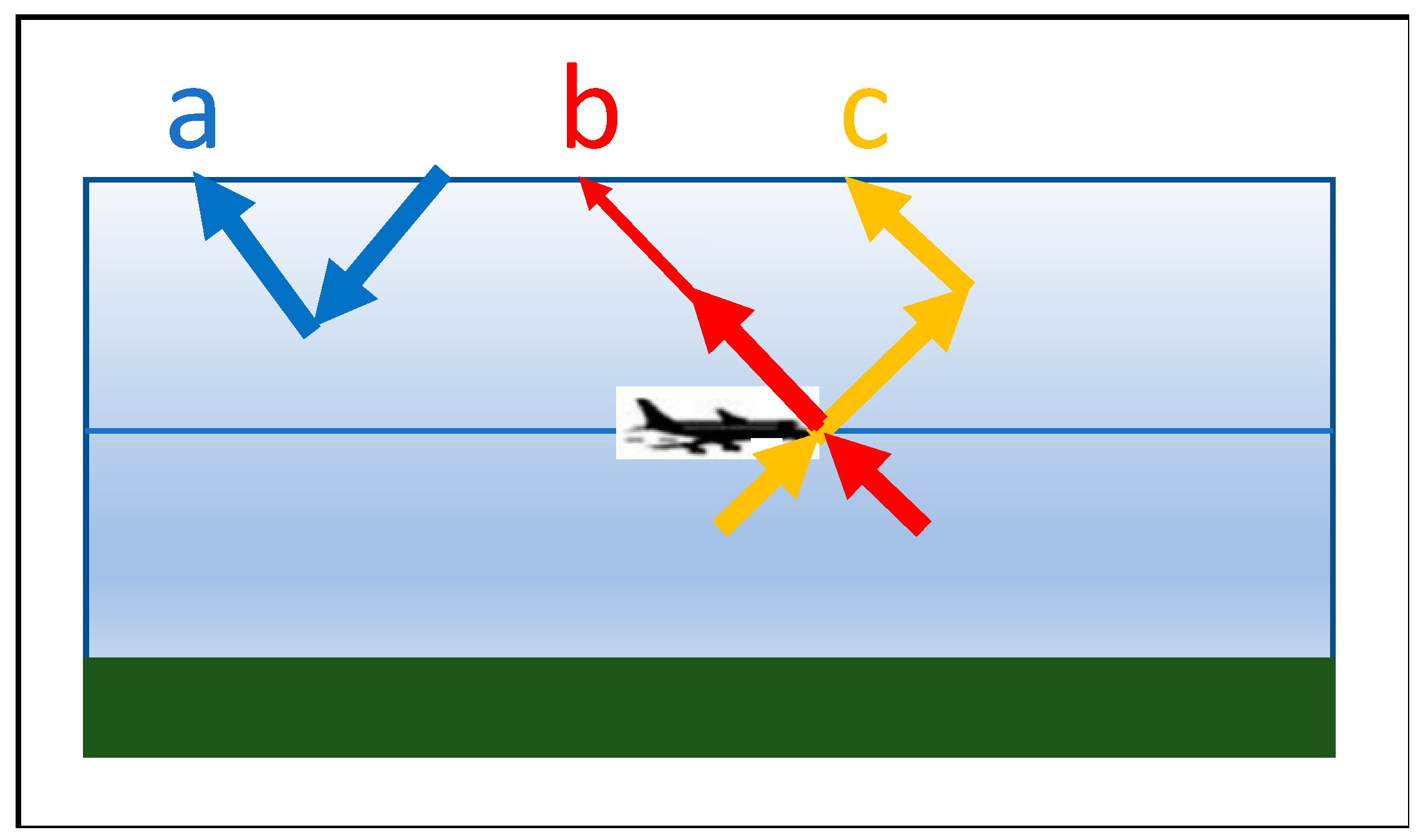
ARCTAS was an extensive NASA airborne field campaign to investigate the chemistry of the Arctic’s lower atmosphere [21]. Flights were based in Alaska during April 2008 and in western Canada during June and July 2008. The primary goal of ARCTAS was to better understand the factors driving current changes in Arctic atmospheric composition and climate, including (1) transport of mid-latitude air pollution, (2) boreal forest fires, (3) aerosol radiative forcing, and (4) chemical processes.

In this study, we focus on deriving angular distribution models for smoke-laden atmospheric columns using unique multiangular-multispectral measurements from CAR observations and radiative transfer simulations. Such ADMs are needed to convert the radiance measurements at a given Sun–satellite geometry to outgoing reflected solar radiative fluxes [9].

The CAR instrument was flown aboard the NASA P-3B aircraft, whose payload included 10 primary instruments for measuring aerosol optical depth, aerosol extinction and scattering, aerosol size distribution [22,23], solar spectral (0.380–2.200 µm) downwelling and upwelling irradiance [24], broadband downwelling and upwelling solar (0.2–3.6 µm) and IR (4.5–42 µm) irradiance [25] (http://airbornescience.nasa.gov/instrument/BBR), angular distribution of scattered radiation [19,26], cloud condensation nuclei [27,28], and NO₂ and carbon monoxide [29,30]. The base meteorological and navigational measurements were provided by the Project Data System, which was the primary navigational data system for P-3B investigators [31]. CAR data are the primary dataset for this investigation; when necessary, they are analyzed in synergy with other coincident datasets. Specifically, we also use above-aircraft aerosol optical properties from the Ames Airborne Tracking Sunphotometer (AATS) [32], in-situ aerosol single scattering albedo and particle size observations from the Particle Soot Absorption Photometer (PSAP) [33], and surface parameters from the Moderate Resolution Imaging Spectroradiometer (MODIS).

CAR is an airborne multiwavelength scanning radiometer designed to operate from various aircraft platforms (Figure 1; [19]). It has a unique design with a wide field of regard (190°) and a small instantaneous field of view (1°), which allows it to scan in a plane perpendicular to the direction of flight and provides views of the Earth-atmosphere scene from zenith to nadir on the right side of the aircraft. Data are always sampled simultaneously and continuously for 8 spectral bands from 0.34 to 1.27 µm (0.34, 0.38, 0.47, 0.68, 0.87, 1.04, 1.22, 1.27 µm) plus for one of the six bands on a filter wheel (1.66 µm for the flight analyzed here).

CAR data are stored and distributed in netCDF format by the NASA Earth Observing System Data and Information System (EOSDIS). The data used in this study are available at https://disc.gsfc.nasa.gov/datasets/CAR_ARCTAS_L1C_V1/summary. Each data file contains calibrated Earth and/or sky view measurements. For each CAR band, the data are formatted in a polar coordinate system, where the viewing zenith angles range from 0–180° in half-degree intervals, and the relative azimuth angles range from 0–360°, in 1° intervals. Thus, zenith angles of 0° and 180° represent looking straight down and straight up, respectively, and azimuths of 0° (or 360°) and 180° represent forward scattering and back scattering, respectively.

For over three decades, the CAR instrument has been used for measuring the angular distribution of reflected solar radiation of natural ecosystems worldwide in multiple campaigns [19]. These measurements have been used to derive the spectral and angular distribution of reflectance (bidirectional reflectance factor, or BRF) at the full range of zenith and azimuth angles, and thus are valuable for assessing the accuracy of satellite-derived angular models, surface bidirectional reflectance distribution functions, and atmospheric corrections [19,34,35].

CAR’s radiometric performance is well characterized [36], which allows the instrument to be used for satellite calibration/validation activities as well.

This study analyzes CAR data collected during Flight #2016 [37]. The data examined here was collected over Saskatchewan, Canada (57.06°N, 104.78°W) on June 30, 2008, around 22:45–22:48 UTC (local time: 15:45–15:54) as the aircraft circled above a smoke plume at an altitude of 5380 m. The surface elevation was ~500 m and the solar zenith angle was 53°. Figure 2 shows the smoke plumes observed from a satellite and from the aircraft.

2.2. Simulations

This study analyzes CAR observations using radiative transfer simulations performed using the libRadtran Version 2 radiative transfer simulation package [38,39], which is publicly available at http://www.libradtran.org.

The simulations are carried out using the Discrete Ordinates Radiative Transfer (DISORT) solver included in libRadtran. The calculations include correlated-k spectral integration using k-values from libRadtran’s Kato2 table for shortwave broadband simulations (an optimized version of the k-values in [40]), and the reptran table for single CAR band simulations. The libRadtran simulations are set up to provide flux values as well as radiances at 10° angular resolution; these radiances are then interpolated to the 1° resolution of CAR measurements.

The simulations assume a cloud-free subarctic summer atmosphere. We note that, as can be seen in Figure 1b, some clouds were embedded in the observed smoke plume. As it will be highlighted in Section 3.2, the embedded clouds affected the observations and the derived ADMs for some very oblique view directions; this is one reason why very oblique views were not used in the smoke parameter estimations discussed in Section 3.1. More generally, the radiative impact of clouds in CAR smoke observations during ARCTAS has been analyzed in [41].

In performing the simulations, we assume a bimodal aerosol size distribution that includes both the accumulation mode and the coarse mode of the MODIS Collection 6 absorbing/smoke land aerosol model in Table 1 of [42]. As noted in [42], this aerosol model was developed to represent aerosols from forest/vegetation fires and developing industrial regions. About 10 minutes before the CAR observations were taken, the P-3B aircraft passed through a smoke plume and the Particle Soot Absorption Photometer (PSAP) instrument reported 530–550 nm single scattering albedos around 0.89 and submicron fractions around 0.82—which, for the MODIS smoke models, implies a coarse mode fraction of 0.18. As discussed below in Section 3.1, this study estimates aerosol optical depth (AOD) and wavelength-dependent single scattering albedo (SSA) by minimizing the differences between simulations and CAR observations.

The simulations assume that the smoke layer was between 0.5–4.5 km altitudes above the surface. While the plume base was not seen from CAR as the P-3B aircraft did not enter the plume right near the location of analyzed CAR observations, the 500 m base altitude appears to be a reasonable estimate: About 45 minutes before the CAR observations analyzed here were taken, the P-3B aircraft flew through a plume at around 700 m altitude, revealing that the plume base was below 700 m. Brief sensitivity tests indicated that small changes in smoke base altitude would not significantly impact the results presented here.

In considering aerosols above the aircraft, the simulations assume non-absorbing particles with scattering properties similar to those of smoke. While this may be a questionable assumption, the impact of uncertainties should be quite small, as the aerosol layer above the aircraft was very thin. Specifically, coincident measurements from the AATS onboard the aircraft indicated that the above-aircraft AOD was 0.017 at 500 nm.

In addition, the calculations simulate surface reflection using the Ross-Thick-Li-Sparse (RTLS) model [11]. The initial estimates of input parameters for this model at seven visible and near-infrared wavelengths are obtained from the MODIS land product MCD43C1 [43]. Parameters at these seven MODIS wavelengths are then interpolated/extrapolated to cover the entire solar spectrum at a high spectral resolution (2 or 20 nm at wavelengths shorter or longer than 800 nm, respectively). This interpolation/extrapolation forces the spectral variations between two MODIS wavelengths to follow the shape of conifer albedo spectral variations in the ASTER spectral library (http://speclib.jpl.nasa.gov; [44]) at the library’s (2 or 20 nm) spectral resolution.

3. Results and Discussions

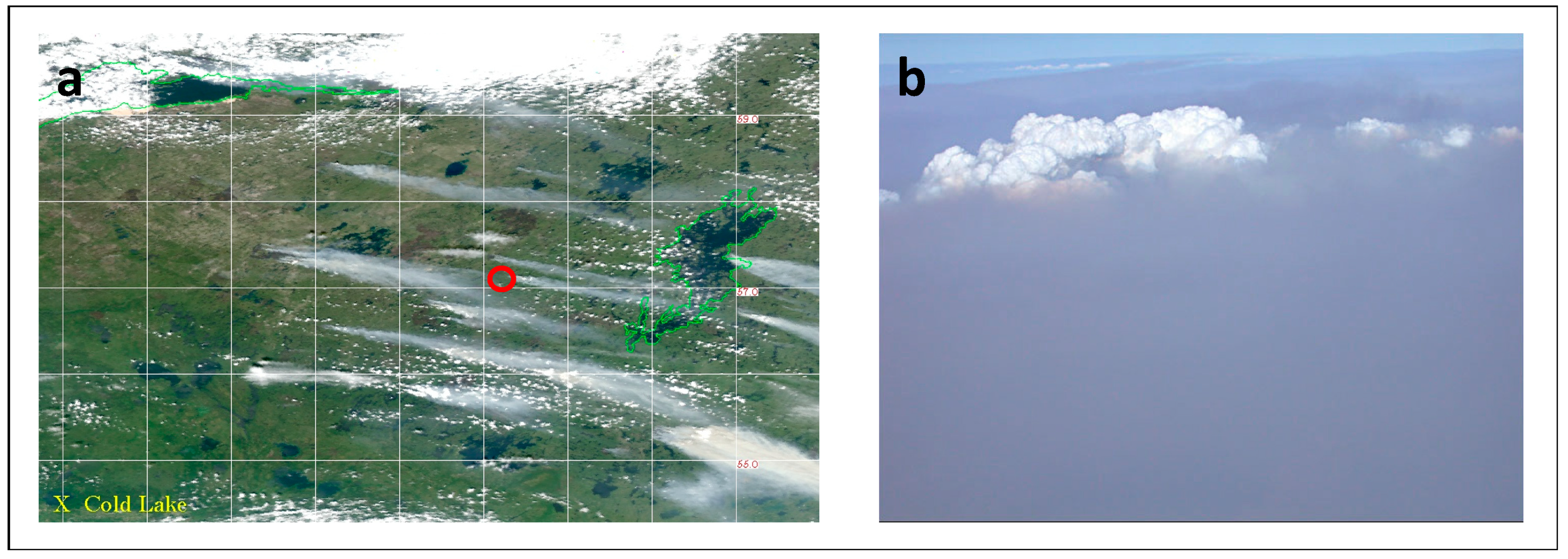
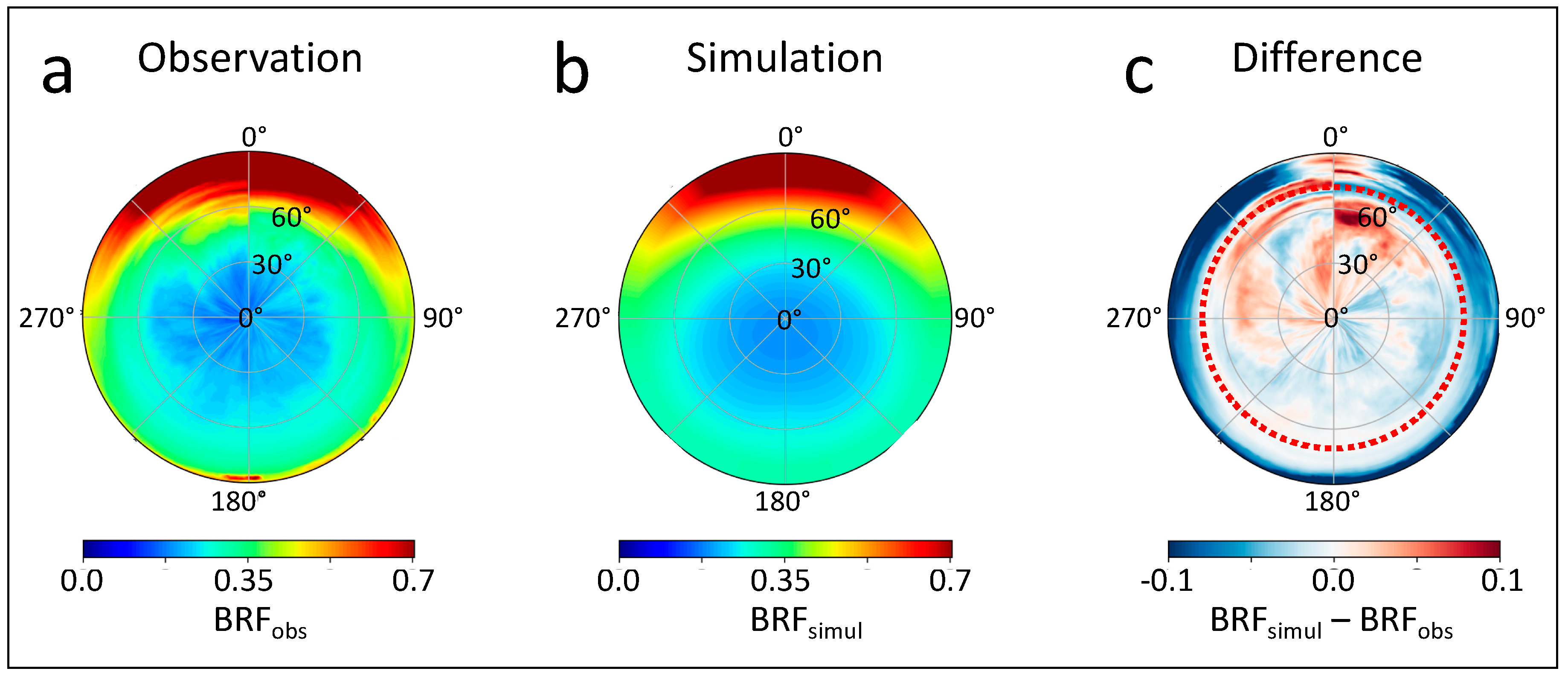
3.1. Scene Characterization

This study aims at characterizing broadband TOA ADMs by taking advantage of the information content of multiangle, multispectral CAR measurements. Connecting observations available at discrete wavelengths to broadband fluxes inherently requires radiative transfer simulations. The previous section described some aspects of these simulations; here we discuss additional scene characterization that was needed to facilitate realistic broadband simulations. The goal here is to obtain a realistic set of aerosol parameters that we will then vary as we develop statistical relationships between CAR spectral and TOA broadband ADMs. Since we will perturb the scene parameters anyway, pinning down the exact values of aerosol optical depth and absorptivity is less critical in this particular study. We note, however, that in a recent study, CAR data was used to explore the benefits of multiangle observations for estimating scene albedos and surface parameters such as NDVI [20].

The most important goal of our scene characterization effort is to estimate the optical depth of the observed smoke plume. AOD retrievals are available for the MODIS Aqua image taken about two hours before the CAR observations, but CAR retrievals of aerosols are important because AOD can vary sharply in fresh smoke plumes. In addition to AOD, we also estimate the absorptivity of smoke particles. This is important because we analyze CAR measurements taken about 10 minutes after PSAP provided information on smoke absorption—and that information came from a different location, where smoke may have had a somewhat different age and radiative properties. The adjustments of PSAP absorptivity values can also help mitigate the impact of PSAP absorption measurement uncertainties, which are about 20% according to the PSAP data file.

Overall, CAR-based retrievals provide three smoke parameters: AOD at 550 nm, single scattering albedo at 550 nm, and the slope (S) that characterizes the wavelength-dependence of single scattering albedo through

$$SSA\left(\lambda \right)=SS{A}_{550nm}+\left(SS{A}_{\lambda }^{\mathrm{Mie}}-SS{A}_{550\mathrm{nm}}^{\mathrm{Mie}}\right) S,$$

(1)

where λ is wavelength in nm and SSA^Mie is the single scattering albedo of the used MODIS aerosol model. The slope parameter, S, allows us to adjust the steepness of the SSA wavelength dependence, which is important because earlier studies found this steepness to be quite different for different smoke plumes [45,46,47]. We note that, in essence, Equation (1) uses the MODIS aerosol model as a source of a priori information on the spectral shape of the SSA(λ) function, and then it adjusts this shape using S in order to best fit the CAR observations.

The retrievals estimate the AOD, SSA, and S values that allow libRadtran simulations (see Section 2.2) to best match the bidirectional reflectance factor (BRF) values observed by CAR. Following the notations in [19], BRF is defined here as

$$BRF\left(\lambda ,\theta ,\phi \right)=\frac{\pi I\left(\lambda ,\theta ,\phi \right)}{{\mu }_0 F_0},$$

(2)

where I is radiance [W/m²/µm/sr], $\theta$ and $\phi$ are the viewing zenith and azimuth angles, µ₀ is the cosine of the solar zenith angle, and F₀ is the extraterrestrial solar irradiance [W/m²/µm]. Observed and simulated BRFs are compared at 380 and 470 nm wavelengths, where smoke has a strong impact and the underlying surface is dark (ensuring that surface variability does not cause large retrieval uncertainties). The comparison considers BRFs for viewing zenith angles less than 70°; more oblique observations are not used in order to limit any complications due to horizontal variations in smoke and surface properties and to avoid the effects of clouds observed at very oblique angles (Figure 1b and Section 3.2).

The retrievals found that libRadtran simulations best match the CAR observations for AOD_550nm = 3.9, SSA_550nm = 0.90, and S = 1.0. As an illustration, Figure 3 shows the angular distribution of the observed and the best matching simulated BRFs at 470 nm. The figure shows that the simulations capture the dominant patterns of observed angular variations, although they slightly overestimate oblique values near the solar plane and underestimate sideways reflection. We note that our estimates of aerosol parameters have significant uncertainties, as the root-mean-square (RMS) error between the observations and simulations remains below the 5% level of CAR calibration uncertainty if AOD is between 3.5 and 8, and SSA is between 0.893 and 0.905. (The range extends to such high AODs because of the weak sensitivity of reflectance to optical depth in such thick and absorbing plumes.) Regardless of the exact value of the AOD, we can say confidently that the observed smoke layer had a dramatic impact on solar radiation: The simulated overall shortwave radiative forcing for the best-estimate aerosol parameters (AOD = 3.9, SSA = 0.9, S = 1) are 73 W/m² and 460 W/m² at the top of the atmosphere and the surface, respectively, with these values varying by only a few and a few dozen W/m² within the range of retrieval uncertainty. We reiterate, however, that the main goal of our retrievals is not to pin down exactly the smoke properties, but to obtain base values around which we will perturb scene parameters when we develop statistical relationships between CAR data and broadband TOA BRFs (in Section 3.2).

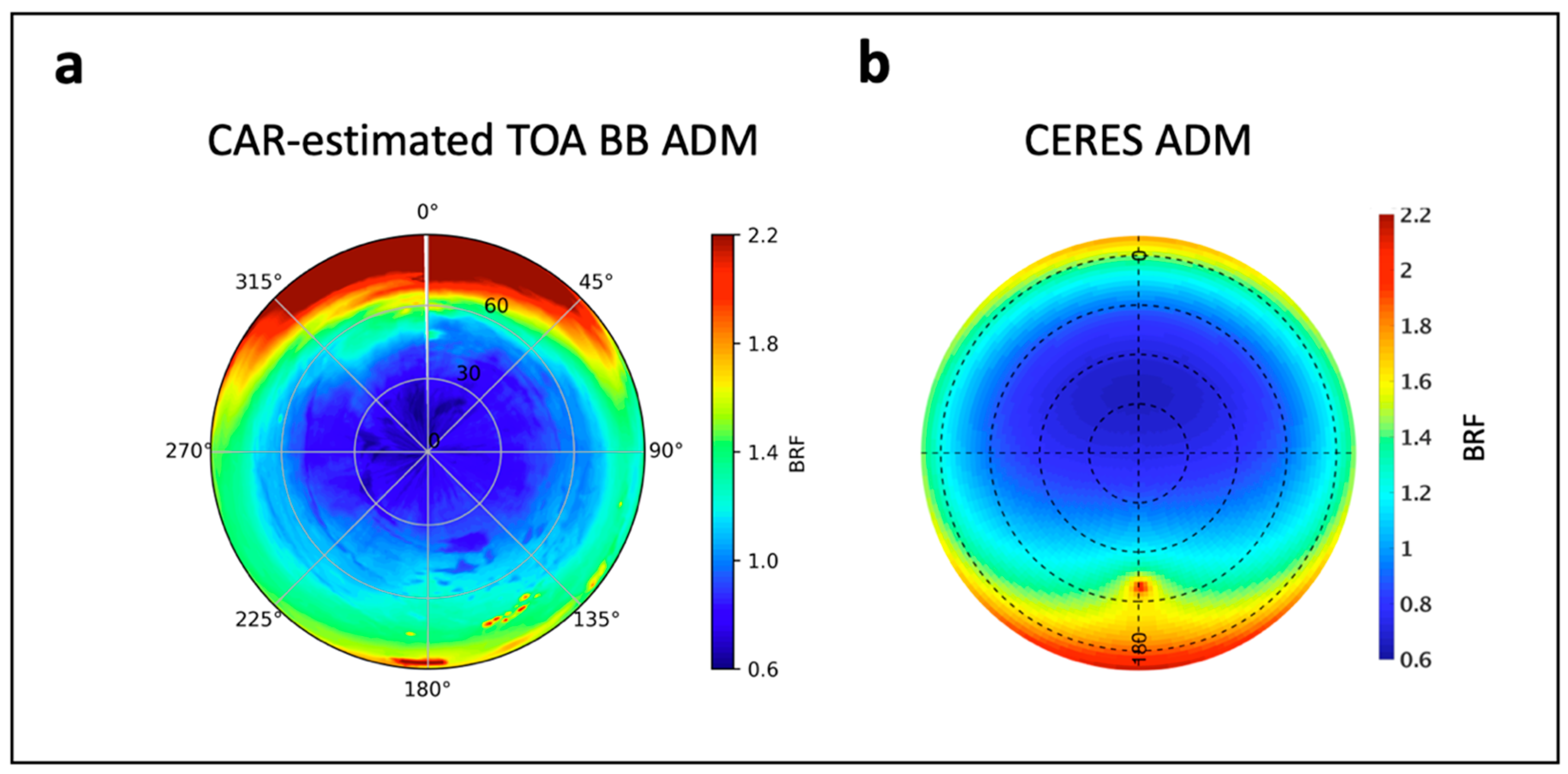
3.2. Broadband Top-of-Atmosphere Angular Model

As mentioned in the introduction, the main purpose of this study is to explore the usage of airborne CAR measurements for deriving and examining broadband angular models at the top of the atmosphere. Such TOA models are used, for example, in satellite studies of the Earth radiation budget [8,9,10].

Obtaining TOA broadband ADMs based on CAR observations involve two tasks: estimating the radiative effects of the atmosphere above the aircraft, and filling the gaps between CAR wavelengths. In other words, the two tasks are: (a) conversion from aircraft altitude to TOA, and (b) narrowband to broadband conversion.

We carry out these two tasks by combining them into a single linear regression—an approach that has been successfully used in earlier studies for narrowband-to-broadband conversions [48,49]. Our initial calculations use the equation

$$BR{F}_{BB}^{TOA}\left(\theta ,\phi \right)={{\displaystyle \sum }}_{i=1}^{N_{\lambda }}[a\left(\theta ,\phi \right)+b_i\left(\theta \right)·BR{F}_i^{CAR}\left(\theta ,\phi \right)+c_i\left(\theta \right)F_i^{\uparrow CAR}],$$

(3)

where N_λ is the number of CAR spectral bands (= 9), while a, b, and c are regression coefficients (discussed below). $BR{F}_i^{CAR}$ values are calculated from the CAR-observed radiances using Equation (2), and the $F_i^{\uparrow CAR}$ upwelling flux values are obtained from these $BR{F}_i^{CAR}$ values through angular integration. As illustrated in Figure 4, the three terms on the right side can account for (a) the effect of reflection by atmospheric layers above the aircraft (b) attenuation of CAR-observed upwelling radiation above the aircraft, and (c) atmospheric scattering above the aircraft that redirects the upwelling radiation observed by CAR into the direction $\left(\theta ,\phi \right)$. We note that term a is related to the path radiance used in earlier studies [50], but in our case, this term includes only the effects of the atmosphere above the aircraft and cannot be directly observed by itself. Instead, the values of $a\left(\theta ,\phi \right)$ are obtained through libRadtran simulations assuming a thick, fully absorbing aerosol layer at aircraft altitude (with input AOD_550nm = 10, SSA_550nm = 0.0, S = 0.0).

Let us mention that, instead of combining our two tasks—atmospheric correction and narrowband-to-broadband conversion—into a single-step regression, one could use radiative transfer modeling for the first step and use regression only for the second step. A such two-step approach would be more complex but also more accurate, as it would not use the assumption that radiance enhancement by scattering above the aircraft (process c in Figure 5 and the last term in Equation (3)) depends only on the amount and not the angular distribution of upwelling radiation. However (as it will be discussed in the second paragraph of Section 3.3), in our case the relative error of our single-step regression approach is only about 0.3% for the atmospheric correction and narrowband-to-broadband conversions combined. Therefore, using a more accurate method for the atmospheric correction part of our task could provide only small (< 0.3%) benefits in return for the added complexity. However, we need to keep in mind that the benefits may become more significant in case of more anisotropic radiance fields, for example for very low sun.

In practice, the calculation of regression is performed by dividing the solar spectrum into 9 intervals centered around each CAR wavelength, and then estimating broadband TOA BRFs as a sum of BRF integrals over each spectral interval (${\widehat{BRF}}_i^{TOA})$:

$$BR{F}_{BB}^{TOA}\left(\theta ,\phi \right)={{\displaystyle \sum }}_{i=1}^{N_{\lambda }}{w}_i{\widehat{BRF}}_i^{TOA}\left(\theta ,\phi \right)={{\displaystyle \sum }}_{i=1}^{N_{\lambda }}{w}_i\left(a_i\left(\theta ,\phi \right)+b_i\left(\theta \right)·BR{F}_i^{CAR}\left(\theta ,\phi \right)+c_i\left(\theta \right)F_i^{\uparrow CAR}\right),$$

(4)

where w_i tells what fraction of the total TOA solar irradiance lies within the i^th spectral interval (${{\displaystyle \sum }}_{i=1}^{N_{\lambda }}{w}_i=1$).

As mentioned in Section 3.1, the b_i($\theta$), and c_i($\theta$) regression coefficients in Equation (3) were determined through linear regression over simulated BRF values. In particular, 100 triplets of libRadtran simulations were performed, yielding ${\widehat{BRF}}_i^{TOA}, BR{F}_i^{CAR}, \mathrm{and} F_i^{\uparrow CAR}$ values for 100 scenes. The simulations used the parameters described in Section 3.1, except that for each of the 100 scenes, five of the scene parameters had values chosen from uniform random distributions within the following ranges (centered around our best-guess estimates of scene parameters): 2 ≤ AOD_550nm ≤ 6, 0.89 ≤ SSA_550nm ≤ 0.91, 0 ≤ S ≤ 2, 0 ≤ f_sfc ≤ 2, and 0.136 ≤ CMF ≤ 0.236. Here, f_sfc is a factor by which all parameters of the Ross Thick Li Sparse model (Section 2.2) are multiplied to represent surface variability, and CMF is the aerosol coarse mode fraction.

Figure 5 shows the azimuthally averaged values of the coefficients a_i$\left(\theta ,\phi \right)$ obtained from libRadtran simulations, and the b_i($\theta$) and c_i($\theta$) coefficients obtained through regression for the 100 scenes. Panel a shows that coefficient a decreases toward longer wavelengths and smaller viewing zenith angles (that is, shorter optical paths) due to the weaker Rayleigh scattering by the air above the aircraft.

Panel b shows that at shorter wavelengths (Bands 1–4), b-values increase with wavelength, as Rayleigh scattering by the air above CAR gets weaker. At longer wavelengths, however, Rayleigh scattering is already very weak and further weakening does not make much of a difference. Instead, at those wavelengths, the spectral dependence of b-values is influenced mostly by absorption above the aircraft: For example, the values for Band 6 centered around 1040 nm are so high because there is very little Rayleigh scattering and gaseous absorption in the 6th spectral interval ranging from 955 nm to 1100 nm (e.g., [51]; https://commons.wikimedia.org/wiki/File:Solar_Spectrum.png). The figure also shows that for the most part, coefficient b decreases with increasing viewing zenith angle for the UV-VIS bands, as the transmission through the air above the aircraft gets smaller for longer, more oblique paths. At longer wavelengths near nadir, however, the b-values increase with viewing zenith angle. This is because the b and c values are estimated through a regression that may be influenced by nonlinearities and by inherent correlations between the $BR{F}_i^{CAR} \mathrm{and} F_i^{\uparrow CAR}$ values (that are multiplied in Equation (4) by b and c, respectively). We note that we can avoid this hard-to-physically-interpret increase in b by setting the c-values to zero, but this would result in a significant (> 30%) increase in the RMS error of the regression for the 100 scenes.

Figure 5c shows that as b drops near nadir at long wavelengths, c increases in compensation. The figure also shows that, apart from this compensatory increase, c-values tend to increase at shorter wavelengths and more oblique views due to the stronger Rayleigh scattering and longer optical paths. Finally, we note that the compensatory behavior of b and c implies that each of the two coefficients represents not a single process, but a combination of the red (extinction) and yellow (enhancement) processes in Figure 4.

Figure 6a shows the TOA broadband ADMs estimated by applying Equation (4) to the CAR observations, and then applying the definition of ADMs

$$ADM\left(\theta ,\phi \right)=\frac{BRF\left(\theta ,\phi \right)}{{{\displaystyle \int }}_{2\pi }^{}cos\left({\theta }^{\prime }\right)BRF\left({\theta }^{\prime },{\phi }^{\prime }\right)d{\phi }^{\prime }d{\theta }^{\prime }}$$

(5)

where the denominator is the upward flux (calculated as the weighted integral of BRF values over the down-looking hemisphere). Following the pattern of CAR observations (e.g., Figure 3a), the estimated ADM values increase for oblique view directions, with an especially strong increase in the forward direction (due to a forward peak in the smoke particle scattering phase function). In addition, Figure 6a also displays behaviors not present in Figure 3a: a smaller peak in the backscattering direction and well-pronounced small-scale patterns in less oblique directions. These features are caused by the vegetated surface hotspot and by spatial variations in surface type, which can influence TOA reflectance at the longer wavelengths where Rayleigh scattering and smoke effects are weak. In addition, the effects of small bright clouds embedded into the smoke layer (see Figure 1b) appear at very oblique view directions around 150° azimuth.

In turn, Figure 6b shows the CERES TOA broadband clear sky ADM most applicable to the scene observed by CAR. This is the monthly mean ADM for the 1° by 1° area located over the CAR scene that was developed using CERES rotating azimuth plane observations taken between 2000 and 2004 on Terra spacecraft. Over land, clear-sky reflectance measured by the CERES instruments over each 1° latitude by 1 ° longitude for every calendar month were stratified by NDVI (measured at TOA) and cosine of viewing zenith angle. For each stratification, the modified Ross-Li fit [52] was used to characterize the TOA anisotropy [10]. The stratification by TOA NDVI was intended to capture the anisotropy variations as the aerosol loading changes, as greater TOA NDVI corresponding to smaller AOD and vice versa. The aerosol loading during the period used to develop the ADM was much smaller (AOD at 550 nm on the order of 0.1–0.2) than in the case considered here. Thus, the CERES ADM is different from the ADM derived for this thick smoke plume case (AOD at 550 nm is 3.9).

We note that due to the high optical depth of the observed smoke plume, the CAR ADM in Figure 6a is actually more similar to CERES thin cloud ADMs than to the CERES clear-sky ADM in Figure 6b. For example—even though the markedly smaller size and stronger absorptivity of smoke particles cause significant differences between smoke and cloud reflection—both the CAR smoke and CERES cloud ADMs have the largest values in forward (and not back) scattering directions. In turn, the CERES clear-sky ADM in Figure 6b is more similar to CAR observations collected over forests on days with low aerosol loading (e.g., Figure 6c of [19]): In both cases, the dominance of surface reflection causes the largest values to appear at back scatter directions.

3.3. Sensitivity of the Angular Model to Variations in Scene Parameters

The differences between Figure 6a,b illustrate the fact that ADMs can vary substantially with surface and atmospheric conditions. This raises two questions: What is the uncertainty of the ADM in Figure 6a, and how applicable is this ADM for other cases of wildfire smoke?

We characterize the uncertainty of the ADM in Figure 6a through the uncertainty of the regression used for deriving it. Specifically, we compare the accurate, libRadtran-simulated TOA broadband ADMs of our 100 scenes (see Section 3.2) to the regression-estimated ADMs we get by applying Equations (4) and (5) to the same 100 scenes. The mean absolute value of the difference is 0.003, indicating that the uncertainty is quite low as long as the scene parameters remain within the ranges considered in the 100 scenes (for example, AOD is between 2 and 6). We note, however, that this estimate does not include the effects of assumptions that were constant for all 100 scenes, for example the assumption of an average subarctic summer humidity profile.

To gauge how applicable the CAR-based ADM in Figure 6a is for other, satellite-observed smoke plumes, we next examine libRadtran-simulated TOA broadband ADMs. In particular, we check how the ADMs change if we vary the 5 scene parameters that were considered in obtaining the regression coefficients a, b, and c (in Section 3.2): AOD_{550 nm}, SSA_{550 nm}, S, f_sfc, and CMF. When varying the parameters one-by-one, the results show that the RMS change in ADM values (specified for each view direction at a 1° angular resolution) remains below 1% within the following parameter ranges: 3 < AOD_{550 nm} < 6, 0.888 < SSA_{550 nm} < 0.912, 0.2 < S < 2.7, 0.3 < f_sfc < 4.5, and 0.13 < CMF < 0.28.

We note that the wide range for variations in f_sfc may not only encompass variations in forest albedo, but may also allow applying this ADM to smoke plumes over surfaces other than coniferous forests (such as deciduous forests, or other—especially vegetated—dark surfaces). One possibility for testing whether the ADM could be used in a particular region would be to compare its RTLS parameters (e.g., from the MODIS MCD43C1 product) to those of the ARCTAS area: Are the ratios of corresponding RTLS parameters of the two areas within the f_sfc range that implies a 1% RMS change in the ADM (0.3–4.5)?

It is also important to consider whether CAR-based ADMs can be applied to satellite observations taken at slightly different solar elevations. LibRadtran simulations based on the smoke parameters estimated in Section 3.1 show that if the solar zenith angle changes from the 53° of CAR observations to 50° (of hypothetical satellite observations), the RMS change in ADM values is 2.8%. Fortunately—unlike scene parameters—the solar zenith angle is usually well known. This raises the possibility of estimating what $BR{F}_{BB,CAR}^{TOA}$ (the CAR-based TOA broadband BRFs needed to get ADMs) would be for slightly different solar elevations:

$$BR{F}_{BB,CAR}^{TOA}\left(\theta ,\phi ,{\theta }_0^{sat}\right)= BR{F}_{BB,CAR}^{TOA}\left(\theta ,\phi ,{\theta }_0^{CAR}\right)\frac{BR{F}_{BB,simul}^{TOA}\left(\theta ,\phi ,{\theta }_0^{sat}\right)}{BR{F}_{BB,simul}^{TOA}\left(\theta ,\phi ,{\theta }_0^{CAR}\right)},$$

(6)

where ${\theta }_0^{sat}$ and ${\theta }_0^{CAR}$ are the solar zenith angles of satellite and CAR observations, and $BR{F}_{BB,simul}^{TOA}$ is the TOA broadband BRF simulated by libRadtran for the scene parameters estimated in Section 3.1. The usefulness of Equation (6) can be characterized through libRadtran simulations. For this, we first simulated $BR{F}_{BB,CAR}^{TOA}\left(\theta ,\phi ,{\theta }_0^{CAR}\right)$ values using the scene parameters estimated in Section 3.1. We then simulated $BR{F}_{BB,simul}^{TOA}\left(\theta ,\phi ,{\theta }_0^{sat}\right)$ and $BR{F}_{BB,simul}^{TOA}\left(\theta ,\phi ,{\theta }_0^{CAR}\right)$ values for a lower AOD (2.1 instead of 3.9, a drop that caused a 3% RMS change in ADM values). We then used these BRFs in Equation (6) to estimate $BR{F}_{BB,CAR}^{TOA}\left(\theta ,\phi ,{\theta }_0^{sat}\right)$, and then used Equation (5) to get the corresponding ADM values. This yielded a modified CAR-based ADM, whose RMS difference from the exact ADM (obtained through libRadtran simulations for ${\theta }_0^{sat}$) was less than 0.5% (instead of the original 2.8%).

Finally, let us combine our individual estimates by assuming that the five considered scene parameters and the solar elevation vary independently within the ranges mentioned above (e.g., 3 < AOD < 6, 50° < $\theta$₀ < 56°). Since individual variations in each parameter cause 1% RMS change in ADM values (or 0.5% for $\theta$₀), we estimate that CAR can provide ADMs applicable to satellite observations with an RMS uncertainty of $\sqrt{5\ast 1^2+{0.5}^2}\%=\sqrt{5.25}\%\approx 2.3\%$. An overview of the sensitivity results is presented in

Table 2. Ranges for scene parameter variations causing 1% root-mean-square (RMS) deviations from the estimated smoke ADM shown in Figure 6a. If individually, independent variations in each parameter cause 1% deviation, the total RMS deviation will be 2.3%. The used regression method adds another 0.3% uncertainty to the estimated ADM.

Parameter	Range
AOD550 nm	3–6
SSA550 nm	0.888–0.912
S	0.2–2.7
fsfc	0.3–4.5
CMF	0.13–0.28
SZA	50°–56°1

¹ Range causing 0.5% ADM change.

.

4. Conclusions

This study examined the angular distribution of sunlight reflected from a wildfire smoke plume that was observed over boreal forests in Canada during the ARCTAS campaign. The study characterized this angular distribution using multiangular, multispectral observations by the Cloud Absorption Radiometer (CAR) that were taken from an aircraft that circled above the plume. The study combined CAR observations with data from other airborne and satellite instruments (AATS, PSAP, MODIS) to constrain possible scene properties, and with radiative transfer simulations to interpret the observations.

First, the study estimated some key radiative properties of the observed smoke plume. An iterative procedure was used to find the smoke parameters that allow simulations to best match all CAR observations with a viewing zenith angle less than 70°. The best-estimate result from this procedure was a 550 nm aerosol optical depth of 3.9 and single scattering albedo of 0.9.

Next, the paper developed a technique to use the narrowband observations that were taken from an aircraft flying about a kilometer above the smoke layer and estimate the broadband TOA radiances a satellite instrument such as CERES would have observed. This regression-based technique included both an atmospheric correction for the impacts of the atmosphere above the aircraft and a narrowband-to-broadband conversion. The empirical regression coefficients needed for this technique were determined through radiative transfer simulations in which the estimated parameters of the smoke plume were perturbed randomly. The calculated ADM was found to be substantially different from the monthly average ADM used in the operational data processing of CERES observations over the same area. The magnitude of the difference depends on view direction, but it typically changes the estimated radiative flux values by dozens of percent. The CERES ADM is so different because it was constructed using data collected under much lower aerosol optical depth conditions than the thick plume case considered here.

Finally, a sensitivity analysis showed that the estimated ADM remains accurate for a reasonably wide range of smoke and (forested) surface parameters and solar elevations. This implies that a full ADM derived using multi-angular and multi-spectral airborne observations of the angular distribution of scattered radiation could help improve the accuracy of radiative flux estimates that are based on broadband satellite observations over a fairly wide range of (forested) surface, atmospheric, and illumination conditions.

Overall, the results are expected to help improve satellite-based estimates of the radiative effect of wildfire smoke. This, in turn, can lead to more realistic treatment of wildfire smoke in climate simulations. Given the significant radiative impact of smoke and the observed and foreseen increasing frequency of wildfires, the results can, ultimately, contribute to improving the accuracy of climate predictions.

References

1. Mouillot, F.; Narasimha, A.; Balkanski, Y.; Lamarque, J.F.; Field, C.B. Global carbon emissions from biomass burning in the 20th century. Geophys. Res. Lett. 2006, 33, L01801. [Google Scholar] [CrossRef]
2. Marlon, J.R.; Bartlein, P.J.; Carcaillet, C.; Gavin, D.G.; Harrison, S.P.; Higuera, P.E.; Joos, F.; Power, M.J.; Prentice, I.C. Climate and human influences on global biomass burning over the past two millenia. Nat. Geosci. 2008, 1, 697–702. [Google Scholar] [CrossRef]
3. Spracklen, D.V.; Mickley, L.J.; Logan, J.A.; Hudman, R.C.; Yevich, R.; Flannigan, M.D.; Westerling, A.L. Impacts of climate change from 2000 to 2050 on wildfire activity and carbonaceous aerosol concentrations in the western United States. J. Geophys. Res. 2009, 114, D20301. [Google Scholar] [CrossRef]
4. Kloster, S.; Mahowald, N.M.; Randerson, J.T.; Thornton, P.E.; Hoffman, F.M.; Levis, S.; Lawrence, P.J.; Feddema, J.J.; Oleson, K.W.; Lawrence, D.M. Fire dynamics during the 20th century simulated by the Community Land Model. Biogeosciences 2010, 7, 1877–1902. [Google Scholar] [CrossRef] [Green Version]
5. Pechony, O.; Shindell, D.T. Driving forces of global wildfires over the past millennium and the forthcoming century. Proc. Natl. Acad. Sci. USA 2010, 107, 19167–19170. [Google Scholar] [CrossRef] [Green Version]
6. IPCC. Climate Change 2013: The Physical Science Basis. Contribution of Working Group I to the Fifth Assessment Report of the Intergovernmental Panel on Climate Change; Stocker, T.F., Qin, D., Plattner, G.-K., Tignor, M., Allen, S.K., Boschung, J., Nauels, A., Xia, Y., Bex, V., Midgley, P.M., Eds.; Cambridge University Press: Cambridge, UK; New York, NY, USA, 2013; p. 1535. [Google Scholar] [CrossRef]
7. Wielicki, B.A.; Barkstrom, B.R.; Harrison, E.F.; Lee, R.B.; Smith, G.L.; Cooper, J.E. Clouds and the Earth’s Radiant Energy System (CERES): An earth observing system experiment. Bull. Am. Meteorol. Soc. 1996, 77, 853–868. [Google Scholar] [CrossRef]
8. Loeb, N.G.; Parol, F.; Buriez, J.C.; Vanbauce, C. Top-of-atmosphere albedo estimation from angular distribution models using scene identification from satellite cloud property retrievals. J. Clim. 2000, 13, 1269–1285. [Google Scholar] [CrossRef]
9. Loeb, N.G.; Kato, S.; Loukachine, K.; Manalo-Smith, N. Angular distribution models for top-of-atmosphere radiative flux estimation from the Clouds and the Earth’s Radiant Energy System instrument on the Terra satellite. Part I: Methodology. J. Atmos. Ocean. Technol. 2005, 22, 338–351. [Google Scholar] [CrossRef]
10. Su, W.; Corbett, J.; Eitzen, Z.; Liang, L. Next-generation angular distribution models for top-of-atmosphere radiative flux calculation from CERES instruments: Methodology. Atmos. Meas. Tech. 2015, 8, 611–632. [Google Scholar] [CrossRef]
11. Lucht, W.; Schaaf, C.B.; Strahler, A.H. An algorithm for the retrieval of albedo from space using semiempirical BRDF models. IEEE Trans. Geosci. Remote Sens. 2000, 38, 977–998. [Google Scholar] [CrossRef] [Green Version]
12. Penner, J.E.; Dickinson, R.E.; O’Neill, C.A. Effects of aerosol from biomass burning on the global radiation budget. Science 1992, 256, 1432–1434. [Google Scholar] [CrossRef] [PubMed]
13. Kaufman, Y.J.; Fraser, R.S. The effect of smoke particles on clouds and climate forcing. Science 1997, 277, 1636–1639. [Google Scholar] [CrossRef]
14. Christopher, S.A.; Wang, M.; Berendes, T.A.; Welch, R.M.; Yang, S.K. The 1985 biomass burning season in South America: Satellite remote sensing of fires, smoke and regional radiative energy budgets. J. Appl. Meteorol. 1998, 37, 661–678. [Google Scholar] [CrossRef]
15. Li, X.; Christopher, S.A.; Chou, J.; Welch, R.M. Estimation of shortwave direct radiative forcing of biomass-burning aerosols using new angular models. J. Appl. Meteorol. 2000, 39, 2278–2291. [Google Scholar] [CrossRef]
16. Ramaswamy, R.; Kiehl, J.T. Sensitivities of the radiative forcing due to large loadings of smoke and dust aerosols. J. Geophys. Res. 1985, 90, 5597–5613. [Google Scholar] [CrossRef]
17. Patadia, F.; Christopher, S.A.; Zhang, J. Development of empirical angular distribution models for smoke aerosols: Methods. J. Geophys. Res. 2011, 116, D14203. [Google Scholar] [CrossRef]
18. Lyapustin, A.; Gatebe, C.K.; Kahn, R.; Brandt, R.; Redemann, J.; Russell, P.; King, M.D.; Pedersen, C.A.; Gerland, S.; Poudyal, R.; et al. Analysis of snow BRF from ARCTAS Spring-2008 campaign. Atmos. Chem. Phys. 2010, 10, 4359–4375. [Google Scholar] [CrossRef]
19. Gatebe, C.K.; King, M.D. Airborne spectral BRDF of various surface types (ocean, vegetation, snow, desert, wetlands, cloud decks, smoke layers) for remote sensing applications. Remote Sens. Environ. 2016, 179, 131–148. [Google Scholar] [CrossRef]
20. Nag, S.; Gatebe, C.K.; Hilker, T. Simulation of multiangular remote sensing products using small satellite formations. IEEE J. Sel. Top. Appl. Earth Obs. Remote Sens. 2016, 10, 638–653. [Google Scholar] [CrossRef]
21. Jacob, D.J.; Crawford, J.H.; Maring, H.; Dibb, J.E.; Clarke, A.D.; Ferrare, R.A.; Hostetler, C.A.; Russell, P.B.; Singh, H.B.; Thompson, A.M.; et al. The arctic research of the composition of the troposphere from aircraft and satellites (ARCTAS) mission: Design, execution, and first results. Atmos. Chem. Phys. 2010, 10, 5191–5212. [Google Scholar] [CrossRef]
22. Russell, P.B.; Livingston, J.M.; Hignett, P.; Kinne, S.; Wong, J.; Hobbs, P.V. Aerosol-induced radiative flux changes off the United States Mid-Atlantic coast: Comparison of values calculated from sunphotometer and in situ data with those measured by airborne pyranometer. J. Geophys. Res. 1999, 104, 2289–2307. [Google Scholar] [CrossRef]
23. Clarke, A.; McNaughton, C.; Kapustin, V.; Shinozuka, Y.; Howell, S.; Dibb, J.; Zhou, J.; Anderson, B.; Brekhovskikh, V.; Turner, H.; et al. Biomass burning and pollution aerosol over North America: Organic components and their influence on spec-tral optical properties and humidification response. J. Geophys. Res. 2007, 112, D12S18. [Google Scholar] [CrossRef]
24. Pilewskie, P.; Pommier, J.; Bergstrom, R.; Gore, W.; Howard, S.; Rabbette, M.; Schmid, B.; Hobbs, P.V.; Tsay, S.C. Solar spectral radiative forcing during the Southern African Regional Science Initiative. J. Geophys. Res. 2003, 108, 8486. [Google Scholar] [CrossRef]
25. Bucholtz, A.; Naval Research Laboratory, Monterey, CA, USA. Personal communication, 2008.
26. Gatebe, C.K.; Várnai, T.; Poudyal, R.; Ichoku, C.M.; King, M.D. Taking the pulse of pyrocumulus clouds. Atmos. Environ. 2012, 52, 121–130. [Google Scholar] [CrossRef] [Green Version]
27. Roberts, G.; Nenes, A. A continuous-flow streamwise thermal-Gradient CCN chamber for atmospheric measurements. Aerosol Sci. Technol. 2005, 39, 206–221. [Google Scholar] [CrossRef]
28. Lance, S.; Medina, J.; Smith, J.N.; Nenes, A. Mapping the operation of the DMT continuous flow CCN counter. Aerosol Sci. Technol. 2006, 40, 242–254. [Google Scholar] [CrossRef]
29. Strawa, A.W.; Provencal, R.; Owano, T.; Kirschstetter, T.W.; Hallar, G.; Williams, M.B. Aero3X: Fast, accurate measurement of aerosol optical properties for climate and air quality studies. In Proceedings of the American Geophysical Union, Fall Meeting 2007, San Francisco, CA, USA, 10–14 December 2007; abstract #A53G-03. Available online: https://ui.adsabs.harvard.edu/abs/2007AGUFM.A53G..03S/abstract (accessed on 24 June 2019).
30. Provencal, R.; Gupta, M.; Owano, T.G.; Baer, D.S.; Ricci, K.N.; O’Keefe, A.; Podolske, J.R. Cavity-enhanced quantum-cascade laser-based instrument for carbon monoxide measurements. Appl. Opt. 2005, 44, 6712–6717. [Google Scholar] [CrossRef] [PubMed] [Green Version]
31. Barrick, J.D.; Aknan, A.A. P-3B Supporting Measurements Data System (PDS). 2008. Available online: http://www.espo.nasa.gov/arctas/docs/instruments/pds.pdf (accessed on 24 June 2019).
32. Shinozuka, Y.; Redemann, J.; Livingston, J.M.; Russell, P.B.; Clarke, A.; Howell, S.; Freitag, S.; O’Neill, N.T.; Reid, E.A.; Johnson, R.R.; et al. Airborne observation of aerosol optical depth during ARCTAS: Vertical profiles, inter-comparison and fine-mode fraction. Atmos. Chem. Phys. 2011, 11, 3673–3688. [Google Scholar] [CrossRef]
33. Virkkula, A. Correction of the calibration of the 3-wavelength Particle Soot Absorption Photometer (3λ PSAP). Aerosol Sci. Technol. 2010, 44, 706–712. [Google Scholar] [CrossRef]
34. Abdou, W.A.; Pilorz, S.H.; Helmlinger, M.C.; Conel, J.E.; Diner, D.J.; Bruegge, C.J.; Martonchik, J.V.; Gatebe, C.K.; King, M.D.; Hobbs, P.V. Sua pan surface bidirectional reflectance: A case study to evaluate the effect of atmospheric correction on the surface products of the Multi-angle Imaging SpectroRadiometer (MISR) during SAFARI 2000. IEEE Trans. Geosci. Remote Sens. 2006, 44, 1699–1706. [Google Scholar] [CrossRef]
35. Román, M.O.; Gatebe, C.K.; Poudyal, R.; Schaaf, C.B.; Wang, Z.; King, M.D. Variability in surface BRDF at different spatial scales (30 m-500 m) over a mixed agricultural landscape as retrieved from airborne and satellite spectral measurements. Remote Sens. Environ. 2011, 115, 2184–2203. [Google Scholar] [CrossRef]
36. Gatebe, C.K.; Butler, J.J.; Cooper, J.W.; Kowalewski, M.; King, M.D. Characterization of errors in the use of integrating-sphere systems in the calibration of scanning radiometers. Appl. Opt. 2007, 46, 31–7640. [Google Scholar] [CrossRef]
37. Gatebe, C.K.; King, M.D.; Poudyal, R. CAR Arctic Research of the Composition of the Troposphere from Aircraft and Satellites; Goddard Earth Sciences Data and Information Services Center (GES DISC): Greenbelt, MD, USA, 2018.
38. Mayer, B.; Kylling, A. Technical note: The libRadtran software package for radiative transfer calclations—description and examples of use. Atmos. Chem. Phys. 2005, 5, 1855–1877. [Google Scholar] [CrossRef]
39. Emde, C.; Buras-Schnell, R.; Kylling, A.; Mayer, B.; Gasteiger, J.; Hamann, U.; Kylling, J.; Richter, B.; Pause, C.; Dowling, T.; et al. The libRadtran software package for radiative transfer calculations (version 2.0.1). Geosci. Model Dev. 2016, 9, 1647–1672. [Google Scholar] [CrossRef] [Green Version]
40. Kato, S.; Ackerman, T.P.; Mather, J.H.; Clothiaux, E. The k–distribution method and correlated–k approximation for a shortwave radiative transfer model. J. Quantif. Spectrosc. Radiat. Transf. 1999, 62, 109–121. [Google Scholar] [CrossRef]
41. Gautam, R.; Gatebe, C.K.; Singh, M.K.; Várnai, T.; Poudyal, R. Radiative characteristics of clouds embedded in smoke derived from airborne multi- angular measurements. J. Geophys. Res. 2016, 121, 9140–9152. [Google Scholar] [CrossRef]
42. Levy, R.C.; Remer, L.A.; Dubovik, O. Global aerosol optical properties and application to Moderate Resolution Imaging Spectroradiometer aerosol retrieval over land. J. Geophys. Res. 2007, 112, D13210. [Google Scholar] [CrossRef]
43. Schaaf, C.; Wang, Z. MCD43C1 MODIS/Terra+Aqua BRDF/AlbedoModel parameters daily l3 global 0.05Deg CMG V006. NASA EOSDIS Land Process. DAAC 2015. [Google Scholar] [CrossRef]
44. Baldridge, A.M.; Hook, S.J.; Grove, C.I.; Rivera, G. The ASTER spectral library version 2.0. Remote Sens. Environ. 2009, 113, 711–715. [Google Scholar] [CrossRef]
45. Dubovik, O.; Holben, B.N.; Kaufman, Y.J.; Yamasoe, M.; Smirnov, A.; Tanré, D.; Slutsker, I. Single-scattering albedo of smoke retrieved from the sky radiance and solar transmittance measured from ground. J. Geophys. Res. 1998, 103, 31903–31923. [Google Scholar] [CrossRef]
46. Eck, T.F.; Holben, B.N.; Reid, J.S.; O’Neill, N.T.; Schafer, J.S.; Dubovik, O.; Smirnov, A.; Yamasoe, M.A.; Artaxo, P. High aerosol optical depth biomass burning events: A comparison of optical properties for different source regions. Geophys. Res. Lett. 2003, 30, 2035. [Google Scholar] [CrossRef]
47. Park, Y.H.; Sokolik, I.N.; Hall, S.R. The impact of smoke on the ultraviolet and visible radiative forcing under different fire regimes. Air Soil Water Res. 2018, 11. [Google Scholar] [CrossRef]
48. Sun, W.; Loeb, N.G.; Davies, R.; Loukachine, K.; Miller, W.F. Comparison of MISR and CERES top-of-atmosphere albedo. Geophys. Res. Lett. 2006, 33, L23810. [Google Scholar] [CrossRef]
49. Buriez, J.-C.; Parol, F.; Poussi, Z.; Viollier, M. An improved derivation of the top-of-atmosphere albedo from POLDER/ADEOS-2: 2. Broadband albedo. J. Geophys. Res. 2007, 112, D19201. [Google Scholar] [CrossRef]
50. Wen, G.; Tsay, S.-C.; Cahalan, R.F.; Oreopoulos, L. Path radiance technique for retrieving aerosol optical thickness over land. J. Geophys. Res. 1999, 104, 31321–31332. [Google Scholar] [CrossRef] [Green Version]
51. Penndorf, R. Tables of the refractive index for standard air and the Rayleigh scattering coefficient for the spectral region between 0.2 and 20.0 μ and their application to atmospheric optics. J. Opt. Soc. Am. 1957, 47, 176–182. [Google Scholar] [CrossRef]
52. Maignan, F.; Bréon, F.-M.; Lacaze, R. Bidirectional reflectance of earth targets: Evaluation of analytical models using a large set of spaceborne measurements with emphasis on the Hot Spot. Remote Sens. Environ. 2004, 90, 210–220. [Google Scholar] [CrossRef]
Figure 1. (a) The NASA P-3B at NASA Ames Research Center, California, USA in June 2008 during the ARCTAS field experiment. (b) CAR observations of a smoke plume during ARCTAS flight #2017 on July 02, 2008 at 20:04 UTC to 20:07 UTC, over Cold Lake, Canada. This is a false-color composite image (blue = 0.47 µm, green = 0.87 µm, red = 1.04 µm). Position along the horizontal axis represents time, and thus, location along the flight path. Position along the vertical axis represents viewing zenith angle, with cloud absorption radiometer (CAR) looking straight up at the top and straight down at the bottom. The observations were collected as the aircraft flew into a smoke plume; the image also features clear sky, clouds, forests, and lakes. (c) Illustration of the CAR scanning pattern. The instrument scans in full circles perpendicular to the flight direction, but instrument housing blocks the view on the grey-shaded side. The used dataset has a 1° arc resolution that matches the 1° instantaneous field-of-view. This study uses observations only from the down-looking segment of each scan (marked by a dotted line).
Remotesensing 11 01509 g001
Figure 2. Views of the wildfire smoke plume analyzed in this study. (a) Satellite image taken by the Aqua MODIS instrument about two hours before the aircraft observations. The white grid has a 1° by 1° latitude-longitude spacing. The red circle indicates the area where the analyzed CAR observations were collected. The yellow X indicates Cold Lake, where the aircraft was based. (b) View of the analyzed smoke plume and clouds protruding from the dense smoke layer. The photo was taken from the NASA P-3B aircraft at 22:49 UTC on June 30, 2008, as the aircraft circled above the smoke plume and CAR collected the observations analyzed in this paper.
Remotesensing 11 01509 g002
Figure 3. Angular distribution of 470 nm BRF values in (a) CAR observations, (b) best-matching simulations, and (c) the difference between the two (simulation minus observation). The numbers along the perimeter indicate relative azimuth angles and the numbers at concentric circles indicate viewing zenith angles. In these polar plots, the principal plane is within the 0°–180° azimuthal plane with the Sun located in the 180° azimuthal direction. Using this convention, the upper half of the polar plots represents forward scattering and the lower half, backscattering. The dotted red circle in Panel c delineates the region (θ < 70°) used in scene parameter estimation.
Remotesensing 11 01509 g003
Figure 4. Schematic illustration of the three processes estimated by the three terms in Equation (3): reflection by the atmosphere above the aircraft (a), attenuation of CAR-observed upwelling radiation above the aircraft (b), and enhancement of top-of-atmosphere (TOA) radiance by high-altitude scattering of the upwelling radiation observed by CAR (c).
Remotesensing 11 01509 g004
Figure 5. Regression coefficients used for Equation (4).
Remotesensing 11 01509 g005
Figure 6. Angular distribution models (ADMs) estimated for the observed scene. (a) ADM estimated by applying Equation (4) to the CAR observations. (b) The June 2008 CERES clear-sky ADM for the location of CAR measurements.
Remotesensing 11 01509 g006