Relationship of Abrupt Vegetation Change to Climate Change and Ecological Engineering with Multi-Timescale Analysis in the Karst Region, Southwest China

Abstract

Vegetation is known to be sensitive to both climate change and anthropogenic disturbance in the karst region. However, the relationship between an abrupt change in vegetation and its driving factors is unclear at multiple timescales. Based on the non-parametric Mann-Kendall test and the ensemble empirical mode decomposition (EEMD) method, the abrupt changes in vegetation and its possible relationships with the driving factors in the karst region of southwest China during 1982–2015 are revealed at multiple timescales. The results showed that: (1) the Normalized Difference Vegetation Index (NDVI) showed an overall increasing trend and had an abrupt change in 2001. After the abrupt change, the greening trend of the NDVI in the east and the browning trend in the west, both changed from insignificant to significant. (2) After the abrupt change, at the 2.5-year time scale, the correlation between the NDVI and temperature changed from insignificantly negative to significantly negative in the west. Over the long-term trend, it changed from significantly negative to significantly positive in the east, but changed from significantly positive to significantly negative in the west. The abrupt change primarily occurred on the long-term trend. (3) After the abrupt change, 1143.32 km² farmland was converted to forests in the east, and the forest area had significantly increased. (4) At the 2.5-year time scale, the abrupt change in the relationships between the NDVI and climate factors was primarily driven by climate change in the west, especially rising temperatures. Over the long-term trend, it was caused by ecological protection projects in the east, but by rising temperatures in the west. The integration of the abrupt change analysis and multiple timescale analysis help assess the relationship of vegetation changes with climate changes and human activities accurately and comprehensively, and deepen our understanding of the driving mechanism of vegetation changes, which will further provide scientific references for the protection of fragile ecosystems in the karst region.

1. Introduction

Vegetation is an important component of terrestrial ecosystems and a sensitive indicator of an ecosystem’s status [1,2,3]. Knowledge of changes in vegetation can facilitate an understanding of land cover types to more thoroughly comprehend the Earth’s climate system and help develop more sustainable strategies and policies for ecosystem management. Thus, it is essential and necessary to monitor temporal and spatial variations in vegetation to reveal their contributions to global climate cycles [4]. A large number of studies have focused on trends of vegetation changes [5,6]. However, vegetation changes are nonlinear and nonstationary, and the distribution pattern and parameters (e.g., mean, variance) are dependent on time, and thus have the characteristics of abrupt changes and quasi-periodic changes at different timescales [6,7,8]. Affected by extreme events, such as extreme temperature and rainfall, drought, fire and insect infestation, gradual change in vegetation may stall or reverse over time. In such cases, if the change is significant in slope, it is defined as an abrupt change [9,10,11]. Moreover, China’s ecological projects (the Natural Forest Projection Project, the Grain to Green Project, and the Karst Rocky Desertification Restoration Project) can also lead to abrupt changes in vegetation dynamics in China. Abrupt changes, from greening to browning, are prone to cause vegetation degradation. It is difficult to restore, particularly in fragile ecosystems, and thus would bring catastrophic consequences to the ecosystem [12,13,14]. Although some studies have shed light on abrupt changes in vegetation, they have not revealed the possible driving factors from the perspective of various time scales [4,7]. Vegetation changes and their driving factors are characteristic by multiple time scales, and their relationships are also scale-dependent [15]. Therefore, the study of abrupt changes in vegetation and their possible relationship to climate changes. Using a multiple timescales analysis will help determine the dominant time-scale and the primary driving factors of such abrupt changes. Such an investigation will provide further constructive theoretical support for vegetation ecological protection and prevention in ecologically vulnerable region.

Factors that affect the temporal and spatial change trends in vegetation are called driving factors [16,17]. The temporal and spatial variability in vegetation can be attributed to the heterogeneity of climate change or to human influence or both [18,19,20]. Climate change controls the long-term dynamics and broad-scale distributions of vegetation. For example, changes in temperature and precipitation may affect the evapotranspiration of vegetation, which is generally considered an important biophysical factor that influences vegetation growth [5,21]. It is now widely recognized that ecosystems are nonlinear and nonstationary, and vegetation responds to climate in a complex, and nonlinear fashion [22]. A single time-scale analysis cannot comprehensively reveal vegetation response to climate change without considering some important information on other time scales [23]. Recently, studies have focused on the relationship between vegetation and climate from the perspective of different time-scales [6]. In fact, time series of vegetation and climate variables, whether monthly, seasonally, or annually, are usually nonstationary and contain different frequency components, such as short-term and long-term fluctuations [24,25]. It is necessary to choose a suitable method to divide these nonstationary time series into multiple time scale changes. Additionally, human activities have the potential to drive significant changes in vegetation at different time scales [26,27,28]. Thus, multiple time-scale analysis is necessary to assess the relative importance of climate change and human activities. In recent years, several studies have focused on the relationships between vegetation and climate change at multiple time scales [15,23,29]. It is still not clear how the relationship between vegetation and climate change before and after the abrupt changes point, and what are the driving forces of the abrupt changes at different timescales.

There are several methods for studying abrupt change in vegetation, such as the moving T-test (MTT), Crammer’s method, Yamamoto method, the breaks for additive season and trend (BFAST), and the Mann-Kendall test [30,31,32,33,34,35]. The MTT method, Crammer’s method, and Yamamoto method are famous for intuitionistic, simple, and convenient uses, but the results may be different because of the artificial reasons [34]. Therefore, it should depend on the Mann-Kendall method to accurately examine the occurrence of abrupt changes. The breaks for additive season and trend (BFAST) algorithm has been developed to identify long term trends and abrupt changes (breakpoints) in time series, while explicitly accounting for the seasonal component [30], which is more widely applied for the study of the seasonal vegetation changes. The rank-based non-parametric Mann-Kendall (MK) statistical test, originally proposed by Mann and later reformulated by Kendall, has commonly been used to assess the significance of trends [36,37]. It is not only used for detecting trends, but also for the detection of abrupt changes [35]. In addition, it is now widely used in runoff, temperature, precipitation, and vegetation abrupt change analysis [38,39,40], and it is more commonly applied for the study of inter-annual vegetation abrupt changes [41]. The purpose of this paper is to study the abrupt change in vegetation on the annual scale, the data used in this study were not seasonal, so the Mann-Kendall test was used to explore abrupt changes in vegetation. EEMD is a suitable algorithm, which together with the typical empirical mode decomposition (EMD), can be adopted to divide a non-stationary time series into a finite set of components with decreasing frequency and a residual trend [42,43,44]. These combined algorithms can reveal more underlying physical information in nonlinear and nonstationary vegetation time series [22]. The effectiveness of EEMD in reveling the inter-annual dynamics and trends in vegetation changes has been firmly demonstrated [3,22,45,46].

The southwest karst region of China is famous for having the largest continuous karst landform in the world [47]. About 0.13 million km² of karst area previously covered by vegetation and soil was converted into a rocky landscape, which has seriously threatened the productivity of the area’s agriculture and the sustainability of the local ecosystem [48]. It is one of the most fragile regions with a low environmental capacity and poor self-recovery capability, and thus the vegetation in this region is sensitive to the extreme events of climate change. Once mutated, the vegetation is difficult to recover, especially when vegetation degradation occurs. At the same time, ecological projects, such as the Grain to Green Project, and the Karst Rocky Desertification Restoration, were launched at the end of the 1990s in the region, with an aim to increase forest and vegetation coverage. These projects may also combat ecological degradation by reducing human activity pressures, and cause the vegetation to change from degradation to recovery [49,50]. Therefore, studying abrupt changes in vegetation and elucidating out the primary driving factors are beneficial to protecting fragile ecosystems and assessing the effectiveness of ecological engineering in the region. Moreover, with multiple time- scale analysis, it will help correctly assess the relationship between vegetation change and driving factors in the karst region to reveal the dominant time scale of the abrupt change and its primary driving factors. Our previous study analyzed the driving factors of vegetation change from multiple time scales [23], but abrupt changes in vegetation and its correlation with climate change and ecological engineering has not yet been considered.

In this study, in order to assess the abrupt change in vegetation and its relationship to climate change and ecological engineering, and to ensure sustainable development in fragile environments, the Mann-Kendall test was used to detect the abrupt changes, and the EEMD method and correlation analysis were used to reveal the relationship of vegetation changes with climate changes and ecological engineering before and after abrupt changes at different timescales. More specifically, the aims of this study are the following: (1) to statistically detect abrupt changes in vegetation during the past three decades using the Mann-Kendall test; (2) to explore the changes of the relationship between NDVI and climatic changes before and after the abrupt changes pixel by pixel across the different timescales, to determine the role of the climate changes and at which timescale the abrupt change occur; (3) by comparing land use changes before and after abrupt change to determine the role of the ecological engineer in abrupt changes in vegetation. To this end, Section 2.1 and Section 2.2 describes the study area and data resource. We follow Section 2.3, Section 2.4 and Section 2.5 with a brief introduction of the methods. In Section 3.1, the temporal and spatial changes in vegetation and its abrupt change were analyzed. In Section 3.2 and Section 3.3, we explore the changes of the relationship between NDVI and climatic changes before and after the abrupt changes pixel by pixel on the whole period and the different timescales. In Section 3.4, by comparing land use changes before and after abrupt change to determine the role of the ecological engineer in abrupt changes in vegetation. Finally, we draw a discussion and conclusions in Section 4 and Section 5.

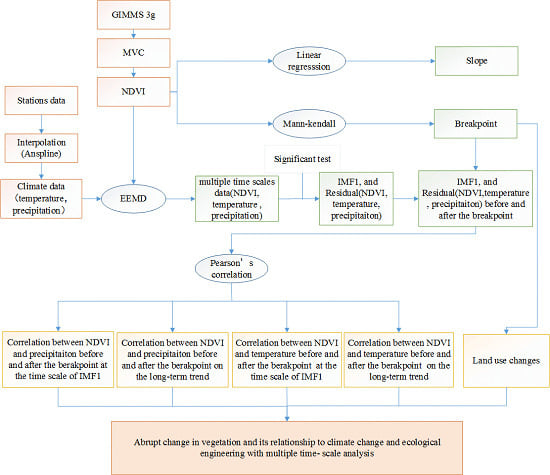
2. Materials and Methods

2.1. Study Area

The southwestern karst region of China (97°26′E–112°03′E, 21°9′N–34°22′N) includes Guangxi Province, Yunnan Province, Guizhou Province, Sichuan Province, and Chongqing municipality (Figure 1), with an area of 470,000 km². This region experiences a subtropical and tropical monsoon climate and the areas border the Tropic of Cancer, with a mean annual temperature of 20 °C and precipitation of 1450 mm [15]. The karst area in this region is approximately 63.5%, which is vulnerable to soil erosion and threatened by rock desertification [48]. Vegetation in Karst area is easy to be destroy, but hard to restore. The terrain of the study area is dominated by mountains, and the elevation decreases from the southeast to the northwest, ranging in a large scope. Due to the widely distributed mountains, there are differences in temperature, precipitation, vegetation types, and elevation in this karst region. The current land use types of this region are croplands, and mixed forests that have resulted from long-term anthropogenic activity and a highly dense population [51]. These natural and social characteristics of this region are the possible provide a unique terrestrial ecosystem for studying how vegetation dynamics respond to climate change and human activities.

2.2. Data Sources

The normalized difference vegetation index (NDVI) as an indicator of the vegetation greenness, has proven to be particularly useful for monitoring and characterizing the response of vegetation across a wide range of time periods, from abrupt natural events to seasonal variability of plant phenology caused by changes in temperature and abundant rainfall [52]. In this study, AVHRR NDVI3g, from the Global Inventory Modeling and Mapping Studies, was selected to monitor long-term trends in vegetation activity. The NDVI3g time series is an improved 8-km normalized difference vegetation index (NDVI) data set produced from the Advanced Very High Resolution Radiometer, which is provided by the Ecological Forecasting Lab at NASA Ames Research Center [53]. The dataset is a global composite product that spans from July 1981 to December 2015 with a spatial resolution of 1/12° and a bi-weekly interval [54]. It has been corrected for orbital drift, sensor calibration, viewing geometry, volcanic aerosols, atmospheric water vapor and cloud cover, and other errors unrelated to vegetation change [55]. NDVI has negative values in the place covered by cloud, water and snow, and thus will be affected by the atmosphere (cloud, water-vapour, and aerosols). To minimize the influence of the atmosphere and of the viewing and illumination conditions, the maximum value composite (MVC) technique was developed by Holben (1986), which has been widely used in many previous studies to deal with the NDVI3g data [56,57,58,59]. In this study, MVC was used to aggregate the original biweekly NDVI series into monthly series. In MATLAB, the moving averaged filter analysis was used to eliminate the abnormal values in time-series NDVI data [60,61]. To reflect the vegetation more appropriately, the NDVI products were averaged over an entire growing season from April to October to obtain the growing-season NDVI, which is usually used to represent the annual NDVI [62]. For each pixel, a mean growing-season NDVI <0.1 for the entire study period indicated barren and/or sparsely vegetated areas, which was excluded from the analysis to minimize soil background influences and enhance green vegetation signals. Previous studies have demonstrated that there was an overall acceptable agreement between GIMMS NDVI3g and multi-satellite NDVI products on regional to global scales [63].

Monthly rainfall and temperature datasets for the study area were collected from the Chinese meteorological data service from 1982–2015 [62]. There are 131 weather stations located in the study area. Based on the covariates of latitude, longitude and elevation (DEM), these data were interpolated to continuous surface data with an 8 km spatial resolution to match the NDVI dataset, using thin-plate smoothing spline model in ANUSPLIN4.4 [64,65]. The accuracy of the site values and interpolations were verified and finally passed the accuracy verification. Then, meteorological data were extracted by using MATLAB R2016b. They were then used for further analysis in ArcGIS. The growing-season (from April to October) summed precipitation and growing-season mean temperature were then calculated as two primary influencing climatic factors.

Land use data were collected from the Institute of Geographic Sciences and Natural Resources Research [10], which is based on US Landsat remote sensing image data, and obtained using through manual visual interpretation. In ArcGIS10.2, the data of the study area in 1980, 2000, and 2015 were obtained by pre-processing using commands such as clip, merge, intersect and reclassify. The forests and farmland in the land use type were extracted separately. Using the transfer matrix, the land use transfers from 1980 to 2015, before the abrupt change (1980–2000) and after the abrupt change (2000–2015) were obtained.

2.3. Mann-Kendall Abrupt Change Test

In this study, the Mann-Kendall nonparametric test was used to study the abrupt change in the growing season NDVI over the last 34 years in the karst region of southwest China.

For a time series, $X(t)=x_i,i=1,2,\cdots N$, where $x_i$ is the independent and identically distributed and $N$ is the number of data point. The statistic $S_k$ is defined as followed [66]:

$$S_k={\displaystyle \sum _{i=1}^k{r}_i,(k=2,3,\cdots ,n)}$$

(1)

with

$$r_i=\{\begin{array}{c}1,x_j-x_i>0\\ 0,x_j-x_i\le 0\end{array}\begin{array}{c}\\ ,\\ \end{array}(j=1,2,\cdots ,i)$$

(2)

In Equation (2) $x_i$ and $x_j$ are the ith data value in time series.

The trends can be determined using the standard normal test statistic, $U{F}_k$ calculated from Equation (3):

$$U{F}_k=\frac{[S_k-E(S_k)]}{{[Var(S_k)]}^{1/2}}, (k=2,3,4,\cdots n)$$

(3)

where UF₁ = 0. $E(S_k)$ and $Var(S_k)$ are the mean and variance of $S_k$, which can be calculated as follows:

$$E(S_k)=n(n-1)/4$$

(4)

$$Var(S_k)=n(n-1)(2n+5)/72$$

(5)

Positive (negative) values of $U{F}_k$ indicate increasing (decreasing) trends. A typical significance level of $\alpha =0.05$ was used in the test with $U{F}_{1-\alpha /2}$ = 1.96. If |$U{F}_k$| > 1.96, then, the null hypothesis of no trend is rejected, implying that there is a significant trend. For abrupt change point detection, another test statistic, $U{B}_k$ was introduced and calculated the same way as $U{F}_k$ by inverting the sequence of the time series $X_N,X_{N-1},\cdots X_1$. When the intersection point of the curves of $U{B}_k$ and $U{F}_k$ fell into the confidence interval, it indicated the time of an abrupt change. This method is not only simple to calculate the abrupt change point, but can also find out when and where the abrupt change starts, and it is widely used in vegetation, hydrology, and meteorology [67,68]. The Mann-Kendall abrupt change test was done in MATLAB R2016b.

2.4. Linear Regression Analysis

A linear regression analysis was conducted to analyze the monotonic trend of the NDVI. The trend slope in a multi-year regression equation represents inter-annual change, and can be solved using the ordinary least squares method (OLS), as follows:

$$Slope=\frac{n\times {\displaystyle \sum _{t=1}^{n}t\times NDV{I}_t-{\displaystyle \sum _{t=1}^{n}t{\displaystyle \sum _{t=1}^{n}NDV{I}_t}}}}{n\times {\displaystyle \sum _{t=1}^n{t}^2-{\left({\displaystyle \sum _{t=1}^{n}t}\right)}^2}}$$

(6)

where slope refers to the inter-annual trend in the growing-season NDVI; n is the number of years simulated; and the growing-season $NDV{I}_t$ is the value of this index in the tth year. A positive slope indicates vegetation greening, while a negative one indicates vegetation browning [4]. The significance of variation was determined using F-tests to calculate confidence levels (p < 0.05). Additionally, the change percentages of the NDVI in each case corresponded to the ratio between slope and the averaged NDVI. The slope analysis was done in MATLAB R2016b.

2.5. Ensemble Empirical Mode Decomposition (EEMD)

NDVI change is often nonlinear and nonstationary. It is a composition of a limited number of components with different frequencies due to noise, annual variations, inter-annual fluctuations, long-term trends, or even abrupt changes caused by disturbance events [69]. The inter-annual variation components of NDVI and climate changes are considered crucial for the understanding and prediction of the effects of an increasingly unstable climate on an ecosystem [70].

The EEMD method is based on empirical mode decomposition (EMD), which is also a noise assisted data analysis [44]. The EMD method can decompose time series data into a finite set of functions called intrinsic mode functions (IMFs) and a residual according to the local temporal and structural characteristics of the data. The decomposition process can be described as the following [71]:

Step 1. All of the local extrema of the original time-series X(t) ($t=1,2,\cdots ,N$, N is time length) need to be identified, and then all of the local maxima and minima need to be found using cubic spline interpolation to create the upper and lower envelopes. The first component $h_1(t)$ is calculated as the following:

$$h_1(t)=X(t)-d_1(t)$$

(7)

where $d_1(t)$ is the mean of the upper and lower envelopes.

Step 2. Since $h_1(t)$ is still not a stationary oscillatory pattern, the above process is repeated as:

$$h_{11}(t)=h_1(t)-d_{11}(t)$$

(8)

where $d_{11}(t)$ is the mean of the envelopes of $h_1(t)$. The second subscript index indicates the additional repetition number for the sifting process.

Step 3. When the following standard deviation (SD) is smaller than a pre-given value that is suggested to be set between 0.2–0.3 and is fixed as 0.2 in this case, the repeating process will stop.

$$SD={\displaystyle \sum _{t=1}^N\left[\frac{{\left|h_{1k}(t)-h_1{}_{(k-1)}(t)\right|}^2}{h^2{{}_1}_{(k-1)}(t)}\right]}$$

(9)

then

$$h_{1k}(t)=h_1{}_{(k-1)}(t)-d_{1k}(t)$$

(10)

where k is the number of iterations.

Therefore, the data derived in the first IMF component is (c₁ = h_1k(t)), and then the rest of the data is:

$$r_1=X(t)-c_1$$

(11)

Step 4. Since $r_1$ still contains oscillations of longer period, the process is repeated for all the subsequent $r_i$ described as:

$$r_i=r_{i-1}-c_i,i=2,3,\cdots n$$

(12)

$$X(t)={\displaystyle \sum _{i=1}^n{c}_i}+r_n$$

(13)

where n is the number of IMFs, $c_i$ is the ith IMF component, and $r_n$ is the residual. The sifting process will stop when the residual $r_n$ becomes a monotonic function or contains at most one extreme. Thus, a finite number of IMFs with decreasing frequency and a residual trend $r_n$ were extracted from the original time series according to the intrinsic characteristic of the sequence itself.

However, for EMD, there is a problem caused by mode mixing, which can result in an overestimation of the noise in the signal. Therefore, the ensemble EMD (EEMD) method was advanced by adding white noise to the original series as follows:

Step 5. Add a number $(l)$ of Gaussian white noise $p_j(t)$ to the original signal $x(t)$ to obtain a number of noisy pseudo signals $X_j(t)$.

$$X_j(t)=x(t)+p_j(t),j=1,2,\cdots l$$

(14)

$l$ is adopted as 1000 in this paper.

Step 6. Apply EMD method to these noisy pseudo signals $x_j(t)$.

Step 7. The ith EEMD IMFs $c_i(t)$ and $r_n$ are obtained by averaging the corresponding EMD IMFs and residual of these noisy pseudo signals as the following:

$$c_i(t)=\frac{1}{l}{\displaystyle \sum _{j=1}^l{c}_{ij}(t)}\mathrm{and}{r}_n(t)=\frac{1}{l}{\displaystyle \sum _{j=1}^l{r}_{nj}(t)}$$

(15)

where $c_{ij}(t)$ and $r_{nj}$ denotes the ith IMF and $r_n$ from $x_j(t)$.

Thus, EEMD produces a finite number of IMFs and a residual $r_n$. Each IMF component represents the oscillation of the original time series at a one-time scale. The residual reflects the long-term trend of the original sequence.

Step 8. Each of the resulting IMFs is considered a function having symmetric envelopes defined by the local maxima and minima, and also having the same number of zero-crossings and extrema. Based on this definition, we can determine the mean period of the function by counting the number of zero crossing of the function [15]. Quasi-period = (the time between the start and end of the zero crossing)/((number of zero crossings − 1)/2). Each IMF component is thought to be quasi-periodic changes at a certain timescale, which is caused by different driving forces at different time scales.

Step 9. To evaluate the importance of different time scale fluctuations (IMF), the variance contribution rate is estimated by the following:

$$V{c}_i=Var(c_i)/\left[{\displaystyle \sum _{i=1}^{n}Var(c_i)+Var(r_n)}\right]$$

(16)

and

$$V{r}_n=Var(r_n)/\left[{\displaystyle \sum _{i=1}^{n}Var(c_i)+Var(r_n)}\right]$$

(17)

where $V{c}_{\mathrm{i}}$ and $V{r}_n$ are the variance contributions of the ith IMF components and the residual, respectively; $Var(c_i)$ and $Var(r_n)$ are the variance of the ith IMF components and the residual ($r_n$).

A MATLAB EMD/EEMD package with above stoppage criterion and end treatment is provided by National Central University [72].

2.6. Correlation Analysis

On the 34-year time series, Pearson’s correlation was used to analyze the correlations between NDVI and temperature/precipitation at different time scales for each pixel. Pearson’s correlation was performed using the function of [r, p] = corr (X,Y) in MATLAB R2016b, where r and p represent the correlation coefficient matrix and the significance test result matrix, respectively, and X and Y are vegetation changes and climate change, respectively.

In this study, based on the Mann-Kendall test, the abrupt change of the growing-season NDVI were calculated. The linear regression analysis was used to calculate the spatial distribution trend of the growing season NDVI. Multiple time series of the growing season NDVI, temperature and precipitation were performed based on EEMD, and the correlations between vegetation and climate before and after abrupt changes at different time scales were calculated using Pearson’s correlation (Figure 2).

3. Results

3.1. Temporal and Spatial Changes in Vegetation and its Abrupt Change

Figure 3 shows the abrupt change of the area-averaged growing-season NDVI and its spatial distribution in the karst region of southwest China for the period from 1982 to 2015. There was an intersection in 2001 falling into the confidence interval (Figure 3a), and so it was thought to be an abrupt change according to Mann-Kendall abrupt change test. Before the breakpoint (2001), the NDVI showed an insignificant trend. After the breakpoint, the NDVI trend shifted from insignificantly to significantly increasing. As shown from Figure 3b, the growing-season NDVI value in 1982–2015 ranged from 0.43 to 0.88, indicating a large spatial heterogeneity. The NDVI gradually decreased from east to west.

Figure 4a–f shows the spatial distribution of NDVI trends based on a linear regression analysis (Slope) during the entire period, before and after the abrupt change. During the entire period, the trend decreased from the southeast to the northwest. Approximately 83.21% of the study area exhibited a greening trend (Slope >0); and approximately 24.59% was characterized by a greening trend over a time span of 0.002 year⁻¹. The significantly greening trends were primarily located in the eastern part of the study area (Figure 4d), and the insignificantly browning trends were mostly located in the western part. Before the abrupt change, NDVI showed an insignificant trend throughout most of the study area and the area percentage of the significant trend only accounted for 19.69 % (Figure 4e). Approximately 77.36% of the vegetated area displayed greening trends, of which only 1.86% exceeded 0.004 year⁻¹. Approximately 22.64% of the vegetated area displayed browning trends (Slope <0), of which only 2.5% was below −0.004 year⁻¹. After the abrupt change, the vegetation trend changed from insignificant to significant greening or browning (Figure 4f). Specifically, the greening of the NDVI changed from insignificant to significant in the east, as did the browning in the west. The area percentage of the significant trend in the NDVI increased from 19.69% to 49.37%, with most greening located in the eastern part. More specifically, 18.65% of the vegetated area was characterized by a greening trend over 0.004 year⁻¹, and approximately 30.75% of the vegetated area displayed browning trends, of which 15.93% were below −0.004 year⁻¹. Overall, the greening trend in the east and the browning trend in the west changed from insignificant to significant after the abrupt change.

3.2. Possible Relationships of the Abrupt Change in the NDVI with Climate Change During the Entire Time Period

The anomaly time series (the anomaly data = the raw data − the trend) of the NDVI, temperature and precipitation were used to reveal the correlation between NDVI and climate change from the entire time period. As shown in Figure 5, the correlation between the NDVI and temperature was positive in the eastern part and negative in the western part of the study area from 1982 to 2015. The correlation was significantly negative in the Yunnan Province. Before the abrupt change, the correlation between the NDVI and temperature was similar to that of 1982–2015, but the area percentage with significantly positive correlation increased to 12.42%, and area percentage with the significantly negative correlation reduced to 2.51%. After the abrupt change, the correlation changed from significantly positive to significantly negative in the east, and the area percentage with the significantly negative correlation increased from 2.51% to 26.48%, while the area percentage with the significantly positive correlation reduced from 12.42% to 2.57%. The correlation between the NDVI and precipitation was negative in the northeast, and positive in the southwest. Before the abrupt change, the correlation between the NDVI and precipitation was similar to that of 1982–2015, and the area percentage of the significant correlation increased to 14.55%. After the abrupt change, the correlation between the NDVI and precipitation changed from negative to positive in the east, and the percentage of the significantly positive and significantly negative correlation increased to 8.46% and 13.05%, respectively.

3.3. Possible Relationships of the Abrupt Change in the NDVI with Climate Changes Based on Multiple Timescales Analysis

To reveal the relationship between abrupt changes in the NDVI and climate change, a multiple time-scale analysis for the growing-season NDVI, temperature, and precipitation was performed based on the EEMD method at the pixel scale. Figure 6 indicates the temporal changes in the average growing-season NDVI, temperature, and precipitation at different time scales (IMF1–4) and residuals by averaging the values of all pixels. Similarly,

Table 1. Average quasi-periods and their variance contributions to NDVI, temperature and precipitation changes at different time scales (IMF1–IMF4) and residuals of all pixels in the karst region of southwest China.

Variables	Types	IMF1	IMF2	IMF3	IMF4	Residual
NDVI	Quasi-periods	2.5 *	5.8	11.2	25
	Variance contribution rate (%)	29.54	12.12	9.41	0.38	48.55
Temperature	Quasi-periods	2.7 *	5.5 *	11.1	17.2
	Variance contribution rate (%)	56.4	25.84	8.79	0.58	9.55
Precipitation	Quasi-periods	2.73 *	6.50	15.67 *	37
	Variance contribution rate (%)	52.21	14.23	28.87	1.42	3.9

* Passing the 95% significance test.

indicates the quasi- periods and their variance contributions of NDVI, temperature and precipitation at different time scales.

Figure 6a and Table 1 shows that the IMF1-IMF4 components at the 2.5, 5.8, 11.2 and 25-year time scales and their variance contribution rate in the growing-season NDVI changes in southwest China. Among them, the 2.5-year time scale had the greatest variance contribution, and only it passed the significance test. Therefore, other time scales were not considered for the following study. The variance contribution of the residual was 48.55%, which was greater than that of any IMF component. Moreover, the residual showed an increasing trend as shown in Figure 5a. Therefore, the vegetation dynamics in the karst region of southwest China was characterized by oscillations of 2.5-years and residual.

As shown from Figure 6b,c and Table 1, the growing-season temperature changes in southwest China had four oscillations at the 2.7, 5.5, 11.1 and 17.2-year time scales, among which, the 2.5-and 5.5-year passed the significance test. In addition, over the long-term trend, the average temperature showed a decreasing trend from 1982–1990, and a slowly increasing trend from 1990–2000, then it increased rapidly after 2000. Growing-season precipitation changes in southwest China experienced four oscillations of at the 2.73, 6.5, 15.67, and 37-year time scales, among which, 2.7– and 15.8 passed the significance test. Precipitation showed an upward trend in 2000 and then a downward trend.

To reveal the spatial heterogeneity of the NDVI, the multiple time scale analysis was performed at each pixel scale. As shown in Figure 7, for the 2.5-year time scale, the temperature had negative relationships with the NDVI from 1982 to 2015, especially in the western parts of the study area, and the area percentage of the significant correlation accounted for 22.65%. Prior to the abrupt change, the correlation between the NDVI and temperature was negative in the western parts and positive in the eastern parts. After the abrupt change, it changed from insignificantly negative to significantly negative in the west, and the area percentage of the significantly negative correlation increasing from 7.23 to 13.43%. In most parts of the study area, the precipitation had negative relationships with the NDVI from 1982 to 2015, and the area percentage of the significantly negative correlation accounted for 11.51%, primarily located in the southwest and north. Prior to the abrupt change, the precipitation had positive relationships with the NDVI in the middle of the study area, and the area percentage of the significantly positive correlation was 4.1%. After the abrupt change, the correlation between the NDVI and precipitation was similar to that of 1982–2015, and the area percentage of the negative correlation increased from 4.96% to 13.49%, which became more concentrated in the west. Thus, the correlation between the NDVI and precipitation changed from insignificantly to significantly positive in the west. Meanwhile, the correlation changed from positive to negative in the northeast.

As shown in Figure 8, on the long-term trend, in most parts of the study area, the correlation between the NDVI and temperature was significantly positive in 1982–2015, accounting for 56.66% and primarily located in the southwest and the northeast of the study area. Prior to the abrupt change, the correlation was significantly negative in the southeast of the study area, while significantly positive in other places. After the abrupt change, the correlation changed from significantly negative to significantly positive in the east, while it changed from significantly positive to significantly negative in the west. Moreover, the area percentage of the significantly positive correlation increased from 36.52% to 66.25%. Prior to the abrupt change, the correlation between the NDVI and precipitation was similar to that of 1982–2015. Moreover, the changes in the correlation were very small before and after abrupt change.

3.4. Possible Impacts of the Grain to Green Project (GGP) on the Abrupt Change in Vegetation

The ecological engineering Grain to Green Project (GGP) was launched in 1999 in Sichuan, 2000 in Guizhou and Chongqing, and 2001 in Guangxi and Yunnan respectively. These time periods coincided with an abrupt change in NDVI. Thus, the land use changes before and after the abrupt change were compared to explore whether it was the GGP that caused the changes of the abrupt change in vegetation and its relationships to climate change.

Since vegetation and the correlation between temperature and the NDVI showed large differences in the eastern and western portions of the study area, the study area was divided into two parts, the east (consisting of the eastern part of Yunnan and Sichuan, all of Guizhou, Chongqing and Guangxi) and the west (in the western part of Yunnan and Sichuan). As shown in

Table 2. Conversion of farmland and forest before and after the breakpoint in the entire area, the west area, and the east area (km²).

Region	Transfer Type	1982–2015	Before the Breakpoint	After the Breakpoint
Overall area	Farmland converted to forest	1952.66	736.39	1287.15
	Forest converted to farmland	1531.78	938.04	658.40
West area	Farmland converted to forest	493.52	365.93	140.41
	Forest converted to farmland	384.07	344.76	51.17
East area	Farmland converted to forest	1454.34	369	1143.32
	Forest converted to farmland	1144.45	591.11	490.02

, in the overall area, after the abrupt change, the area of farmland converted to forest increased from 736.39 to 1287.15 km², and the forest converted to farmland decreased from 938.04 to 658.40 km². In the west, after the abrupt change, the farmland converted to forest reduced from 635.93 to 140.41 km². It is because the project in the west was the Natural Forest Protection Plan causing less land use changes. However, in the east, after the abrupt change, the area of farmland converted to forest increased from 369 to 1143.32 km², and forest converted to farmland reduced from 591.11 to 490.02 km². So, more farmland was converted to forests in the east, which increased vegetation cover. Therefore, it is possible that the GGP lead to an abrupt change in vegetation from insignificantly greening to significantly greening in the east, while it is possible the rising temperature led to the abrupt change from insignificantly browning to significantly browning in the west.

4. Discussion

In this study, the Mann-Kendall test was used to detect abrupt change in vegetation in the karst region of southwest China over 34 years (1982 to 2015). It was found that the NDVI had an abrupt change in 2001. Although the NDVI3g may be affected by orbital drift, cloud and some noise in 2001, it could only produce some abnormal values without significantly affecting the overall trend [53,73]. However, in our study, after the abrupt change, the greening trend of the NDVI in the east and the browning trend in the west both changed from insignificant to significant. Previous studies revealed that vegetation had an overall significantly greening trend in the karst region of southwest China during the entire time period, but they ignored the abrupt changes [74,75]. Our study found that, although the area percentage of significance of vegetation changes did not change much by comparing the entire period and the period after the abrupt change, in reality, the distribution of vegetation greening and browning trend changed substantially before and after the abrupt change. Thus, the abrupt change analysis helped to correctly reveal the actual trend in vegetation changes, moreover, the hidden transformation in the trend, which will avoid the underestimation or overestimation of the potential risk of vegetation browning.

Previous studies have analyzed that the relationship of vegetation change to climate change in the karst region of southwest China from the entire period, but ignored the abrupt change [76,77]. In this study, the relationships of the abrupt change in the NDVI with climate change during the entire time, before the abrupt change and after the abrupt change period were revealed. The result show that, after the abrupt change, the correlation between the NDVI and temperature changed from insignificantly negative to significantly negative in the west, but from significantly negative to significantly positive in the east. The correlation between the NDVI and precipitation changed from significantly negative to significantly positive in the southeast. Then, combined with multiple time-scale analysis, abrupt change analysis, and correlation analysis, it is found that the relationship between vegetation and climate changes before and after the abrupt change on different time scales were different with the entire period.

At the 2.5-year time scale, after the abrupt change, the correlation between the NDVI and temperature changed from insignificantly negative to significantly negative in the west, but it did not change significantly in the east. The negative correlation between precipitation and NDVI became more significant. In the west, the vegetation types are dominated by the needle-leaf forests, which prefer a lower temperature [74]. The temperature had an increasing trend. Moreover, after the abrupt change, the temperature increased rapidly, and the short-term increase of temperature would lead to increased evaporation, which was not suitable to vegetation growth [23]. Therefore, the relationship between temperature and NDVI changed from insignificantly negative to significantly negative in the west. After the abrupt change, the precipitation had a downward trend. The karst area is dominated by soluble rocks and is easily eroded by groundwater and surface water, resulting in soil erosion. The reduction of precipitation after the abrupt change was beneficial to soil and water conservation. Thus, the negative correlation between precipitation and NDVI has become more significant. Therefore, at the short time-scale, to improve the greening trend of vegetation, more attention should be paid to the sudden rising temperature in the west.

In the long-term trend, after the abrupt change, the correlation between NDVI and temperature changed from significantly negative to significantly positive in the east, while from significantly positive to significantly negative in the west. However, there were few changes in the relationship between NDVI and precipitation. In the west, the majority of the vegetation types is needle-leaf forest. Before the abrupt change, an appropriate increase in temperature and abundant precipitation could promote the growth of vegetation on the long-term scale. However, after the abrupt change, the sudden increase in temperature exceeded the vegetation growth threshold and hindered the vegetation growth [23]. So, the correlation between NDVI and temperature changed from significantly positive to significantly negative in the west. At the same time, the project in the west was the Natural Forest Protection Plan, the land use change had no effect in this area, and the abrupt change might be caused by rising temperatures. In the east, the temperature was much higher than that in the west. Before the abrupt change, the higher temperature led to enhanced evaporation, which restricted the vegetation growth. So, the NDVI had a significantly negative relationship with temperature. After the abrupt change, the temperature continued to increase, which should be more detrimental to the growth of vegetation. However, the significant correlation between the NDVI and temperature changed from significantly negative to significantly positive. Therefore, the increase in vegetation might be caused by human activities instead of climate in the east. In the karst region of southwest China, the Grain to Green Project (GGP) was launched in 2000/2001, which is very close to the breakpoint of the NDVI. The GGP offers grain, cash and free seedlings as compensation for rural households to re-establish forests, shrub and/or grassland, which lead to a significant increase in vegetation cover [78]. In this study, it was found that GGP played an important role in the vegetation greening trend in the eastern part of the study area, where about 1143.32 km² in farmland was converted into forests, and the forest area had significantly increased. Therefore, the abrupt change in the vegetation greening trend and its correlation with temperature was caused by ecological protection projects in the eastern part of the study area. However, at the same time, it was found that the relationship between the NDVI and climate change on the long-term time scale was similar to that before the abrupt change, indicating that NDVI changes are affected by climate on long-term time scales, but the abrupt change in vegetation are affected by ecological engineering. To improve the greening trend of vegetation, ecological engineering should continue to be implemented in the future in the east, and more attention should be paid to the sudden rising temperature in the west.

Most studies have revealed that, in the karst regions of southwest China, the temperature variation had more significant impacts on vegetation dynamics than the precipitation variations, and the ecological engineering may increase the vegetation cover and reduce the ecosystem sensitivity to climate perturbations [54,79,80]. However, these studies analyzed the relationship of vegetation change to climate change and human activities using a single scale, ignoring the multiple time scale and the abrupt change. Therefore, it is very necessary to study the abrupt change in vegetation and its relationship to climate from multiple time scales. Our previous study concluded that climate played a major role in vegetation changes over the long term trend, but did not explore the changes of the relationship between climate and vegetation before and after the abrupt changes, and thus cannot explore the dominant timescale and the driving factors of the abrupt change [23]. However, for the abrupt change in this study, it is climate change that played a major role in the west, but, in the east, it is ecological engineering. The changes in the area percentage of significant correlation between climate change and vegetation change before and after the abrupt change on the long-term trend were more obvious than those changes at 2.5-year timescale, which indicated that the abrupt change of vegetation happened by the long-term trend. Thus, by integrating the abrupt change analysis and multiple timescale analysis, we can explore the role of climate changes and ecological engineering in abrupt change of vegetation and determine the major timescale at which it occurred.

5. Conclusions

Based on the non-parametric Mann-Kendall test and the empirical mode decomposition (EEMD) method, the spatial heterogeneity of the NDVI and the possible relationships between its abrupt changes with climate change and human activities in the karst region of southwest China during 1982–2015 were revealed at multiple time scales. Overall, the NDVI showed an increasing trend, but had an abrupt change in 2001. After the abrupt change, the greening trend in the east and the browning trend in the west both changed from insignificant to significant. Based on the EEMD analysis, at the 2.5-year time scale, after the abrupt change, the correlation between the NDVI and temperature changed from insignificantly negative to significantly negative in the west, which was primarily caused by climate change, especially rising temperatures. In the long-term trend, the correlation between the NDVI and temperature changed from significantly negative to significantly positive in the east, which was mainly caused by ecological protection projects. However, in the west, the causative factor for the abrupt change of the significant browning trend in vegetation and its correlation with temperature was primarily the rising temperatures. Meanwhile, the abrupt change primary occurred in the long-term trend. Thus, the integration of the abrupt change analysis and the multiple timescale analysis can serve to deepen our understanding of the driving mechanisms of abrupt changes in vegetation and enable us to better manage karst ecosystems and maintain their sustainability under environmental changes.

The maximum value compositing (MVC) algorithm was used to suppress atmospheric effects, but it may over-estimate NDVI value and cause high bias [58]. Averaging method may avoid overestimation but cannot minimize the influence of the atmosphere (cloud, water-vapour, aerosols). Therefore, further work is needed to combine those two methods to improve NDVI data.

References

1. Peng, J.; Li, Y.; Tian, L.; Liu, Y.; Wang, Y. Vegetation Dynamics and Associated Driving Forces in Eastern China during 1999–2008. Remote Sens. 2015, 7, 13641–13663. [Google Scholar] [CrossRef]
2. Wang, Z.; Zhang, Y.; Yang, Y.; Zhou, W.; Gang, C.; Zhang, Y.; Li, J.; An, R.; Wang, K.; Odeh, I. Quantitative assess the driving forces on the grassland degradation in the Qinghai–Tibet Plateau, in China. Ecol. Inform. 2016, 33, 32–44. [Google Scholar] [CrossRef]
3. Pan, N.; Feng, X.; Fu, B.; Wang, S.; Ji, F.; Pan, S. Increasing global vegetation browning hidden in overall vegetation greening: Insights from time-varying trends. Remote Sens. Environ. 2018, 214, 59–72. [Google Scholar] [CrossRef]
4. Li, L.; Zhang, Y.; Liu, L.; Wu, J.; Wang, Z.; Li, S.; Zhang, H.; Zu, J.; Ding, M.; Paudel, B. Comparison of the Vegetation Effect on ET Partitioning Based on Eddy Covariance Method at Five Different Sites of Northern China. Remote Sens. 2018, 10, 1755. [Google Scholar] [Green Version]
5. Lü, Y.; Zhang, L.; Feng, X.; Zeng, Y.; Fu, B.; Yao, X.; Li, J.; Wu, B. Recent ecological transitions in China: Greening, browning, and influential factors. Sci. Rep. 2015, 5, 8732. [Google Scholar] [CrossRef] [PubMed]
6. Jong, R.D.; Verbesselt, J.; Schaepman, M.E.; Bruin, S.D. Trend changes in global greening and browning: Contribution of short-term trends to longer-term change. Glob. Chang. Biol. 2012, 18, 642–655. [Google Scholar] [CrossRef]
7. Chen, B.; Guang, X.; Coops, N.; Ciais, P.; Innes, J.; Wang, G.; Myneni, R. Changes in vegetation photosynthetic activity trends across the Asia-Pacific region over the last three decades. Remote Sens. Environ. 2014, 144, 28–41. [Google Scholar] [CrossRef]
8. Phillips, P.C.; Moon, H.R. Linear Regression Limit Theory for Nonstationary Panel Data. Econometrica 1999, 67, 1057–1111. [Google Scholar] [CrossRef] [Green Version]
9. Abera, T.A.; Heiskanen, J.; Pellikka, P.; Maeda, E.E. Rainfall–vegetation interaction regulates temperature anomalies during extreme dry events in the Horn of Africa. Glob. Planet. Chang. 2018, 167, 35–45. [Google Scholar] [CrossRef]
10. Jing, W.; Wang, K.; Zhang, M.; Zhang, C. Impacts of climate change and human activities on vegetation cover in hilly southern China. Ecol. Eng. 2015, 81, 451–461. [Google Scholar]
11. Yi, S.; Long, J.; Wang, H. Vegetation Changes along the Qinghai-Tibet Plateau Engineering Corridor Since 2000 Induced by Climate Change and Human Activities. Remote Sens. 2018, 10, 95. [Google Scholar] [Green Version]
12. Wen, Z.; Wu, S.; Chen, J.; Lu, M. NDVI indicated long-term interannual changes in vegetation activities and their responses to climatic and anthropogenic factors in the Three Gorges Reservoir Region, China. Sci. Total Environ. 2017, 574, 947–959. [Google Scholar] [CrossRef] [PubMed]
13. Lloret, F.; Escudero, A.; Iriondo, J.M.; Martínez-Vilalta, J.; Valladares, F. Extreme climatic events and vegetation: The role of stabilizing processes. Glob. Chang. Biol. 2012, 18, 797–805. [Google Scholar] [CrossRef]
14. Li, B.; Zhang, L.; Yan, Q.; Xue, Y.J. Application of piecewise linear regression in the detection of vegetation greenness trends on the Tibetan Plateau. Int. J. Remote Sens. 2014, 35, 1526–1539. [Google Scholar] [CrossRef]
15. Liu, H.; Zhang, M.; Lin, Z. Relative importance of climate changes at different time scales on net primary productivity-a case study of the Karst area of northwest Guangxi, China. Environ. Monit. Assess. 2017, 189, 539. [Google Scholar] [CrossRef] [PubMed]
16. Du, J.; Shu, J.; Yin, J.; Yuan, X.; Jiaerheng, A.; Xiong, S.; He, P.; Liu, W. Analysis on spatio-temporal trends and drivers in vegetation growth during recent decades in Xinjiang, China. Int. J. Appl. Earth Obs. Geoinf. 2015, 38, 216–228. [Google Scholar] [CrossRef]
17. Li, S.; Verburg, P.H.; Lv, S.; Wu, J.; Li, X. Spatial analysis of the driving factors of grassland degradation under conditions of climate change and intensive use in Inner Mongolia, China. Reg. Environ. Chang. 2011, 12, 461–474. [Google Scholar] [CrossRef]
18. Chen, T.; Peng, L.; Liu, S.; Wang, Q. Spatio-temporal pattern of net primary productivity in Hengduan Mountains area, China: Impacts of climate change and human activities. Chin. Geogr. Sci. 2017, 27, 948–962. [Google Scholar] [CrossRef]
19. Piao, S.; Nan, H.; Huntingford, C.; Ciais, P.; Friedlingstein, P.; Sitch, S.; Peng, S.; Ahlstrom, A.; Canadell, J.G.; Cong, N.; et al. Evidence for a weakening relationship between interannual temperature variability and northern vegetation activity. Nat. Commun. 2014, 5, 5018. [Google Scholar] [CrossRef] [Green Version]
20. Wei, F.; Wang, S.; Fu, B.; Pan, N.; Feng, X.; Zhao, W.; Wang, C. Vegetation dynamic trends and the main drivers detected using the ensemble empirical mode decomposition method in East Africa. Land. Degrad. Dev. 2018, 29, 2542–2553. [Google Scholar] [CrossRef]
21. Liu, Z.; Li, C.; Zhou, P.; Chen, X. A probabilistic assessment of the likelihood of vegetation drought under varying climate conditions across China. Sci. Rep. 2016, 6, 35105. [Google Scholar] [CrossRef] [PubMed] [Green Version]
22. Guan, B.T. Ensemble empirical mode decomposition for analyzing phenological responses to warming. Agric. For. Meteorol. 2014, 194, 1–7. [Google Scholar] [CrossRef]
23. Liu, H.; Zhang, M.; Lin, Z.; Xu, X. Spatial heterogeneity of the relationship between vegetation dynamics and climate change and their driving forces at multiple time scales in Southwest China. Agric. For. Meteorol. 2018, 256–257, 10–21. [Google Scholar] [CrossRef]
24. Hawinkel, P.; Swinnen, E.; Lhermitte, S.; Verbist, B.; Van Orshoven, J.; Muys, B. A time series processing tool to extract climate-driven interannual vegetation dynamics using Ensemble Empirical Mode Decomposition (EEMD). Remote Sens. Environ. 2015, 169, 375–389. [Google Scholar] [CrossRef] [Green Version]
25. Yin, Y.; Tang, Q.; Wang, L.; Liu, X. Risk and contributing factors of ecosystem shifts over naturally vegetated land under climate change in China. Sci. Rep. 2016, 6, 20905. [Google Scholar] [CrossRef] [PubMed] [Green Version]
26. Jiang, L.; Jiapaer, G.; Bao, A.; Guo, H.; Ndayisaba, F. Vegetation dynamics and responses to climate change and human activities in Central Asia. Sci. Total Environ. 2017, 599–600, 967–980. [Google Scholar] [CrossRef]
27. Hua, W.; Chen, H.; Zhou, L.; Xie, Z.; Qin, M.; Li, X.; Ma, H.; Huang, Q.; Sun, S. Observational Quantification of Climatic and Human Influences on Vegetation Greening in China. Remote Sens. 2017, 9, 425. [Google Scholar] [CrossRef]
28. Rui, L.; Xiao, L.; Zhe, L.; Dai, J. Quantifying the relative impacts of climate and human activities on vegetation changes at the regional scale. Ecol. Indic. 2018, 93, 91–99. [Google Scholar]
29. Yin, Y.; Ma, D.; Wu, S.; Dai, E.; Zhu, Z.; Myneni, R.B. Nonlinear variations of forest leaf area index over China during 1982–2010 based on EEMD method. Int. J. Biometeorol. 2017, 61, 977–988. [Google Scholar] [CrossRef]
30. Verbesselt, J.; Hyndman, R.; Zeileis, A.; Culvenor, D. Phenological change detection while accounting for abrupt and gradual trends in satellite image time series. Remote Sens. Environ. 2010, 114, 2970–2980. [Google Scholar] [CrossRef] [Green Version]
31. Wong, C.M.; Daniels, L.D. Novel forest decline triggered by multiple interactions among climate, an introduced pathogen and bark beetles. Glob. Chang. Biol. 2017, 23, 1926–1941. [Google Scholar] [CrossRef] [PubMed]
32. Wang, X.; Piao, S.; Ciais, P.; Li, J.; Friedlingstein, P.; Koven, C.; Chen, A. Spring temperature change and its implication in the change of vegetation growth in North America from 1982 to 2006. Proc. Natl. Acad. Sci. USA 2011, 108, 1240–1245. [Google Scholar] [CrossRef] [PubMed] [Green Version]
33. Wang, X.; Piao, S.; Xu, X.; Ciais, P.; MacBean, N.; Myneni, R.B.; Li, L. Has the advancing onset of spring vegetation green-up slowed down or changed abruptly over the last three decades? Glob. Ecol. Biogeogr. 2015, 24, 621–631. [Google Scholar] [CrossRef]
34. Zhao, F.; Xu, Z.; Huang, J. Long-Term Trend and Abrupt Change for Major Climate Variables in the Upper Yellow River Basin. J. Meteorol. Res. 2007, 21, 204–214. [Google Scholar]
35. Yang, Y.; Tian, F. Abrupt change of runoff and its major driving factors in Haihe River Catchment, China. J. Hydrol. 2009, 374, 373–383. [Google Scholar] [CrossRef]
36. Mann, H.B. Nonparametric test against trend. Econometrica 1945, 13, 245–259. [Google Scholar] [CrossRef]
37. Kendall, M.G. Rank correlation methods. Br. J. Psychol. 1990, 25, 86–91. [Google Scholar] [CrossRef]
38. Hamed, K.H. Trend detection in hydrologic data: The Mann–Kendall trend test under the scaling hypothesis. J. Hydrol. 2008, 349, 350–363. [Google Scholar] [CrossRef]
39. Panda, D.K.; Kumar, A.; Mohanty, S. Recent trends in sediment load of the tropical (Peninsular) river basins of India. Glob. Planet. Chang. 2011, 75, 108–118. [Google Scholar] [CrossRef]
40. Yue, S.; Wang, C.Y. The Mann-Kendall Test Modified by Effective Sample Size to Detect Trend in Serially Correlated Hydrological Series. Water. Resour. Manag. 2004, 18, 201–218. [Google Scholar] [CrossRef]
41. Meng, M. Study on the Influence of Abrupt Climate Variation on the Vegetation Based on NDVI. Meteorol. Environ. Res. Lett. 2011, 2, 68–71. [Google Scholar]
42. Jiang, H.; Li, C.; Li, H. An improved EEMD with multiwavelet packet for rotating machinery multi-fault diagnosis. Mech. Syst. Signal Process. 2013, 36, 225–239. [Google Scholar] [CrossRef]
43. Tong, W.; Zhang, M.; Yu, Q.; Zhang, H. Comparing the applications of EMD and EEMD on time–frequency analysis of seismic signal. J. Appl. Geophys. 2012, 83, 29–34. [Google Scholar]
44. Huang, N.E.; Shen, Z.; Long, S.R.; Wu, M.C.; Shih, H.H.; Zheng, Q.; Yen, N.C.; Chi, C.T.; Liu, H.H. The Empirical Mode Decomposition and the Hilbert Spectrum for Nonlinear and Non-Stationary Time Series Analysis. Proc. Math. Phys. Eng. Sci. 1998, 454, 903–995. [Google Scholar] [CrossRef]
45. Kong, Y.; Meng, Y.; Li, W.; Yue, A.; Yuan, Y. Satellite Image Time Series Decomposition Based on EEMD. Remote Sens. 2015, 7, 15583–15604. [Google Scholar] [CrossRef] [Green Version]
46. Han, S.L. Estimation of extreme sea levels along the Bangladesh coast due to storm surge and sea level rise using EEMD and EVA. J. Geophys. Res. Ocean. 2013, 118, 4273–4285. [Google Scholar]
47. Wang, D.; Shen, Y.; Li, Y.; Huang, J. Rock Outcrops Redistribute Organic Carbon and Nutrients to Nearby Soil Patches in Three Karst Ecosystems in SW China. PLoS ONE 2016, 11, e0160773. [Google Scholar] [CrossRef]
48. Wang, S.J.; Liu, Q.M.; Zhang, D.F. Karst rocky desertification in southwestern China: Geomorphology, landuse, impact and rehabilitation. Land. Degrad. Dev. 2004, 15, 115–121. [Google Scholar] [CrossRef]
49. Yang, J.; Wang, W.; Hu, M.; Mao, R. Extreme drought event of 2009/2010 over southwestern China. Meteorol. Atmos. Phys. 2012, 115, 173–184. [Google Scholar] [CrossRef]
50. Xiong, H.F.; Wang, S.J.; Rong, L.; Cheng, A.Y.; Li, Y.B. Effects of extreme drought on plant species in Karst area of Guizhou Province, Southwest China. Chin. J. Appl. Ecol. 2011, 22, 1127–1134. [Google Scholar]
51. Zhang, T.; Li, J.; Pu, J.; Martin, J.B.; Khadka, M.B.; Wu, F.; Li, L.; Jiang, F.; Huang, S.; Yuan, D. River sequesters atmospheric carbon and limits the CO2 degassing in karst area, southwest China. Sci. Total Environ. 2017, 609, 92. [Google Scholar] [CrossRef] [PubMed]
52. Gascon, M.; Cirach, M.; Martínez, D.; Dadvand, P.; Valentín, A.; Plasència, A.; Nieuwenhuijsen, M.J. Normalized difference vegetation index (NDVI) as a marker of surrounding greenness in epidemiological studies: The case of Barcelona city. Urban For. Urban Green. 2016, 19, 88–94. [Google Scholar] [CrossRef]
53. Prevot, T.; Smith, N.M.; Palmer, E.; Callantine, T.J.; Lee, P.U.; Mercer, J.; Martin, L.; Brasil, C.; Cabrall, C. An Overview of Current Capabilities and Research Activities in the Airspace Operations Laboratory at NASA Ames Research Center. In Proceedings of the 14th AIAA Aviation Technology, Integration, and Operations Conference, Atlanta, GA, USA, 16–20 June 2014. [Google Scholar]
54. Tong, X.; Brandt, M.; Yue, Y.; Horion, S.; Wang, K.; Keersmaecker, W.D.; Feng, T.; Schurgers, G.; Xiao, X.; Luo, Y. Increased vegetation growth and carbon stock in China karst via ecological engineering. Nat. Sustain. 2018, 1, 44–50. [Google Scholar] [CrossRef]
55. Tao, Z.; Wang, H.; Liu, Y.; Xu, Y.; Dai, J. Phenological response of different vegetation types to temperature and precipitation variations in northern China during 1982–2012. Int. J. Remote Sens. 2017, 38, 3236–3252. [Google Scholar] [CrossRef]
56. Liu, C.; Melack, J.; Tian, Y.; Huang, H.; Jiang, J.; Fu, X.; Zhang, Z. Detecting Land Degradation in Eastern China Grasslands with Time Series Segmentation and Residual Trend analysis (TSS-RESTREND) and GIMMS NDVI3g Data. Remote Sens. 2019, 11, 1014. [Google Scholar] [CrossRef]
57. Tong, S.; Zhang, J.; Ha, S.; Lai, Q.; Ma, Q. Dynamics of Fractional Vegetation Coverage and Its Relationship with Climate and Human Activities in Inner Mongolia, China. Remote Sens. 2016, 8, 776. [Google Scholar] [CrossRef]
58. Militino, A.; Ugarte, M.; Pérez-Goya, U. Stochastic Spatio-Temporal Models for Analysing NDVI Distribution of GIMMS NDVI3g Images. Remote Sens. 2017, 9, 76. [Google Scholar] [CrossRef]
59. Holben, B.N. Characteristics of maximum-value composite images from temporal AVHRR data. Int. J. Remote Sens. 1986, 7, 1417–1434. [Google Scholar] [CrossRef]
60. Zhang, Z.; Song, X.; Chen, Y.; Wang, P.; Wei, X.; Tao, F. Dynamic variability of the heading-flowering stages of single rice in China based on field observations and NDVI estimations. Int. J. Biometeorol. 2015, 59, 643–655. [Google Scholar] [CrossRef]
61. Golestan, S.; Ramezani, M.; Guerrero, J.M.; Freijedo, F.D.; Monfared, M. Moving Average Filter Based Phase-Locked Loops: Performance Analysis and Design Guidelines. J. IEEE Trans. Power Electron. 2014, 29, 2750–2763. [Google Scholar] [CrossRef]
62. Guan, Q.; Yang, L.; Pan, N.; Lin, J.; Xu, C.; Wang, F.; Liu, Z. Greening and Browning of the Hexi Corridor in Northwest China: Spatial Patterns and Responses to Climatic Variability and Anthropogenic Drivers. Remote Sens. 2018, 10, 1270. [Google Scholar] [CrossRef]
63. Joshi, N.; Baumann, M.; Ehammer, A.; Fensholt, R.; Grogan, K.; Hostert, P.; Jepsen, M.; Kuemmerle, T.; Meyfroidt, P.; Mitchard, E. A Review of the Application of Optical and Radar Remote Sensing Data Fusion to Land Use Mapping and Monitoring. Remote Sens. 2016, 8, 70. [Google Scholar] [CrossRef]
64. Hijmans, R.J.; Cameron, S.E.; Parra, J.L.; Jones, P.G.; Jarvis, A.J. Very high resolution interpolated climate surfaces for global land areas. Int. J. Climatol. 2010, 25, 1965–1978. [Google Scholar] [CrossRef]
65. Daly, C. Guidelines for assessing the suitability of spatial climate data sets. Int. J. Clim. 2010, 26, 707–721. [Google Scholar] [CrossRef]
66. Chen, Z.; Chen, Y.; Li, W. Response of runoff to change of atmospheric 0 °C level height in summer in arid region of Northwest China. Sci. China Earth Sci. 2012, 55, 1533–1544. [Google Scholar] [CrossRef]
67. Yue, S.; Pilon, P.; Cavadias, G. Power of the Mann–Kendall and Spearman’s rho tests for detecting monotonic trends in hydrological series. J. Hydrol. 2002, 259, 254–271. [Google Scholar] [CrossRef]
68. Liu, H.; Xu, X.; Lin, Z.; Zhang, M.; Ying, M.; Huang, C.; Hao, Y. Climatic and human impacts on quasi-periodic and abrupt changes of sedimentation rate at multiple time scales in Lake Taihu, China. J. Hydrol. 2016, 543, 739–748. [Google Scholar] [CrossRef]
69. Verma, R.; Dutta, S. Vegetation Dynamics from Denoised NDVI Using Empirical Mode Decomposition. J. Indian Soc. Remote Sens. 2013, 41, 555–566. [Google Scholar] [CrossRef]
70. Zhang, X.; Wang, K.; Yue, Y.; Tong, X.; Liao, C.; Zhang, M.; Jiang, Y. Factors impacting on vegetation dynamics and spatial non-stationary relationships in karst regions of southwest China. Acta Ecol. Sin. 2017, 37, 4008–4018. [Google Scholar]
71. Wu, Z.; Huang, E. Ensemble Empirical Mode Decomposition: A Noise Assisted Data Analysis Method. Adv. Adapt. Data Anal. 2011, 1, 1–41. [Google Scholar] [CrossRef]
72. Ji, F.; Wu, Z.; Huang, J.; Chassignet, E.P. Evolution of land surface air temperature trend. Nat. Clim. Chang. 2014, 4, 462–466. [Google Scholar] [CrossRef]
73. Pinzon, J.; Tucker, C. A Non-Stationary 1981–2012 AVHRR NDVI3g Time Series. Remote Sens. 2014, 6, 6929–6960. [Google Scholar] [CrossRef]
74. Cai, H.; Yang, X.; Wang, K.; Xiao, L. Is Forest Restoration in the Southwest China Karst Promoted Mainly by Climate Change or Human-Induced Factors? Remote Sens. 2014, 6, 9895–9910. [Google Scholar] [CrossRef] [Green Version]
75. Hou, W.; Gao, J.; Wu, S.; Dai, E. Interannual Variations in Growing-Season NDVI and Its Correlation with Climate Variables in the Southwestern Karst Region of China. Remote Sens. 2015, 7, 11105–11124. [Google Scholar] [CrossRef] [Green Version]
76. Wang, J.; Meng, J.J.; Cai, Y.L. Assessing vegetation dynamics impacted by climate change in the southwestern karst region of China with AVHRR NDVI and AVHRR NPP time-series. Environ. Geol. 2008, 54, 1185–1195. [Google Scholar] [CrossRef]
77. Jian, T.; Xu, T.; Dong, J.; Yu, X.; Jiang, Y.; Zhang, Y.; Ke, H.; Zhu, J.; Dong, J.; Xu, Y. Elevation-dependent effects of climate change on vegetation greenness in the high mountains of southwest China during 1982–2013. Int. J. Clim. 2017, 59, 780–794. [Google Scholar]
78. Qi, X.; Wang, K.; Zhang, C. Effectiveness of ecological restoration projects in a karst region of southwest China assessed using vegetation succession mapping. Ecol. Eng. 2013, 54, 245–253. [Google Scholar] [CrossRef]
79. Tong, X.; Wang, K.; Brandt, M.; Yue, Y.; Liao, C.; Fensholt, R. Assessing Future Vegetation Trends and Restoration Prospects in the Karst Regions of Southwest China. Remote Sens. 2016, 8, 357. [Google Scholar] [CrossRef]
80. Tong, X.; Wang, K.; Yue, Y.; Brandt, M.; Liu, B.; Zhang, C.; Liao, C.; Fensholt, R. Quantifying the effectiveness of ecological restoration projects on long-term vegetation dynamics in the karst regions of Southwest China. Int. J. Appl. Earth Obs. Geoinf. 2017, 54, 105–113. [Google Scholar] [CrossRef]
Figure 1. Location of the study area; and the spatial distribution of temperature, precipitation, vegetation types, elevation, and meteorological stations in southwestern China.
Remotesensing 11 01564 g001
Figure 2. A workflow of the research method process.
Remotesensing 11 01564 g002
Figure 3. The breakpoint and the spatial distribution of growing-season NDVI in the karst region of southwest China; (a) the abrupt change of NDVI, (b) the spatial distribution of mean NDVI from 1982 to 2015.
Remotesensing 11 01564 g003
Figure 4. The linear change rate and the significance level of the trend in the growing season NDVI. (ac) show the linear change rate of the NDVI trend in the entire period, before the breakpoint and after the breakpoint. (df) show the significance level of the NDVI trend during the entire period, before the breakpoint and after the breakpoint. The insets show the frequency distribution of the corresponding values.
Remotesensing 11 01564 g004
Figure 5. Significant correlation between temperature and NDVI in 1982–2015 (a), before the breakpoint (b), after the breakpoint (c); correlation between precipitation and NDVI in 1982–2015 (d), before the breakpoint (e), after the breakpoint (f). The insets show the frequency distribution of corresponding values.
Remotesensing 11 01564 g005
Figure 6. EEMD decomposition for (a) Average temporal changes in the growing-season NDVI, (b) temperature, and (c) precipitation during 1982–2015 in the karst region of Southwest China. IMF1-IMF4 components and residual represent different time scales and long term trend, respectively.
Remotesensing 11 01564 g006aRemotesensing 11 01564 g006b
Figure 7. Significant correlation between climate changes and the NDVI at the 2.5-year time scale in the karst region of southwest China: (a) correlation between temperature and NDVI from 1982–2015, (b) before the breakpoint; (c) after the breakpoint; (d) significant correlation between precipitation and NDVI from 1982–2015, (e) before the breakpoint, (f) after the breakpoint; (r: correlation coefficient; p: significance level). The insets show the frequency distribution of the corresponding values.
Remotesensing 11 01564 g007
Figure 8. Significant correlation between climate changes and the NDVI over the long-term trend in the karst region of southwest China: (a) correlation between temperature and NDVI from 1982–2015, (b) before the breakpoint, (c) after the breakpoint; (d) significant correlation between precipitation and NDVI from 1982–2015, (e) before the breakpoint, (f) after the breakpoint; (r: correlation coefficient; p: significance level). The insets show the frequency distribution of the corresponding values.
Remotesensing 11 01564 g008