Abstract
The temporal and spatial variability of the Antarctic coastline is a clear indicator of change in extent and mass balance of ice sheets and shelves. In this study, the Canny edge detector was utilized to automatically extract high-resolution information of the Antarctic coastline for 2005, 2010, and 2017, based on optical and microwave satellite data. In order to improve the accuracy of the extracted coastlines, we developed the Canny algorithm by automatically calculating the local low and high thresholds via the intensity histogram of each image to derive thresholds to distinguish ice sheet from water. A visual comparison between extracted coastlines and mosaics from remote sensing images shows good agreement. In addition, comparing manually extracted coastline, based on prior knowledge, the accuracy of planimetric position of automated extraction is better than two pixels of Landsat images (30 m resolution). Our study shows that the percentage of deviation (<100 m) between automatically and manually extracted coastlines in nine areas around the Antarctica is 92.32%, and the mean deviation is 38.15 m. Our results reveal that the length of coastline around Antarctica increased from 35,114 km in 2005 to 35,281 km in 2010, and again to 35,672 km in 2017. Meanwhile, the total area of the Antarctica varied slightly from 1.3618 × 10⁷ km2 (2005) to 1.3537 × 10⁷ km2 (2010) and 1.3657 × 10⁷ km2 (2017). We have found that the decline of the Antarctic area between 2005 and 2010 is related to the breakup of some individual ice shelves, mainly in the Antarctic Peninsula and off East Antarctica. We present a detailed analysis of the temporal and spatial change of coastline and area change for the six ice shelves that exhibited the largest change in the last decade. The largest area change (a loss of 4836 km2) occurred at the Wilkins Ice Shelf between 2005 and 2010.
1. Introduction
Knowledge of the coastline location forms the basis for coastal assessments and characterization of the land-ocean transition zone, and provides information on continental and coastal area [1]. The Antarctic coast is characterized by numerous ice shelves, which are permanent floating extensions of the glacial ice sheet onto the ocean. These ice shelves play an important role for ice sheet dynamics and mass balance. The Antarctic coastline region has a relatively high surface elevation, it is subjected to ~25% of the net ice sheet precipitation and covers 11% of Antarctica’s area. Defining the Antarctic coastline becomes crucial for assessment of the overall glacial mass budget and, particularly, ice sheet mass balance [2]. In this paper, the coastline of the Antarctica is defined as the boundary between the ocean and the ice sheet, which includes ice shelves. The coastal zones of Antarctica are affected by ongoing natural processes, such as iceberg calving (i.e., change in shape) and thinning (i.e., loss of ice shelf volume). Hence, coastline monitoring is of great importance to assess changes in the coastline configuration and ice sheet mass balance.
Recently, satellite remote sensing observations have offered an efficient means for mapping the continent of Antarctica [3], and have significantly improved the precision of coastline extraction. They have obviated the logistical obstacles of surface travel to obtain in situ data and the use of subjective manual delineation methods to map the coastline.
Typically, due to the contrast of albedo between the ocean and the snow-covered ice sheets, optical images are considered the most efficient data set to precisely delineate the coastline. They are also used for this purpose due to ease of accessibility and their extensive temporal record [4]. Different methods for delineating coastlines based on optical images have been proposed in the past few decades. An approach for automatic coastline detection based on snakes (parametric active contours) has been applied to Landsat images of Antarctica [5]. A new approach combining histogram thresholding and band ratio has been applied to extract the Urmia Lake coastlines from Landsat-7 Enhanced Thematic Mapper Plus (ETM+) and Thematic Mapper (TM) images [6]. Based on morphological tools, a new approach comprising two steps has shown promising results [7]. A spectral linear mixing approach (SLMA) has been utilized to assess coastline changes in southeastern Brazil based on TM and ETM+ images [8]. Although optical imagery is capable of generating high-resolution continuous coastlines with pixel-level precision, it is not suitable for polar regions since they are severely affected by cloud cover, seasonally reduced solar illumination, and other meteorological conditions [9]. Therefore, in order to improve the accuracy and continuity of the delineated coastline when Landsat images are affected by clouds, radar remote sensing data from synthetic aperture radar (SAR) have been used in this study.
With its ability to penetrate through clouds and its independence of daylight, SAR data have been used in a wide range of applications in the polar regions. A new automatic algorithm, based on pulse-coupled neural networks (PCNN), has been used to delineate coastlines by processing COSMO-SkyMed SAR products generated from different polarizations, geometric configurations, and measurement modes [10]. A novel algorithm (the modified K-means method and an adaptive coarse–fine object-based region-merging, MLAORM) for coastline extraction has been proposed for wide-swath Sentinel-1A images, which combines the modified K-means method and an adaptive coarse–fine object-based region-merging scheme [11]. More than 93% of the detected coastlines in Indonesia is located within 2-pixels distance in comparison with the manually traced coastlines [11]. Another new metric used to process dual-polarization coherent and incoherent SAR data for coastline extraction purposes allowed discriminating land from sea using an unsupervised classification scheme [12]. However, there are challenges in interpretation and analysis of SAR images due to the inherent speckle noise and possible overlap of backscatter from water and adjacent ice or land.
Previous coastline data sets of the Antarctica are available. A high-resolution Circum-Antarctic coastline has been derived from Radarsat-1 images collected during 1997 using a sequence of automated image processing algorithms [3]. A digital image mosaic of surface morphology of the Antarctic continent, assembled from 260 MODIS images, was generated. This data set was then used to determine the coastline vector files [13]. There are also some existing Antarctic coastline products, such as the Mosaic of Antarctica (MOA) coastlines (https://nsidc.org/data/moa) and Antarctica Digital Database (ADD) coastline (British Antarctic Survey, BAS; https://www.scar.org/data-products/Antarctica-digital-database/). Based on these data sets, we conducted a comprehensive analysis of the dynamic change of ice sheets at a finer spatial scale than previously. However, there are also some issues with these data sets. For one, the resolution of the MOA coastline product is 125 m and the resolution of our products is 30-75 m, which could provide a better analysis on the change of coastline as well as ice shelves. Traditionally, the coastlines are delineated by experts using optical images at a range of resolutions. Our automated method improves coastline extraction efficiency by removing biases associated with the subjective assessment.
In this study, we present detailed information of the Antarctic coastlines using high-resolution remote sensing data for three years: 2005, 2010, and 2017. The data were obtained from Landsat, Advanced Synthetic Aperture Radar (ASAR) on ENVISAT and SAR onboard Sentinel-1A/B (S1A/B). We modified the Canny edge algorithm [14] to improve the automated identification of the coastline.
2. Data
In order to generate coastline extraction results with higher resolution, Landsat and SAR images were used to identify the boundary between land (including glacier terminals and ice shelves) and open water. The quality of the image sources remains an important factor for coastline extraction, since optical sensors cannot be used during the period of polar nights [15]. This required us to focus on satellite-derived optical data for the austral summer (January to early March).
Landsat-7 Enhanced Thematic Mapper Plus (ETM+) images and Landsat-8 Operational Land Imager (OLI) images were used in this study. The data were downloaded in Geo-tiff format from the U.S. Geological Survey (USGS) website (USGS; https://www.usgs.gov/). The spatial resolution was 30 m for bands 1, 2, 3 of Landsat-7 and bands 2, 3, 4 of Landsat-8. The spectral bands of the OLI sensor provided a significant enhancement over the corresponding bands when compared to earlier Landsat instruments. For this study we selected scenes with less than 20% cloud cover. The current algorithm was applied to band 1 (Landsat-7) and band 2 (Landsat-8) data to identify the coastline. Color composite images (R, G, B) were also generated from Landsat-7 (bands 1, 2, and 3) and Landsat-8 OLI (bands 2, 3, and 4). These images clearly show the boundary between water and ice, and therefore, they were used to validate the output coastline as explained in Section 4.2.
Data from two SAR systems, onboard the Environmental Satellite (ENVISAT) and Sentinel-1 (both launched by the European Space Agency—ESA), were used in this study when atmospheric haze or cloud cover hindered the use of Landsat data (i.e., to fill gaps of Landsat-7 data under cloudy conditions). The Advanced SAR (ASAR) onboard Environmental Satellite (ENVISAT) operates in the C-band wavelength (5.3 cm) in different modes. This satellite was launched in 2002 and ceased operation in April 2012. We used the Wide Swath Mode (WSM) images at medium resolution (75 m) and a swath width of 400 km. Sentinel-1A and 1B are two satellites in a constellation, launched by ESA in April 2014 and 2016, respectively, carrying another C-band SAR. The data mode used in this study was the Interferometric Wide Swath (IW) with spatial resolution of 5 × 20 m. In our study, the polarization of both SAR systems was HH-polarization (horizontal transmit and horizontal receive). As for co-polarizations, HH-polarization is preferred for operational coastline delineation, because the clutter of ocean is more suppressed at HH-polarization than at VV-polarization (vertical transmit and vertical receive). Hence, imagery of the former is less noisy, and well suited for coastline extraction [16]. ASAR and Sentinel-1 data can be freely downloaded from the European Space Agency (ESA) website (https://www.esa.int/ESA). Table 1 presents information about the four sensors used in the study.

Table 1.
Characteristics of the Optical and synthetic aperture radar (SAR) images.
3. Method
There are three criteria that should be satisfied by any edge detector: Low error rate, good localization, and a single response to the edge [12]. Edge detections by different algorithms including Canny, LoG (Laplacian of Gaussian), Sobel, Prewitt, and Roberts have been compared, and the results obtained from the Canny algorithm were found to be most suitable under almost all scenarios [17,18]. Algorithms such as LoG, Sobel, Prewitt, and Roberts are sensitive to the noise. The increased noise in the images could eventually degrade the magnitude of the edges and the associated accuracy of its delineation. The Canny algorithm, on the other hand, improves the signal of edge points with respect to noise ratio by using non-maximum suppression, and provides better edge detection with the help of the threshold method [17,18]. The algorithm introduced in this study is an improvement to the Canny edge detector [13]. The three steps of the improved algorithm are: image preprocessing, automated edge detection method (with a modified element), and post-processing.
3.1. Data Pre-Processing
Here, Landsat-7/8 images were processed to L1GT (Systematic Terrain Correction) products, which provide the highest level of radiometric calibration and terrain correction (details can be found in the website of the United States Geological Survey-USGS, https://www.usgs.gov/). For Landsat-7 ETM+ and Landsat-8 OLI images, the terrain-corrected accuracy was 15 m and 12 m, respectively, in terms of 90% circular error (CE90, which means 90% of points have less than 15 m and 12 m positional error) [19,20]. On 31 May 2003, the Scan Line Corrector (SLC), which compensates for the forward motion of Landsat 7, failed. As a result, the imaged area became duplicated, with a width that increased towards the scene edge. We used ArcGIS de-striping tools to mitigate this effect. For Landsat-8 images, layer stacking and mosaic tools were utilized to generate the 2017 Antarctic coastline map. To improve the consistency of the extracted coastline, we had to ensure that there was sufficient overlap between neighboring images. As for SAR images, precise orbit files that contain accurate satellite position and velocity information have been employed to geocode the imagery, and the geometric accuracy of SAR (i.e., ASAR and Sentinel-1 SAR) data was less than 1 pixel [21,22]. Using SARscape software, backscatter calibration and range Doppler terrain corrections were applied. Backscatter calibration converted the Digital Number (DN) to a backscatter coefficient in decibels using calibration coefficients provided in image header files. Furthermore, the terrain correction shifted all the pixels to the correct geolocations according to the input DEM (digital elevation model) in the module of SARscape. The final extraction accuracy depends not only on the precision of improved Canny edge algorithm, but also on the geo-referencing accuracy of the Landsat and SAR images.
3.2. The Automated Edge Detection Method
Three sub-steps were required here: image smoothing, image gradient calculations and selection of threshold to identify edge pixels. The image smoothing step deals with bad strips commonly found in the Landsat-7 images and speckle noise common in radar data. Therefore, a smoothing filter was applied to suppress noise. Practical experiences have shown that the Gaussian filter can provide an acceptable compromise between noise immunity and accurate edge detection [23]. The larger the size of the kernel, the lower the detector’s sensitivity to noise. In order to maintain a good balance, we chose a kernel size of 5 and the standard deviation of 1.4.
In the image gradient calculations step, four filters were used to calculate image gradients along the horizontal, vertical, and the two diagonal directions, centered at each pixel in the image. This produced gradients in eight cardinal and ordinal directions at each pixel (0°, 45°, 90°, 135°, 180°, 225°, 270°, 315°). The gradient was calculated using the finite difference of the first-order partial derivative. The maximum of the eight gradients was selected to represent the edge strength, and the direction associated with this represented the direction perpendicular to the edge, which usually coincides with the highest gradient. The pixel was then identified as a possible edge pixel if the edge strength (gradient magnitude) was higher than a selected threshold. However, if we base the definition of the edge pixel on a single threshold of gradient values applied to all pixels, then the resulting edge may likely be blurred, noisy, and disconnected.
In the threshold selection step, to identify the potential edge pixel, we followed the Canny algorithm again but with a modification. In the original algorithm, two fixed global thresholds (high and low) on the gradient of the pixel value are manually set to filter out the false edges. If the gradient exceeds the high threshold, then the pixel is considered an edge pixel. If the gradient is less than the low threshold, then the pixel is not part of an edge and the DN will be set to zero. If the magnitude is between the high and low thresholds, then the pixel is considered as a “potential” edge pixel and the neighboring pixels are examined to confirm whether the edge is identified. If at least one pixel among the neighboring pixels exceeds the high threshold, then the pixel is identified as an edge pixel.
Based on experiments of extracting coastline with the original Canny algorithm, we found that the application of a fixed pair of thresholds to a sequence of spatially different images (around the Antarctica) yielded noisy images, as shown in Figure 1b. This is caused by the different contrast when the ice is subjected to surface deformation, metamorphosed snow cover, or when the water surface roughness varies due to varying surface wind field. Therefore, we introduced an adaptive threshold method to generate a pair of thresholds for each image. For each image, we examined the bimodality of the histogram of the pixel gradient and automatically identified the two clusters of edge and non-edge pixels with their different gradient magnitudes. This eventually led to improvement of the edge identification, as shown in Figure 1c.
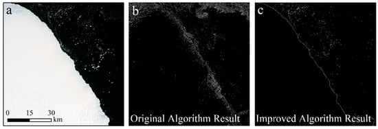
Figure 1.
Comparison between edge points from using a fixed pair threshold—for maximum and minimum (b), and an adaptive pair of thresholds (in the improved algorithm) (c). The corresponding Landsat-7 image shown in (a) was acquired on 25 January 2017. The improved edge detector yields much less noise and better continuity in the extracted coastline.
The selection of the adaptive thresholds (a pair representing the maximum and minimum associated with an image) is explained in Figure 2. For the three Landsat-8 images shown in panels a1a2, b1b2, and c1c2 (locations are marked in Figure 2d), the histograms of the gradients from all pixels of the images are presented in Figure 2e–g. All histograms feature tri-modal distribution (some feature bi-modal distribution but not shown). The two thresholds, which are selected automatically within the algorithm, are marked for each histogram. This is the added component to Canny’s method in this study. For each image, the high threshold is defined as the minimum of the highest-gradient cluster, and the low threshold is the maximum of the lowest-gradient cluster (Figure 2e). Based on this selection, the potential edge pixels are those having the gradient falling between the low and high thresholds (the blue area in each histogram). These pixels are examined to confirm their identity as being part of an edge or not using the same concept introduced in the Canny algorithm, as described above.
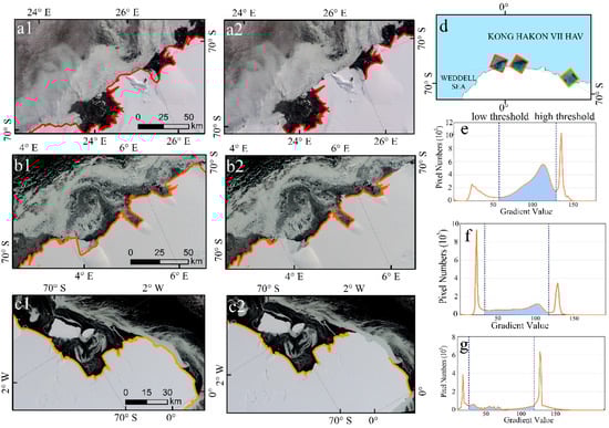
Figure 2.
Three pairs of Landsat-8 false color images (locations identified in (d)) are shown in (a1,a2), (b1,b2), and (c1,c2). Histograms of the pixel gradients are shown in (e–g), respectively. The two thresholds are marked by the blue-dashed lined in each histogram, while the blue gap between the two lines represents the gradient range for the potential edge points. Coastline extraction results using two thresholds and one threshold (the maximum threshold) are overlaid on the Landsat-8 images in the left and middle panels, respectively. The color composition we use is from bands 1, 2, and 3.
To check the revised Canny algorithm, we conducted two experiments to construct the edge. The first used the pair of high and low thresholds for each image, and the second used the maximum threshold only, and defined the edge pixels as those that have a gradient higher than that of the threshold. Results from the two experiments, after applying the complete method (including the post-processing step described in the next section), are presented in a1a2, b1b2, and c1c2 of Figure 2, respectively. It is clear that using a pair of adaptive thresholds (high and low) warrants the continuity of the edge (i.e., the coastline), which cannot be achieved using a single threshold when the edge is constructed from a sequence of spatial images.
3.3. Post-Processing Procedure and Edge Connection
Although we demonstrated the advantage of using an adaptive threshold over the use of a fixed value, Figure 2 reveals that the method still generates noisy edge pixels. Consequently, a median filter is used in the post-processing step to minimize the noise. The filter replaces the gradient at each identified edge pixel by the median of the gradients of the surrounding eight neighborhood pixels. This step proves to be efficient in reducing the spurious edge pixels. Finally, the precise geographical coordinates and projection information are automatically assigned to all edge pixels. This allows for edge segments extracted from different images around the Antarctic coast to be connected into one single polyline that can be further analyzed. To ensure consistency with the observed coastlines, the merged coastline is smoothed into the single polyline using the spatial analyst tool under ArcGIS environment.
4. Results and Analysis
4.1. Validation of Extracted Coastline
In order to assess the accuracy of the extracted coastline, we compared data from 2005 with 2004 MOA data. Figure 3 shows the comparison under the situation that the coastline is divided into five sectors: Weddell Sea (WS), Indian Ocean (IO), West Pacific (WP), Ross Sea (RS), and Bellingshausen Amundsen Seas (BAS). In general, the deviation between the two data sets is small (within a few kilometers). Insets in Figure 3 mark six areas of maximum deviation.
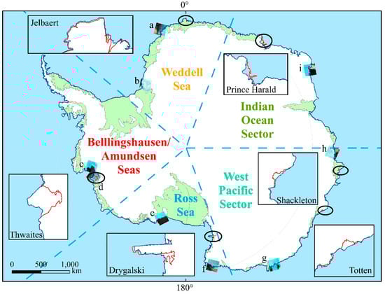
Figure 3.
Coastline from the present method (blue) compared to the 2004 Mosaic of Antarctica (MOA) coastline (red) for the entire Antarctic. The green color indicates the geolocations of ice shelves around the Antarctica. Samples from each sector that highlight areas of remarkable difference between the two data sets are shown in the insets. Also, marked by footprints of Landsat images are locations of nine areas (a–i) where statistical analysis of the difference between the automated and manually extracted coastline was performed. The zoomed in Landsat images of the nine areas are illustrated in Figure 4.
In this and the following section, we conducted a statistical analysis to characterize the deviation between our extracted coastlines and the validation coastline (in terms of the difference along the perpendicular line between the two data sets). Table 2 includes the number of occurrences, as well as statistical analysis of the deviation (measured in kilometers in the shown intervals), between the coastline from the present study in 2005 and the MOA-2004 data set for the given five sectors. In general, the deviation between the two data sets is small (within a few kilometers). The total number of pixel points in each sector varies between 1.7 × 10⁵ and 3.9 × 10⁵. Data were obtained from a sample of 10,000 points in each sector. Table 2 shows that the largest deviation is less than 5 km (indeed, there are many points with identical coastline between the two data sets). The average deviation is found to be maximum in the IO sector (1.81 km) and minimum in the RS sector (0.76 km). In the BAS sector, the deviation is also high (1.64 km), yet with maximum variability (St. Dev. 6.36 km). The maximum deviation of 66.37 km is also encountered in the sector. The deviation between the coastline from the present study and the MOA coastline (green line and yellow line in Figure 4) is relatively high, due to coarse resolution (125 m) in the latter and the interannual difference between two data sets, as well as the differences in the methods used to delineate coastlines.
Table 2.
Percentage of deviation between the coastline products from the present method in 2005 and the MOA 2004 data set for the five sectors (in km).
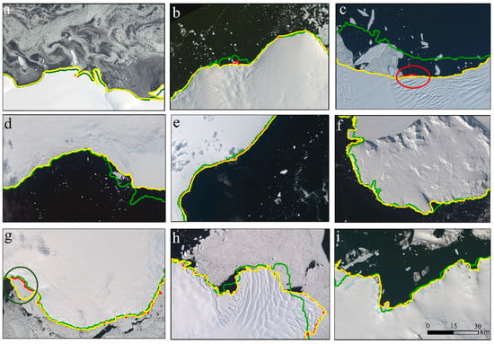
Figure 4.
Coastline in 2010, derived from present automated method (yellow) compared to the manually extracted coastline (red) from same image, and MOA coastline (green) in 2009 for the nine areas. The nine areas shown here are marked by footprints of Landsat images labeled as areas (a–i) in Figure 3.
The length of the Antarctic coastline calculated from MOA data in 2009 and the present data in 2010 for the five sectors are shown in Table 3. For the MOA in 2009, the total length of the Antarctic coastline is 39,608 km and the length of the coastline for each sector is 4750.71 km (WS), 13,868.27 km (BAS), 6776.71 km (RS), 6833.04 km (WP), and 7379.27 km (IO). Compared to the length for each sector from the present results in 2010, the length in 2009 is always greater except for the coastline in the WS. The mean difference of length in these five sectors is 865.32 km. The difference (2010–2009) in each sector is 165.46 km (WS), −1645.29 km (BAS), −971.72 km (RS), −989.75 km (WP), and −885.30 km (IO). The coastline in MOA was extracted manually and the contour is less smooth than the output from the present results.
Table 3.
Coastline length in each sector (km) in 2009 (MOA) and 2010 (this study). WS, Weddell Sea; BAS, Bellingshausen Amundsen Seas; RS, Ross Sea; WP, West Pacific; and IO, Indian Ocean.
4.2. Comparison Against Manual Extraction
The extracted coastlines in the nine areas from 2010 data, marked by the footprints of Landsat images in Figure 3, were compared to the manually extracted coastline based on visual interpretation of Landsat images. Results are presented in Figure 4 with the MOA-2009 coastline included. Visual comparison confirms a small deviation between the manual and automated extraction methods. However, in Figure 4c, there is a large discrepancy because the data for MOA coastline [24,25] are from a different year when compared to our data. This suggests a remarkable temporal change of the coastline in that area.
In addition, we chose 1000 points, at 60 m interval, in each area and computed their deviation from the manually extracted coastline. The visual comparison is shown in Figure 4 and the distribution of the deviation is included in Table 4. The range of deviation is divided into five bins, as shown in Table 4 (note that, unlike Table 2, units are in meters). The number of occurrences within each bin is also shown. Of the differences, 92.32% are within 100 m, with mean values between 19.47 m (Figure 4i) and 71.39 m (Figure 4g). The overall mean deviation is 38.15 m and the greatest deviation is 586.27 m, noticed in Figure 4c and the minimum deviation is 0 m.
Table 4.
Deviation between the coastline in 2010 from our method and the manually extracted coastline for the nine areas (in meters). Areas (a–i) are marked in Figure 3.
Based on examination of the data from this test, we found that errors over 100 m were mainly the results of the misinterpretation of offshore sea ice as being a part of an ice sheet (i.e., part of the continent), such as the part in the brown circle in Figure 4g. Additionally, these errors could have been caused by the manual extraction of coastline from a Landsat image when fast ice was misidentified as part of the ice sheet, such as the part in the red circle in Figure 4c.
4.3. Temporal Change of Coastline
Figure 5 shows the maps of the Antarctic coastline from 2005, 2010, and 2017 data with detailed information. Based on visual interpretation of maps in the five sectors, the most significant changes occurred in the BAS, while the WS experienced modest changes. The extracted coastlines were used to precisely calculate the total length of the coastline and area of the Antarctic continent using ArcGIS software environment in the Stereographic_South_Pole projected coordinate system. The length of each sector and the total length of the Antarctic coast are presented in Table 5. The rate of change of the total length from 2005 to 2010 was +33.4 km/year, and from 2010 to 2017 was +55.9 km/year. The rate of cumulative change from 2005 to 2017 was 46.5 km/year. In 2005, the area of the Antarctic was 1.3618 × 10⁷ km2 and it decreased to 1.3537 × 10⁷ km2 in 2010 at a rate of −16,137.46 km2/year. In 2017, the area increased to 1.3657 × 10⁷ km2, which is larger than the area of 2005. The rate of cumulative change from 2005 to 2017 is +1627.75 km2/year.
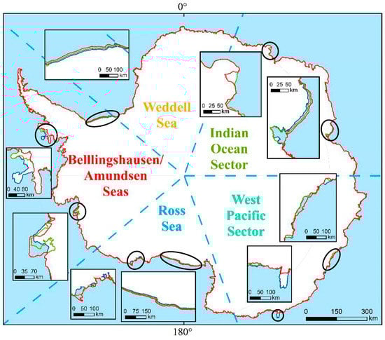
Figure 5.
Coastline contours from the present algorithm for 2005, 2010, and 2017 (blue, green, and red, respectively). The deviation between the contours is very small (<10 km) in most locations, but the insets highlight the nine areas with highest deviation between 2005 and 2017.
Table 5.
Change of coastline length in each sector (km) during 2005–2017.
As shown in Table 5, the length of the coastline reveals an overall increasing trend during 2005–2017, by 558.73 km in total. However, with some regional variability leading to the increase or decrease of length of the coastline in each sector, the largest change of length occurred in the BAS sector during 2005–2010 and the smallest occurred in the WS sector during 2010–2017. Only two sectors (WS and IO) showed a monotonic change of the length; increase in IO and decrease in WS. The other three sectors (BAS, RS, and WP) underwent increases and decreases. The East Antarctica encompasses the IO and WP sectors and the length of coastline in these two sectors increased to 6626.55 km and 6108.01 km in 2017, respectively. By analyzing the spatial change of ice shelves, we found that this increment is mainly due to the breakup of ice shelves (such as Amery Ice Shelf and Shackleton Ice Shelf) in these two sectors, which exposed more parts of ice sheet to the sea water and therefore increased the length of the outer border of the ice sheet. Detailed information is presented in Section 4.4.
In order to confirm the length change of coastline, we also calculated the differences between MOA in 2004 and 2009, as well as the differences between our extraction results in 2005 and 2010 (Table 6). From the MOA coastlines, the total length decreased by 284.90 km. However, the length of the coastline in the BAS and IO sectors increased while the length in the WS, RS, and WP sectors decreased between 2004 and 2009. On the other hand, based on our results (between 2005 and 2010), the direction of the change of length (increase/decrease) is the same in each sector as in the MOA data, though our results consistently exhibit less changes than the MOA data. The increase of 167.25 km in the total Antarctic coastline length from 2005 to 2010 in our results disagrees with a reduction of 284.90 km from 2004 to 2009 from the MOA data.
Table 6.
Deviation of coastline length in each sector (km) between MOA products (2004 and 2009) and our results (2005 and 2010).
4.4. Changes of Coastline in the Regions Around Six Ice Shelves
The area of Antarctica calculated from our 2005 results was 1.3618 × 10⁷ km2. Taking the temporal change (retreat and advance) of individual ice shelves around the Antarctica into consideration, the total Antarctic area underwent a decline from 2005 to 2010 at an average rate of 1.62 × 10⁴ km2/year. In 2010, the measured area was 1.3537 × 10⁷ km2. However, by 2017 there was an increase in total area to 1.3657 × 10⁷ km2 at an average rate of 1.71 × 10⁴ km2/year. As area change is mainly caused by the expansion or retreat of individual ice shelves, we investigated the evolution of six ice shelves. for each ice shelf, we calculated the largest area change and the highest rate of change. As shown in Figure 6, we monitored the area changes of Ronne Ice Shelf (RIS), Amery Ice Shelf (AIS), Mertz Glacier Tongue (MGT), Ross Ice Shelf (RSIS), Wilkins Ice Shelf (WIS), and Pine Island Shelf (PIS).
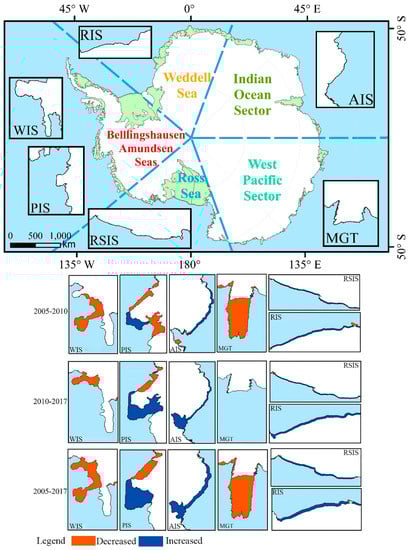
Figure 6.
Locations of six ice shelves along the Antarctic coast, which have undergone significant changes from 2005 to 2017. The green color indicates the geolocations of ice shelves around the Antarctica. The area changes of six ice shelves from 2005 to 2017 are shown below. The red shading indicates the area decreased and the blue shading indicates the area increased over this period. The contours are of the 2005 coastline from the present calculations. Data of 2005–2010 for MGT are up to end of March 2010 (i.e., after the calving of the giant iceberg C28). WIS, Wilkins Ice Shelf; PIS, Pine Island Shelf; AIS, Amery Ice Shelf; MGT, Mertz Glacier Tongue; RSIS, Ross Ice Shelf; and RIS, Ronne Ice Shelf.
In Figure 6, the shape and areal change of shape of the six ice shelves between 2005–2010, 2010–2017, and 2005–2017 have been depicted by two different colors: Blue for increase of area and red for decrease. Over the 12 years from 2005, there was dominant increasing trend in the AIS, PIS, RSIS, and RIS shelves (with minor decrease in some sections). Conversely, from 2005 to 2017, the area of the WIS and MGT shelves decreased.
The change of area of each ice shelf for each of the three periods is shown in Table 7. Area decline for individual ice shelves peaked between 2005 and 2010 at the WIS (4836 km2), while the least decline occurred between 2010 and 2017 at the MGT (67 km2). Conversely, the most significant increase of area for individual ice shelves happened in the RIS (3887 km2) during 2010–2017, and the smallest expansion happened in the AIS (698 km2) during 2005–2010.
Table 7.
Deviation of coastline area in each sector (km2) during three intervals.
Different ice shelves retreat at different rates, triggered by minor or significant collapse as well as the speed of ice flow. The rate of retreat is modulated by the ice shelf configuration and conditions of mass balance [26]. Based on the breakup time and the calved area, we give a detailed analysis of some decreasing ice shelves from 2005 to 2017.
One of the retreating ice shelves, the WIS, is located on the southwestern side of the Antarctic Peninsula. As shown in Table 6, it has been one of the fastest retreating ice shelves around Antarctica, especially from 2005 to 2010. It experienced a series of breakup events in 2008, revealing a number of different mechanisms for ice shelf disintegration [27]. In March 2008, it lost more than 400 km2 in a sudden collapse, and a further breakup of 160 km2 in the same area occurred in May during austral winter, as reported in [28]. In December 2008, new rifts developed, leading to a further breakup. As shown in Table 6, the area of WIS decreased by 4836 km2 from 2005 to 2010, and by a further 1900 km2 from 2010 to 2017. The ice shelf loss from 2005 to 2010 occurred at a much faster rate than that from 2010 to 2017. This is consistent with the series of breakup events in 2008, which accelerated the rate of loss. The total change rate is −561.33 km2/year. The large loss of area from the WIS supports a strong projection for a potential catastrophic loss of this ice shelf [28].
The MGT is a highly crevassed glacier in George V Land of East Antarctica. The ice velocity of the MGT typically exceeds 100 m/year [29]. The major calving event for the MGT occurred in February, 2010. An ice tongue about 78 km long and 36 km wide protruded 100 km out into the Southern Ocean, and broke away from the main body of the MGT to form a giant iceberg in February 2010 [30]. As shown in Figure 6, the coastline change between 2005 and 2010 captured this significant shape change. The length of the MGT decreased from 319.0 km in 2005 to 124.4 km in 2010, and then expanded slightly to 127.1 km in 2017. The area of the MGT decreased by 2582 km2 from 2005 to 2010, and by 2649 km² from 2005 to 2017. The total change rate is −220.75 km2/year. In another study, ASAR WSM data acquired on 9 January 2010 was used to extract the area of the disintegrated iceberg, which is estimated to be 2572 km2 [31]. This is in good agreement with the results presented here (2582 km2). The difference is likely due to the spatial resolution between the two data sets.
The PIS is a large ice stream, and the fastest changing glacier in the West Antarctica [32]. Therefore, its stability is of paramount importance to sea level rise and the mass balance of the West Antarctic Ice Sheet [33]. According to Table 6, its area decreased by 852 km2 from 2005 to 2010, then increased by 3174 km2 from 2010 to 2017. However, the loss pattern varies between different parts of the PIS, even for the same period. For example, from 2005 to 2010, there was expansion of PIS in some parts totaling 857 km2, and breakups in other parts with a total lost area of 1709 km2. This local response pattern across the PIS continued during the 2010–2017 period, with and expansion totaling 3490 km2 in some parts, and a loss of 516 km2 due to calving in other parts of the PIS.
Besides widespread local ice breakup events, some ice shelves have also undergone the reverse process (i.e., expansion), mainly in the more stable and wider East Antarctica ice sheet, such as the Amery Ice shelf. In the following, we calculate the expanded area and present an analysis of these expansion ice shelves.
The AIS is located at the head of the Prydz Bay in East Antarctica, with an area of approximately 60,000 km2 [34]. It is the third largest ice shelf in Antarctica, after the Ross Ice Shelf and the Filchner-Ronne Ice Shelf [35]. Between late 1963 and early 1964, a large piece of the ice shelf, about 9600 km2, calved and drifted to the west [36]. The calving front proceeded equator-ward from 2005 to 2017. In our results, there is a growing pattern shown in the area change, especially in the Prydz Bay. As shown in Table 6, the AIS increased by 698 km2 from 2005 to 2010 at a rate of +139.6 km2/year. It increased again by 2124 km2 from 2010 to 2017 at a rate of +303.4 km2 /year. The net rate is +235.2 km2/year.
The RSIS is the largest ice shelf in the Antarctica with an approximate area of 500,809 km2 in 2013 [37]. It is an important gateway through which signals of climate change approach West Antarctica. Based on coastline extraction results in this study, the coastline area increased by 2971 km2 from 2005 to 2010 at a rate of +594.2 km2/year, and increased by 3057 km2 from 2010 to 2017 at a rate of +436.7 km2/year. The net increase is 6028 km2 at a net rate of +502.3 km2/year. According to [31], between 2005 and 2017, observed sea-ice concentration increased and sea surface temperature (SST) decreased with maximum trends near the sea-ice margin (where ice expansion is likely to occur), in particular north of the RSIS.
The RIS is bounded on the west by the base of the Antarctic Peninsula. Although it has had several events of calving, the extracted coastlines still show a net expanding pattern from 2005 to 2017. In a previous study on the ice velocity changes in the Ronne Ice Shelf [38], it was concluded that the Ross and Filchner Ice Shelves exhibited signs of pre-calving events, representing the largest observed changes, with an increase in speed in excess of +100 m/year in 12 years. As shown in Table 6, the area increased by 2395 km2 from 2005 to 2010 at a rate of +479 km2/year. There is a much more obvious trend of coastline expansion from 2010 to 2017, when the area increased by 3887 km2 at a rate of +555.3 km2/year. The net rate is +523.5 km2/year.
Based on the area change of the RIS and the RSIS, we noticed that the expansion of ice sheet could impact on the shape of these shelves. These two shelves have advanced, but there is not much protrusion into the ocean. For the RIS and the RSIS, the longest linear distance between the corresponding points from the coastline in 2005 and in 2017 was 16.28 km and 14.17 km, respectively. On the other hand, we found that when the shelf protrudes deeply into the ocean it would likely become mechanically unstable, such as the calving of Larsen-B in 2002. When the ice shelf advanced into the ocean, oceanic factors (increased bottom melting and associated ice shelf thinning and recession) contributed to the structural weakness of the shelf, and consequently lead to the ice shelf breakup [39]. Another such example is MGT. From the result of the coastline in 2005, the shelf protruded into the ocean for more than 100 km, and in 2010 the unstable ice tongue broke into the ocean with the collision of the B-09 iceberg.
Among ice shelves with area expansion from 2005 to 2017, the area change, as well as the rate of the change, of the RIS and the RSIS were much more pronounced. Apart from these ice shelves with larger area change, there are also some other smaller ice shelves that underwent area and shape changes from 2005 to 2017. The Shackleton Ice Shelf, for example, enlarged by 1238 km2 from 2005 to 2010. The area of the Cook Ice Shelf decreased by 498 km2 from 2010 to 2017, while the area of the Lazarev Ice Shelf increased by 437 km2 over the same time.
5. Discussion
In this study, we applied a modified version of the Canny edge detection method to Landsat images in order to delineate the coastline of the Antarctica. The high resolution of the images was an essential factor for improvement in the precision of coastline products. Compared to existing coastline products from coarse-resolution MODIS data (Figure 4), Landsat-7/8 images reveal finer details and more accurate coastline results. The high deviation between the MOA coastline and our results in Table 2 is mainly caused by the data resolution, differences in acquisition dates, and the procedures of the extraction method. The manually delineated MOA-2004 coastline is derived from MODIS data acquired from November 2003 to February 2004, and the data we used were acquired from January 2005 to early March 2005. The resolution of MOA-2004 is 125 m and that of our result is 30–75 m.
We demonstrated the virtue of the improved coastline extraction algorithm, including its high resolution and the derived scientific and operational applications based on this method. By basing coastline mapping solely on remotely sensed data, the coastline extraction may be updated with little effort as more circum-Antarctic imagery becomes available.
While we sought to completely automate coastline extraction, there are a few instances when there is near-coastal fast ice attached to the glacial ice sheets or ice sheets shelves. Under these conditions, the edge of off-shore sea ice is automatically extracted as the coastline, and the uncertainty of coastline extraction using our method increases. Results in Table 4 show that the percentage of pixel points with deviation between the automatically and manually extracted coastlines >100 m is 17.5% and 21.3%, in Figure 4c,g. The corresponding percentage of deviation (>100 m) for the total 9000 points is 7.68%. The main cause of this deviation is that the automated processing cannot detect the differences in the gradient histograms between glacial ice and the adjacent fast ice. This consequently assigned the oceanic fast-ice area to the continental ice area, and the edge of fast ice was misjudged as the coastline. This issue is more crucial along the Antarctic Peninsula, where the intensity contrast between fast ice and ice shelves is weak. In this case, one has to rely on expert knowledge to post-process the extracted coastlines. Such misclassification errors may be corrected using the graphic editor tools within the ArcGIS software environment.
Therefore, further improvements, especially in the image-handling procedure, are recommended. For example, our processing algorithm requires a certain amount of compute time. Hence to maintain acceptable processing time, high-resolution optical images, such as the Landsat scenes, have to be split into sub-images for parallel processing. This could possibly impact the coastline displacement. Also, the spring tide, derived by data assimilation in the Filchner Ronne and Larsen Ice Shelves, could range 1–2 m and even exceed 3 m [40], but the impact on the horizontal movement of ice shelves with height exceeding over tens of meters is minor. Therefore, the tide may have virtually no influence on the location of coastlines. Also, for regions with low contrast, we intend to revise our algorithm by taking other data—such as ice velocity and in-situ observations—into consideration to yield higher extraction accuracy. Finally, we propose to combine a range of high-resolution imagery to feed into the automated algorithm with the aim to improve the accuracy of the extracted coastlines. This would include the integration of optical and radar data for improved interpretation of the spectral and structural coastline characteristics.
According to the fractal geometry theory, coastlines extracted from remote sensing images with different spatial resolution are discrepant [41]. The results from a previous study show that the spatial scaling of remote sensing data reduces the average error from 69.4 m to 58.3 m on the coastline with the length of 3871.3 m [42], which is minor. In our study, the impact of the difference in resolution (i.e., 30 m and 75 m) is slight for the extraction of Antarctic coastlines longer than 35,000 km. Therefore, we did not resample the images to the same pixel size. In the future, studies about seeking the accurate length of coastlines should be conducted using remote sensing imagery at a common spatial resolution by spatial scaling-up or scaling-down.
6. Conclusions
In this study, we have presented an updated Antarctic coastline based on high-resolution multi-source satellite imagery. The coastline of the Antarctica is defined as the boundary between the ocean and the ice sheet, including ice shelves. Hence, fast ice is not considered part of the glacial Antarctic ice sheet. Our procedures involve an automatic coastline extraction based on the Canny edge detection algorithm with modification to use a multi-component digital procedure. The crucial step in the modification is to automate the thresholds calculation. We examined the bimodality of the intensity histogram of each image and automatically calculated the clusters for the required low and high values. The maximum of lower gradient magnitude clusters is considered to be the local low threshold, and the minimum of higher gradient magnitude clusters is considered to be the local high threshold. Based on the modification, the thresholds were generated according to the local characteristics of each image and applied in the edge detection. After conducting the post-processing step, we presented the derived Antarctic coastline products for three different years—namely, 2005, 2010, and 2017. Results showed that our algorithm is not sensitive to different spatial resolution of images, and accurately extracted the coastlines. A previous study indicated that coastline errors resulting from different resolution images are small, although coastline length could be influenced by resolutions according to the fractal geometry theory [42]. Therefore, it was not necessary to resample the pixel spacing of the high-resolution Landsat imagery, and we were able to connect the edge segments extracted from different types of imagery into a single polyline. The spatial resolution of our coastlines was 30–75 m in 2005 and 2010, and 30 m in 2017. Consequently, the skill and the precision of largely automated spatial analysis of the Antarctic coastline have improved.
In order to verify the location accuracy of our extraction results, we visually lined up the extracted coastlines and the original images. Visual inspection shows that the automatically extracted coastlines are highly consistent with the visual maps. In order to confirm the accuracy of the extracted coastline, we compared the results in 2005 against the 2004 MOA. To do so, the coastline was divided into five sectors: WS, IO, WP, RS, and BAS. Data were obtained from a sample of 10,000 points in each section. The comparison showed that most of the deviations were less than 5 km. Many points with identical coastline positions for the two data sets were identified. From the MOA in 2009, the length of the Antarctic coastline was 39,608 km. Compared with the length for each sector from our results in 2010, the length in 2009 was always longer except for the coastline in the WS. Additionally, nine areas of extracted coastline in 2010 were selected and compared to manually extracted coastline based on visual interpretation of Landsat images. We chose 1000 points separated by 60 m and computed their distance to the manually extracted coastline. We found that 92.3% of the differences were within 100 m.
From the extraction results, we found that the length of the Antarctic coastline increased by 167 km from 2005 to 2010, and then increased by 391 km from 2010 to 2017, with an overall increase of 558 km from 2005 to 2017. However, the area of the Antarctic continent decreased by 8.1 × 10⁴ km2 from 2005 to 2010, then increased by 1.2 × 10⁵ km2 from 2010 to 2017, yielding a net increase of 3.9 × 10⁴ km2 from 2005 to 2017. This means that the length change does not necessarily follow the same trend as area change. The changes of both parameters were mainly caused by the expansion or retreat of some ice shelves. Therefore, we also calculated the variation of the area of six ice shelves with significant area change from 2005 to 2017. We found that the area of these ice shelves increased by 8069 km2 over that time. This trend is consistent with the trend of increasing area in continent at large. It supports the hypothesis that area change of ice shelves is the main factor that contributes to the area change of Antarctica. The extracted coastline can be used as base data for research on the dynamic change of the perimeter and area of Antarctica, as well as the mass balance of ice shelves.
Author Contributions
Y.Y. and F.H. conceived and designed the experiments, processed the data, and wrote the manuscript; Y.Y. and Z.Z. processed and analyzed the data; Z.C. (Zhaohui Chi) and Z.C. (Zhuoqi Chen) discussed the results; M.S. and P.H. investigated the results and revised the manuscript; F.H. and X.C. investigated the results, revised the manuscript, and supervised this study.
Funding
This research was funded by the National Natural Science Foundation of China (Grant No. 41676176 and 41830536). P.H. was supported by the Australian Government’s Cooperative Research Centers Program through the Antarctica Climate and Ecosystems Cooperative Research Centre, and the International Space Science Institute’s team grant #406. This work contributes to the Australian Antarctica Science projects 4301 and 4390.
Acknowledgments
We greatly thank USGS for providing the Landsat-7/8 high-resolution optical satellite remote sensing imagery (https://www.usgs.gov/), ESA for providing the Sentinel-1A (https://scihub.copernicus.eu/) and Envisat (https://www.esa.int/ESA) ASAR imagery, and we truly appreciate the National Snow and Ice Data Center for providing the MOA products.
Conflicts of Interest
The authors declare no conflict of interest.
References
- Kuleli, T. Quantitative analysis of shoreline changes at the Mediterranean Coast in Turkey. Environ. Monit. Assess. 2010, 167, 387–397. [Google Scholar] [CrossRef] [PubMed]
- Jacobs, S.S.; Hellmer, H.H.; Doake, C.S.M.; Jenkins, A.; Frolich, R.M. Melting of Ice Shelves and the Mass Balance of Antarctica. J. Glaciol. 1992, 38, 375–387. [Google Scholar] [CrossRef]
- Liu, H.X.; Jezek, K.C. A complete high-resolution coastline of antarctica extracted from orthorectified Radarsat SAR imagery. Photogra. Eng. Remote Sens. 2004, 70, 605–616. [Google Scholar] [CrossRef]
- Joshi, N.; Baumann, M.; Ehammer, A.; Fensholt, R.; Grogan, K.; Hostert, P.; Jepsen, M.R.; Kuemmerle, T.; Meyfroidt, P.; Mitchard, E.T.A.; et al. A Review of the Application of Optical and Radar Remote Sensing Data Fusion to Land Use Mapping and Monitoring. Remote Sens. 2016, 8, 70. [Google Scholar] [CrossRef]
- Klinger, T.; Ziems, M.; Heipke, C.; Schenke, H.W.; Ott, N. Antarctic coastline detection using snakes. Photogramm. Fernerkund. Geoinf. 2011, 2011, 421–434. [Google Scholar] [CrossRef]
- Alesheikh, A.A.; Ghorbanali, A.; Talebzadeh, A. Generation the coastline change map for Urmia Lake by TM and ETM+ imagery. In Proceedings of the Map Asia Conference, Beijing, China, 26–29 August 2004. [Google Scholar]
- Puissant, A.; Lefèvre, S.; Weber, J. Coastline extraction in VHR imagery using mathematical morphology with spatial and spectral knowledge. In Proceedings of the SPRS Congress, Beijing, China, 3–11 July 2008; pp. 1305–1310. [Google Scholar]
- Kawakubo, F.; Morato, R.; Nader, R.; Luchiari, A. Mapping changes in coastline geomorphic features using Landsat TM and ETM+ imagery: Examples in southeastern Brazil. Int. J. Remote Sens. 2011, 32, 2547–2562. [Google Scholar] [CrossRef]
- Buono, A.; Nunziata, F.; Mascolo, L.; Migliaccio, M. A Multipolarization Analysis of Coastline Extraction Using X-Band COSMO-SkyMed SAR Data. IEEE J. Sel. Top. Appl. Earth Obs. Remote Sens. 2014, 7, 2811–2820. [Google Scholar] [CrossRef]
- Latini, D.; Del Frate, F.; Palazzo, F.; Minchella, A. Coastline Extraction from Sar Cosmo-Skymed Data Using a New Neural Network Algorithm. In Proceedings of the 2012 IEEE International Geoscience and Remote Sensing Symposium, Munich, Germany, 22–27 July 2012; pp. 5975–5977. [Google Scholar] [CrossRef]
- Liu, Z.L.; Li, F.; Li, N.; Wang, R.; Zhang, H. A Novel Region-Merging Approach for Coastline Extraction From Sentinel-1A IW Mode SAR Imagery. IEEE Geosci. Remote Sens. Lett. 2016, 13, 324–328. [Google Scholar] [CrossRef]
- Nunziata, F.; Buono, A.; Migliaccio, M.; Benassai, G. Dual-Polarimetric C-and X-Band SAR Data for Coastline Extraction. IEEE J. Sel. Top. Appl. Earth Obs. Remote Sens. 2016, 9, 4921–4928. [Google Scholar] [CrossRef]
- Scambos, T.A.; Haran, T.M.; Fahnestock, M.A.; Painter, T.H.; Bohlander, J. MODIS-based Mosaic of Antarctica (MOA) data sets: Continent-wide surface morphology and snow grain size. Remote Sens. Environ. 2007, 111, 242–257. [Google Scholar] [CrossRef]
- Canny, J. A Computational Approach to Edge-Detection. IEEE Trans. Pattern Anal. 1986, 8, 679–698. [Google Scholar] [CrossRef]
- Liu, H.; Jezek, K.C. Automated extraction of coastline from satellite imagery by integrating Canny edge detection and locally adaptive thresholding methods. Int. J. Remote Sens. 2004, 25, 937–958. [Google Scholar] [CrossRef]
- Dierking, W.J.O. Sea ice monitoring by synthetic aperture radar. Oceanography 2013, 26, 100–111. [Google Scholar] [CrossRef]
- Maini, R.; Aggarwal, H. Study and comparison of various image edge detection techniques. Int. J. Image Process. 2009, 3, 1–11. [Google Scholar]
- Shrivakshan, G.; Chandrasekar, C. A comparison of various edge detection techniques used in image processing. Int. J. Comput. Sci. Issues 2012, 9, 269. [Google Scholar]
- Storey, J.; Choate, M.; Lee, K. Geometric performance comparison between the OLI and the ETM+. In Proceedings of the PECORA 17 Conference, Denver, CO, USA, 17–20 November 2008. [Google Scholar]
- Storey, J.; Choate, M.; Lee, K. Landsat 8 Operational Land Imager on-orbit geometric calibration and performance. Remote Sens. 2014, 6, 11127–11152. [Google Scholar] [CrossRef]
- Small, D.; Rosich, B.; Meier, E.; Nüesch, D. Geometric calibration and validation of ASAR imagery. In Proceedings of the CEOS SAR Workshop, Noordwijk, The Netherlands, 20–24 September 1993; pp. 27–28. [Google Scholar]
- Schubert, A.; Small, D.; Miranda, N.; Geudtner, D.; Meier, E. Sentinel-1A Product Geolocation Accuracy: Beyond the Calibration Phase. In Proceedings of the CEOS SAR Calibration & Validation Workshop, Noordwijk, The Netherlands, 7–9 November 2017; pp. 27–29. [Google Scholar]
- Qasim, M.; Woon, W.L.; Aung, Z.; Khadkikar, V. Intelligent edge detector based on multiple edge maps. In Proceedings of the 2012 International Conference on Computer Systems and Industrial Informatics, Sharjah, UAE, 18–20 December 2012; pp. 1–6. [Google Scholar]
- Haran, T.; Bohlander, J.; Scambos, T.; Painter, T.; Fahnestock, M. MODIS Mosaic of Antarctica 2008–2009 (MOA2009) Image Map, Version 1; updated 2019; NSIDC: National Snow and Ice Data Center: Boulder, CO, USA, 2014. [Google Scholar] [CrossRef]
- Haran, T.; Bohlander, J.; Scambos, T.; Painter, T.; Fahnestock, M. MODIS Mosaic of Antarctica 2003–2004 (MOA2004) Image Map, Version 1; updated 2019; NSIDC: National Snow and Ice Data Center: Boulder, CO, USA, 2015. [Google Scholar] [CrossRef]
- Cook, A.J.; Vaughan, D.G. Overview of areal changes of the ice shelves on the Antarctic Peninsula over the past 50 years. Cryosphere 2010, 4, 77–98. [Google Scholar] [CrossRef]
- Scambos, T.; Fricker, H.A.; Liu, C.-C.; Bohlander, J.; Fastook, J.; Sargent, A.; Massom, R.; Wu, A.-M.; Letters, P.S. Ice shelf disintegration by plate bending and hydro-fracture: Satellite observations and model results of the 2008 Wilkins ice shelf break-ups. Earth Planet. Sci. Lett. 2009, 280, 51–60. [Google Scholar] [CrossRef]
- Braun, M.; Humbert, A. Recent Retreat of Wilkins Ice Shelf Reveals New Insights in Ice Shelf Breakup Mechanisms. IEEE Geosci. Remote Sens. Lett. 2009, 6, 263–267. [Google Scholar] [CrossRef]
- Rignot, E.; Mouginot, J.; Scheuchl, B. Ice Flow of the Antarctic Ice Sheet. Science 2011, 333, 1427–1430. [Google Scholar] [CrossRef]
- Young, N.; Legresy, B.; Coleman, R.; Massom, R. Mertz Glacier tongue unhinged by giant iceberg. Aust. Antarct. Mag. 2010, 19. [Google Scholar]
- Bintanja, R.; van Oldenborgh, G.J.; Drijfhout, S.S.; Wouters, B.; Katsman, C.A. Important role for ocean warming and increased ice-shelf melt in Antarctic sea-ice expansion. Nat. Geosci. 2013, 6, 376–379. [Google Scholar] [CrossRef]
- Johnson, J.S.; Bentley, M.J.; Smith, J.A.; Finkel, R.C.; Rood, D.H.; Gohl, K.; Balco, G.; Larter, R.D.; Schaefer, J.M. Rapid Thinning of Pine Island Glacier in the Early Holocene. Science 2014, 343, 999–1001. [Google Scholar] [CrossRef] [PubMed]
- Shepherd, A.; Ivins, E.R.; Geruo, A.; Barletta, V.R.; Bentley, M.J.; Bettadpur, S.; Briggs, K.H.; Bromwich, D.H.; Forsberg, R.; Galin, N. A reconciled estimate of ice-sheet mass balance. Science 2012, 338, 1183–1189. [Google Scholar] [CrossRef] [PubMed]
- Roberts, D.; Craven, M.; Cai, M.; Allison, I.; Nash, G. Protists in the marine ice of the Amery Ice Shelf, East Antarctica. Polar Biol. 2007, 30, 143–153. [Google Scholar] [CrossRef]
- Oza, S.; Singh, R.; Vyas, N.; Sarkar, A. Study of inter-annual variations in surface melting over Amery Ice Shelf, East Antarctica, using space-borne scatterometer data. J. Earth Syst. Sci. 2011, 120, 329–336. [Google Scholar] [CrossRef]
- Foley, K.M.F.; Swithinbank, J.G.; Williams, C.; Richard, S., Jr.; Orndorff, A.L. Coastal-Change and Glaciological Map of the Amery Ice Shelf Area, Antarctica: 1961–2004; U.S. Geological Survey Geologic Investigations Series Map I–2600–Q, 1 map sheet, 8-p. text. Available online: https://pubs.usgs.gov/imap/2600/Q (accessed on 30 May 2019).
- Rignot, E.; Jacobs, S.; Mouginot, J.; Scheuchl, B.J.S. Ice-shelf melting around Antarctica. Science 2013, 341, 266–270. [Google Scholar] [CrossRef]
- Scheuchl, B.; Mouginot, J.; Rignot, E. Ice velocity changes in the Ross and Ronne sectors observed using satellite radar data from 1997 and 2009. Cryosphere 2012, 6, 1019–1030. [Google Scholar] [CrossRef]
- Glasser, N.; Scambos, T.A. A structural glaciological analysis of the 2002 Larsen B ice-shelf collapse. J. Glaciol. 2008, 54, 3–16. [Google Scholar] [CrossRef]
- Padman, L.; Fricker, H.A.; Coleman, R.; Howard, S.; Erofeeva, L.J. A new tide model for the Antarctic ice shelves and seas. Ann. Glaciol. 2002, 34, 247–254. [Google Scholar] [CrossRef]
- Mandelbrot, B.B. The Fractal Geometry of Nature; WH Freeman: New York, NY, USA, 1983; Volume 173. [Google Scholar]
- Zhang, H.; Huang, W.; Li, D. The effect of spatial scale of shoreline remote sensing information and its application. In Proceedings of the IEEE International Geoscience & Remote Sensing Symposium, IGARSS, Denver, CO, USA, 31 July–4 August 2006; pp. 980–983. [Google Scholar]


© 2019 by the authors. Licensee MDPI, Basel, Switzerland. This article is an open access article distributed under the terms and conditions of the Creative Commons Attribution (CC BY) license (http://creativecommons.org/licenses/by/4.0/).