Abstract
This paper presents a new methodological process for detecting the instantaneous land-water border at sub-pixel level from mid-resolution satellite images (30 m/pixel) that are freely available worldwide. The new method is based on using an iterative procedure to compute Laplacian roots of a polynomial surface that represents the radiometric response of a set of pixels. The method uses a first approximation of the shoreline at pixel level (initial pixels) and selects a set of neighbouring pixels to be part of the analysis window. This adaptive window collects those stencils in which the maximum radiometric variations are found by using the information given by divided differences. Therefore, the land-water surface is computed by a piecewise interpolating polynomial that models the strong radiometric changes between both interfaces. The assessment is tested on two coastal areas to analyse how their inherent differences may affect the method. A total of 17 Landsat 7 and 8 images (L7 and L8) were used to extract the shorelines and compare them against other highly accurate lines that act as references. Accurate quantitative coastal data from the satellite images is obtained with a mean horizontal error of 4.38 ± 5.66 m and 1.79 ± 2.78 m, respectively, for L7 and L8. Prior methodologies to reach the sub-pixel shoreline are analysed and the results verify the solvency of the one proposed.
1. Introduction
Coastal areas are a point of interest from several perspectives. Environmentally, these are the main spaces in which land, sea, and air interact. Socially, these are places of settlement, leisure, and economic activity. Obviously, the sustainable and safe use of these spaces requires knowledge of their natural functioning. Acquiring this knowledge from biologists, geomorphologists, engineers and managers involves the acquisition of information that requires coastal mapping techniques [1]. The type of data and processing reflects the purpose [2].
There are a number of systems, monitoring techniques and different models that are in use, which deal with coastal monitoring and analysis activities. Furmańczyk et al. [3] described a system that automatically records and forecast the consequences of storm events along the Baltic Polish shoreline so in a simple and easily accessible way a typical non-professional user can obtain information about current and expected storm impacts. Baart et al. [4] presented an improved real-time system for the prediction of morphological impacts of storms, applied to the Dutch coast. Deng et al. [5] elaborated a quantitative model to study coastal morphogenesis, including the reconstruction of the geological past and projection to future of the Southern Baltic Sea coast. Another coastal modelling example is found in [6], where equations were adjusted to match local conditions in two test sites under continuous video surveillance, in the Polish Baltic Sea coast. A physics-based public-domain model has been developed in [7] to assess the natural coastal response during time-varying storm and hurricane conditions, which has been validated with a series of analytical, laboratory and field test cases. Moreover, there are several in situ measurements examples with different techniques like GPS [8], LiDAR [9,10], terrestrial laser scanner [11], and UAVs [12,13], among others.
In coastal mapping there is a clear distinction between three-dimensional and two-dimensional information. Three-dimensional information is usually obtained via GNSS or LiDAR techniques and enables the analysis of changes in shape and volume on beaches. These techniques offer high precision but are expensive and so they are only used when the need is great. Two-dimensional information is less complete [14]. However, as the most widespread recent mapping techniques are focused on those that minimize acquisition costs, video monitoring and the use of satellite images remain as useful resources for mapping shorelines in planimetry. Video monitoring cameras offer a high temporal resolution and are widely used for coastal research and video-derived coastal indicators [15,16] in a limited space [17,18,19]. Satellite images offer wide geographical coverage with a specific temporal and spatial resolution for each sensor [20,21]. The turning point came when the United States Geological Service released its archive of Landsat scenes [22]. The European Space Agency (ESA) followed the same policy and offers the Sentinel-2 scenes free of charge. Landsat and Sentinel-2 make up a synergistic system of global monitoring in which every place on the planet is revisited each 2.9 days on average [23]. 2D and 3D techniques are not exclusionary and using 2D high-frequency data to decide the most efficient moment to take the 3D data may be a clear case of synergy.
Boak and Turner [24] described 44 different interpretations of the concept of “shoreline” in relation with different fields of study. In the present paper, we focus on mapping shorelines from satellite imagery (concretely from Landsat data) so the indicator chosen is the instantaneous water line for each satellite capture moment. In addition, two technical questions may be mentioned: the inherent limitation of Landsat spatial resolution since working at pixel level beach changes can only be detected if they exceed the pixel size [25], and the importance of a clear and efficient workflow to manage a big amount of data. Overcoming the problem of the pixel geometric resolution is the main but not the only technical problem when creating a complete workflow from the image acquisition and the final shoreline. Liu et al. [26] made a homogenization of the studies by compiling a set of shoreline extraction strategies applied to different resources (LiDAR, radar, aerial and satellite images) and created an adaptable software for deducing the shore position (an extension for ArcGIS named “ShorelineExtractor”).
The present paper is based on a similar framework and background. Almonacid-Caballer [27] developed a workflow, initially described in [28,29], to obtain sub-pixel precision shorelines from Landsat images. This last procedure has been used for some applied studies, using two different software implementations. During the first implementation, this was used to map the impact of a storm along 100 km of beaches in the Gulf of Valencia and the subsequent recovery [30]. Obtaining accurate shorelines is crucial in the use of the Landsat series for mapping the past with a coastal evolution indicator [31,32]. While the initial implementation of that methodology [27,29], was evaluated on some rigid seawalls, in [33] the same methodology was assessed on natural beaches, since the goal is having a tool to obtain satellite-derived shorelines (SDS) for subsequent geomorphological and management works. Along the publications in which this workflow has been used, the implementation of the workflow has changed from Matlab and IDL to Python as presented in [34]. This last complete shoreline extraction and management tool compiles the improvements required along the mentioned studies and includes: (1) management processes such as downloading the images, project structure and data storage; (2) the intrinsic technical core (discussed in [27]) which includes (a) obtaining the initial shoreline (through threshold or external shoreline), (b) the sub-pixel geo-registration that ensures no more than three meters of misalignment between images [35], and (c) the sub-pixel shoreline definition itself; finally (3) different filtering techniques to obtain a neat final shoreline. All these modifications have sought to improve efficiency but have not focused on solving some of the limitations that the basis of the shoreline extraction algorithm presents.
In this regard, the current paper focuses on (2)(c), defining a new methodological improvement in the sub-pixel refinement (within the mentioned intrinsic technical core) carried out around an initial pixel-level shoreline. To overcome the restriction of coarse spatial resolution, different procedures have sought to increase accuracy at sub-pixel level [36]. Liu et al. [37] compared three main processing options in which an original Landsat 8 (L8) was processed (30 m/pixel) by being pansharpened with its panchromatic band (15 m/pixel) and then with the same band upsampled to 7.5 m/pixel. Liu et al. [38] pansharpened Landsat 7 (L7) and L8 multispectral bands and, after several segmentation steps, looked for the sub-pixel shoreline using a variation of marching squares with a linear interpolation (MSI) approach as proposed by [39]. In Pardo-Pascual et al. [29] an infra-red Landsat band was binarized for land-water surfaces by analysing the histogram of each scene. The edge-pixels between both areas were considered for the pixel-level shoreline and, around each of these pixels, a kernel of 7 × 7 pixels was used to reach the sub-pixel. The shoreline was then obtained as the Laplacian roots of an interpolation surface defined over such kernel. The justification for the kernel size is found in [27] where it is shown that large kernels are necessary to ensure that the real shoreline position is inside. To start the process, obtaining the initial pixel-level shoreline using a single threshold for a complete scene may be a weakness. Liu et al. [40] discuss that the gradient between land and water can substantially affect edge detection when thresholding detection is used. A single threshold for the whole image is a problem and they propose an adaptive thresholding technique. Moreover, [27] proved that an automatic threshold obtained by intersection of Gaussian curves in bimodal histograms does not match with those photo-interpreted manually. Of course, if the study area is small and homogenous, this is not significant, as is remarked in [38].
Following the analysed sub-pixel methodology in [27], the digital numbers (DN) of the 7 × 7 kernel around each pixel of the pixel-level shoreline were fitted with a 2D polynomial expression. The polynomial expression was introduced as a complete fifth-degree polynomial whose terms reach all the combinations of x5 and y5 and imply fitting 36 polynomial parameters. Although 49 equations could be enough, the polynomial was sometimes unstable and produced shapes that were too irregular. Fewer degrees may have been more robust—but a third-degree for the 7 × 7 kernel produced a surface that was too smooth and inaccurate for drawing the land-water inflection. To add robustness, the kernel was upsampled ×4 to 28 × 28 pixels and each was given an equation for the least squares adjustment. In subsequent applications of this methodology, some shoreline points had to be filtered because the size of the kernel caused some inflections far from the reference shoreline [30]. At the same time, given the size of the kernel, long beaches with a small curvature were necessary to achieve good results. This may be a limiting factor when working near the gaps in L7 images [41]. Moreover, changes in the DN on the land zone produced small displacements in the resultant shorelines, as was analysed in [29]. Particularly, this limited when the algorithm applied to beaches embedded between natural or artificial structures as groins.
Hermosilla et al. [42] described a super-resolution/hyper-resolution process or sub-pixel edge detection through an image interpolation operator to obtain a finer grid of pixels. While [27] worked with a 7 × 7 kernel upsampled by cubic convolution, [42] showed that the centred cubic interpolation method produced well defined edges but geometrically displaced with respect to their position in the reference image. To solve this problem a fourth-order non-linear interpolation procedure based on an essentially non-oscillatory (ENO) methodology was discussed. Harten et al. [43] had already introduced this in fluid dynamic applications to avoid non-physical oscillations in the simulation of convection-dominated flows. Shu and Osher [44] made it more efficient and used it for sub-pixel interpolation in curve evolution problems. An adaptive window around each pixel is used in ENO interpolation method to define a support window for the 2D piecewise reconstruction of point values that avoids high gradient regions whenever possible [45,46]. The reconstruction scheme selects an interpolating support window whose solution is the smoothest in the sense of divided differences.
The current paper looks for the opposite of the ENO method to detect the shoreline because edges are calculated using the Laplacian of the interpolation surface. Thus, the support window of that polynomial must contain the zone with the maximum gradient of the solution and this is chosen by an automatic process. The objective of this paper is to detect the shoreline, which occurs in the area where there is a greater change in the image intensity levels and the interpolating polynomial has to be defined in that zone. The first novelty of the proposed method with respect to [27,29] focuses on the procedure for exploring the initial pixels and finding the optimal pixel neighbours for the 2D surface adjustment. This sweep enables the algorithm to fix a lack of precision on the initial pixel-level shoreline. In addition, it expects to solve part of the limitations described by [29] on beaches segmented by groins. Secondly, Lagrange interpolation is used to recreate the land-water surface instead of the known least squares method (LSM). However, both polynomial functions are compared by using different degree and support windows (the selection of pixels to be used in the adjustment). Finally, no upsampling technique is applied on the initial image. Using the Lagrange solution, it is not necessary to increase the number of equations and the surface is formed with the raw DN. Therefore, the objective of this paper is to propose a new image interpolation method to define the shoreline at sub-pixel level, an issue of great value for coastal management. Adding this to the refinement step inside the whole shoreline extraction workflow implemented by [34], will lead to a more robust solution in the definition of the sub-pixel shoreline. Unlike the original solution, the concept of kernel is changed now to an adaptive window that locally finds the position of the maximum land-water change. From that position, smaller windows are used and evaluated. While upsampling is avoided, the Lagrange polynomial (Lgr) is used to gain robustness using a non-homogeneous system with a single solution and raw pixel data.
In this paper, Section 2 presents the data of the study areas used to carry out the assessments and comparisons of the shoreline sub-pixel methodologies. Section 3 explains in detail the methodological steps of the new proposed sub-pixel shoreline solution. Section 4 describes the fundamentals of other methodologies used in the paper to compare. Section 5 shows the results obtained by the various methodologies and the advantages achieved in the accurate detection of the shoreline with the proposed solution. Finally, discussion and conclusions are presented, respectively, in Section 6 and Section 7.
2. Data of the Study Areas
A set of 17 sub-pixel shorelines and their respective highly accurate reference lines (measured—depending on the study site—by GPS techniques or digitalizing) has served to evaluate the different sub-pixel techniques from Landsat images. Both types of data represent the instantaneous water line in the same space-time. The procedure to assess our final sub-pixel shorelines consists in calculating the minimum distance between the solution of each shoreline point and the closest respective point of the reference shoreline for each date. The computed distances are a measure of the error committed in each extracted shoreline given that the reference lines accurately describe the ground truth at the study sites. Positive and negative distances indicate that the resulting sub-pixel shoreline is biased seaward or landward, respectively.
The 17 analysed shorelines range between May and October of 2016. Figure 1 describes the temporal distribution of the data. In seven of these days the shoreline is obtained from L8 images and in the other ten days from L7, both with a pixel size of 30 m. It is known that L7 images are affected by the failure of the Landsat Scan Line Corrector (SLC-off error) and the images have data gaps. Therefore, the shoreline extracted is discontinuous with segments approximately 600 m in length and 500 m gaps [47]. The assessments in this paper have been made using the Landsat SWIR1 infrared band—corresponding to the L7 (band 5) and L8 (band 6)—because this approach led to the most accurate and robust sub-pixel shorelines in previous works [31,33]. The different spectral response of water and land in the infrared bands is the basic principle underlying the shoreline search.

Figure 1.
Temporal distribution of the data used during a five-month study (May to October 2016) when shoreline GPS measurements were also carried out. Seventeen Landsat scenes were used to extract the sub-pixel shorelines.
The assessments are made in two different coastal areas in the region of Valencia on the Mediterranean coast of Spain (see Figure 2). The first area, in El Saler beach, is a long micro-tidal beach with a low and sandy shoreline 1.5 km long. This beach has suffered marked erosion [32,48] in recent decades because the port of Valencia (six kms to the north) acts as a sand retention barrier. In this area, the 17 reference lines used to validate the sub-pixel shorelines were measured by recording automatic coordinates for every second of the land-water border that the waves left behind using RTK-GPS (estimated accuracy of 3–5 cm) when the satellite captured the data. The second area is formed by the eastern jetties of the port of Valencia that exceed more than 3 km in length. This port area remains intact throughout the study period. Thus, the same reference shoreline was used for all the dates obtained by digitalizing a 0.25 m/pixel PNOA orthophoto from the year 2015.
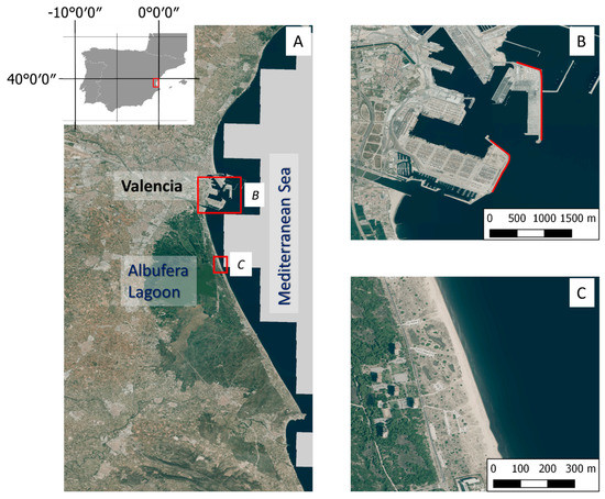
Figure 2.
(A) Detail of Valencia and the Lagoon of the Albufera at the Eastern coast of Spain. (B) Port of Valencia. The red lines are the rigid segments taken for the evaluation of the algorithm; the reference lines are fixed along every date. (C) Detail of part of the sandy beach of El Saler; the reference shorelines are surveyed with GPS at specific dates.
3. New Sub-Pixel Methodological Solution
The method described in this work start from a rough shoreline at the pixel level for each of the Landsat scenes that defines the set of initial pixels where the analysis starts. Note that this initial line can be obtained in various ways such as the thresholds implemented in [20,49,50,51]. Any other accessible line can also be used (such as the shoreline provided by the Instituto Hidrográfico de la Marina for the Spanish territory) but usually these are biased in a magnitude about one Landsat pixel (25–35 m). Hence working with adaptable neighbourhoods may be very useful.
In this paper, a thresholding initial shoreline is used following the bimodal nature of the histogram of an infrared band when water and land are both present [27]. The chosen threshold is unique for the whole scene and the line may displace seaward or landward depending on the selection process. This vagueness is irrelevant because the proposed sub-pixel method is intended to manage this effect. In fact, to enhance this, an experiment deliberately biases the initial line by using a wrong initial shore to show the robustness of the methodology.
Moreover, it is important to note that the satellite imagery has a potential error in its georeferencing that will directly affect the positioning of the shoreline when comparing these against the GPS lines (as shown in [35]). Thus, a preliminary process has been implemented to georeference the Landsat images by computing the Fourier cross-correlation through a PNOA orthophoto of the study site. Once this error has been minimized to less than 0.1 pixels, we consider it as negligible.
3.1. A New Method to Define an Adaptive Window for Shoreline Location Using Divided Differences
Given a pixel that contains a part of the initial shoreline and whose centre has the coordinates , the sub-pixel shoreline is calculated through a curve that approaches around that pixel. Moreover, the method has to be sufficiently robust that if the true shoreline does not pass within that pixel and it passes through neighboring pixels then it will be able to calculate the sub-pixel shoreline where appropriate. Therefore, the potential shoreline solution can be found in the pixel and the analysis window around that pixel. The method described hereafter computes a two-dimensional polynomial expression around each pixel-level shoreline. From this expression, the shoreline is assumed to be on the inflexion line with the largest gradient. As it is obtained mathematically, so a sub-pixel precision is reached. This involves creating a window around each pixel that contains the shoreline and, the divided differences are used for that purpose.
Divided differences are normally linked to the Newton interpolation method. Given a set of “d+1” points (xi, gi) from i = 0 to i = d, it is known that there is only one polynomial of degree less than or equal to “d” that passes through those points. Newton proposed a method in which the polynomial had the following form:
It can be seen that g0 and the different terms G[x0,…] are numbers that multiply , term that gives the powers of x in order to define the polynomial. To calculate these parameters, a table of forward divided differences such as in Table 1 is calculated from the set of points.

Table 1.
Forward divided differences table using set of points (xi, gi) from i = 0 to i = d.
Kth order differences refer to the forward divided differences using (k+1) successive points. For the sake of simplicity, in the following we refer to divided differences considering the smallest index and the number of points within. Somehow, each divided difference means a new term must be included in the polynomial. For example, the line that joins the first two points follows the expression:
The slope between both points is equal to the first divided difference . From that point, if a second degree (related to curvature) is needed, a non-zero value will appear at the second order divided differences column: .
In this paper, the table of divided differences is not used to create the interpolating polynomial but to find the best stencil that detects the transition between land and sea. Figure 3 shows an example using DN in a set of nine pixels in which the shoreline is located. A profile with y = constant is considered so that X-values are pixel coordinates and G represents the DN at each pixel. To show the effect of the DN values, X-coordinates are transformed to a scale between 1 and 9. A pixel with X = 5 is the initial shoreline pixel. The objective for this example is to locate the best stencil of four points around that initial shoreline pixel to fit a third-degree polynomial. In the case of a fifth-degree polynomial, we would have to look for stencils with six pixels. For this, an iterative procedure is used, comparing in each step the absolute value of the divided difference in the stencil formed after adding a point to the left or one pixel to the right of the previous stencil.
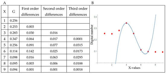
Figure 3.
(A) Example using absolute values of a divided differences table and with X = 5 as the initial shoreline pixel. Values in red are compared in the iterative procedure explained in Section 3.2 to calculate the stencil for the interpolating polynomial, choosing in each column the maximum for such red values. (B) Interpolating the polynomial using the selected four-pixel stencil.
Thus, in each column we only compare the absolute value of the divided differences marked in red in Figure 3A. First, row numbers 5 and 6 in the column of the first order differences are compared—they mean the slope on the stencils {4,5} (0.091) and {5,6} (0.142). The divided difference of the largest module is chosen (which is the row number 6) as we are looking for the largest gradient around the initial point. Row numbers 6 and 7 (of the first and second columns correspondingly) are then compared. They mean the weight of needing a second term of the polynomial at the stencils {4,5,6} and {5,6,7}, respectively. This time the divided difference of the largest module corresponds to row number 7. Finally, in the column of the third order differences, row numbers 7 and 8 are compared. They correspond to a third term of the polynomial at the stencils {4,5,6,7} and {5,6,7,8}. This third divided difference chooses the row 7 (which is calculated over the stencil formed by the {4,5,6,7} X-values) as the best stencil to define the interpolating polynomial around the initial shoreline pixel (X = 5) drawn in Figure 3B.
This idea is extended to two dimensions. Once the pixel-level shoreline is located, the main direction is known. In the data in this paper, the beach follows a north-south direction, and this is the first direction to be analysed. Throughout it, the divided differences are used to select the stencil but with the constraint that the initial pixel will never be located at an extreme of the stencil. Once this stencil is found (in blue in Figure 4), the same process is repeated in the perpendicular direction and for each of the pixels selected previously (in orange in Figure 4). Figure 4 shows how for the same initial pixel, in a coast with a north-south main direction, an initial stencil is found (in blue) of four or six pixels (Figure 4A,B, respectively) by using divided differences in the Y-coordinate.
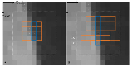
Figure 4.
Examples of the adaptive analysis window corresponding to the initial shoreline pixel () marked with a white cross and shown over a part of an SWIR1 band-L7 image taken on 14 September 2016. The remaining pixel centres of the rough initial shoreline at pixel level are marked with white dots. This line crosses the analysis window from north to south along the Y-axis. The analysis of divided differences is made on the pixels contained within the discontinuous 9 × 9 white square. The window in (A) is composed of a set of 16 pixels (four points each direction) used in a third-degree 2D interpolation, and in (B) by 36 pixels (six points each direction) used in a fifth-degree 2D interpolation. The selected set of pixels along the Y-axis and X-axis is bounded in blue and orange, respectively.
Perpendicularly to each pixel of this initial stencil, the divided differences are used again at their perpendicular directions resulting the stencils marked in orange. In this particular case, the resulting windows in Figure 4A,B will be used for computing, respectively, a third or a fifth-degree two-dimensional polynomial. It must be noticed that those windows are asymmetric because it is impossible the initial pixel to be in the middle of the window having considered an even number of pixels in each direction. Moreover, as stated previously, none of the pixels in the first stencil, coloured in blue, can be located at an extreme edge of its particular stencil.
Small changes in the DNs of the image for a fixed value of Y, as happens in Figure 5 in two consecutive profiles, can lead a very different set of X-axis points being chosen to form the analysis window. This is the advantage of an adaptive window because otherwise when using a fixed and symmetric window around the initial shoreline pixel such as [27], those pixels near the maximum radiometric difference for each single Y-profile cannot be considered. Thus, the interpolating polynomial will pass through those pixels determining the accurate sub-pixel shoreline where the maximum gradient module is reached. As expected and shown in Figure 5, this inflection point will be fairly close to the X-value of the initial shoreline pixel.
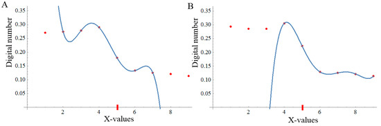
Figure 5.
Two different fifth-degree interpolating polynomials (blue curves) can be seen with the choice of the six-pixel set of Figure 4B (bounded in orange) corresponding to the profiles y = in (A) and y = in (B). Both profiles are indicated with an arrow in Figure 4B. Red dots represent the nine DNs of the entire profile intervening in the search for the set with the maximum radiometric variation in the X-axis (from land to sea pixels). The initial shoreline pixel is in fifth position (red dash). For simplicity, X-coordinates are transformed to a scale of between 1 and 9.
Although this paper considers 2D polynomials of third and fifth-degree, the following procedure may be applied to obtain a general polynomial considering “” as the polynomial degree. Being the initial shoreline pixel center, the analysis window to define the two-dimensional -degree interpolating polynomial is formed by number of pixels. Therefore, such adaptive window is found with the following conditions:
- The points must be included since we estimate that the shoreline passes through the pixel centred in or nearby. This pixel is not expected to be in a corner of the window in the direction of the Y-axis when the maximum radiometric variation occurs.
- A new pixel is added to the previous pixels in the Y-direction by choosing between the two contiguous neighbours, and so after the incorporation of the new pixel, the maximum radiometric variation takes place in the chosen stencil. Thus, we choose between one of these two sets of points or by selecting the set that responds to the maximum fourth-order divided difference in absolute values. We then denote by the smallest index of the Y-coordinate.
- A similar procedure is applied with higher interpolation orders. If then the stencil is formed by an iterative process that begins with these points . A new one is then added to the stencil (until reaching the set of points) by choosing between the two contiguous neighbors, so that the new stencil leads to the maximum variation linked to the maximum divided difference absolute value.
- For each fixed value of the stencil now has to be constructed in the X-direction through an iterative process starting with the point and until reaching the set of points. The choice is made again between the two contiguous neighbors when looking for the maximum divided difference absolute value.
3.2. Definition of the Polynomial Surface in Lagrange Form
Considering “” as the polynomial degree, once each adaptive window is found around each initial pixel, the two-dimensional polynomial that fits the DN values must be found. This polynomial, with (d+1)2 number of terms, will follow the next form:
where the DN of each pixel (G) is function of the pixel coordinates (x,y).
The Lagrange solution follows a similar approach as when obtaining the window in Section 3.1 because it is close to its definition. It is made in two steps that give two parts of the polynomial. When looking for the window, the process began by obtaining the initial stencil at the main direction of the initial shoreline (blue stencil in Figure 4). In the given examples it was along Y-axis. That stencil is used to create the first part of the Lagrange polynomial:
The value of each DN is given by means of in Equation (4). In this case, as the initial stencil takes only values of an specified column i, it remains constant and m moves along the column coordinates from the minimum row near to j (the initial row of the stencil) to , in order to get the degree of the wanted polynomial that decides the size of the window. It means l from to are the rows values of the stencil and are their coordinates. Then, defined in (4) gives a polynomial only dependent on y.
The same way as each horizontal stencil was obtained around the initial vertical stencil (Figure 4). Each one of those stencils (reliant on the y = ym profile considered) can give a new Lagrange polynomial only dependent on x:
Combining the one-dimensional polynomials defined by Equations (4) and (5) we obtain the following two-dimensional polynomial [52]:
In Appendix A, the process of obtaining the polynomial given in Equation (6) is described in detail so that it can be implemented and used by the reader.
3.3. Process to Obtain the Sub-Pixel Inflexion Line
Starting from the Lagrange 2D interpolating polynomials or in Equation (6) considering that d = 3 or d = 5, then the sub-pixel shoreline is calculated using the roots of the Laplacian of these polynomials:
Thus, shorelines are computed by solving the equation (Laplacian equal to zero):
The intersection between the Laplacian and the plane z = 0 within each analysis window offers different candidate curves as a solution. Given a constant Y-value, there are several values of X for which Equation (8) is fulfilled as Figure 6 shows. For the candidate whose polynomial gradient module is maximum, Equation (9) will define the sub-pixel shoreline position for each Y-profile:
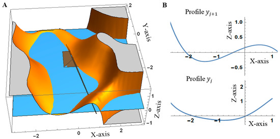
Figure 6.
corresponding to the analysis window shown in Figure 4B. (A) shows the intersections between surface and the plane z = 0 and which are colored in ocher and blue colours, respectively. The initial shoreline pixel is marked by a brown square partially hidden under the plane z = 0; and the GPS or true shoreline is the black line crossing from north to south. (B) shows the Laplacian for two particular Y-profiles (y ) and the intersections with the X-axis—shoreline candidate points.
In addition, it was assessed that the calculated shoreline approximated better to the true reference shoreline nearer the initial pixel than in those further away—although the polynomial surface was obtained by adjusting across the entire analysis window (see example in Figure 6A). Therefore, the sub-pixel shoreline solution to keep for the final result is one of the central Y pixels, leaving aside the two pixels at the extremes where the adjustment may crash due to the irregularity of the neighbourhood.
Moreover, the procedure for obtaining the shoreline position is achieved by dividing its Y-coordinate every 1/4 pixel and then by looking for each sub-pixel shoreline point. For example, a profile is taken every 7.5 meters of distance in the case of Landsat images with a pixel size of 30 meters. Thereby, the shoreline solution equals the density of points obtained with the [27] solution where each pixel of the window had been upsampled in a refined mesh computed with a cubic convolution operator. Other ways to densify may be carried out for other purposes.
Once the sub-pixel shoreline points are obtained for all the analysis windows (as many as initial shoreline pixels), each Y-value will then be several X-solutions due to the overlap between windows. For example, the window that serves as the support for the stencil of the interpolating polynomial overlaps with the window of . Therefore, the final solution for each fixed Y-value is calculated as the average of all the approximate sub-pixel shoreline points obtained through the different initial pixels. Other works such as [33], calculate this average by weighing each solution point according to its distance from the initial pixel (which consequently reduces the RMSE). However, the current paper does not deal with this question as it is focused on assessing exclusively the inner technical core of the sub-pixel methodology (step 2(c) exposed in Section 1). Thus, once tested the improvement in the raw results achieved with the new methodology, subsequent procedures of filtering could be added as in former works to gain precision. At this point, we have a set of unique points that define the position of the shoreline.
The use of an adaptive window in which the initial shoreline pixel is not in the centre of the same may cause an excessive curvature in the calculated shoreline as seen in Figure 7A which oscillates around the true shoreline. This happens to a lesser extent in the case of applying the [27] solution which uses the LSM on a 7 × 7 upsampled window centred in the initial pixel, as we can see in Figure 7B. For this reason, at the end of the sub-pixel calculation process described in this paper (termed aLgr), a smoothening is applied to the set of sub-pixel shoreline points by using the RLOESS technique [53] in function of the percentage of solution points per window.
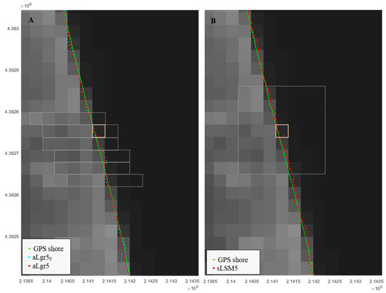
Figure 7.
Sub-pixel shoreline obtained using various methodologies (described next in Table 2) on the 8 October 2016 at El Saler beach and compared with the true shoreline measured by GPS. (A) shows the sub-pixel shoreline solution obtained using successive adaptive windows around each initial shoreline pixel; while (B) uses fixed and symmetrical windows to make the adjustment. (A) also maps an unfinished solution (prior to the smoothening step; aLgr50) that illustrates the curvature effect produced by working with non-centred windows. As an example, a particular adaptive window in (A) and fixed in (B) are bounded in white and both pertain to the initial pixel highlighted in pink. The grid coordinates are: GCS_ETRS89 UTM31N (for an interpretation of the colour references in this figure legend, the reader is referred to the web version of this article).
4. Testing the New Solution: Comparison with Other Interpolation Techniques.
Pardo-Pascual et al. [33]—coming from the methodology of [27]—uses a fifth-degree polynomial expression computed using the LSM and a stencil formed with an upsampled 7 × 7 fixed and symmetric window around the initial shoreline pixel (see Figure 7B). Conversely, the great novelty of this paper is in changing the concept of kernel through the implementation of a smaller adaptive window defined on the pixel-level shoreline that can collect combinations of 16 or 36 pixels (stencils of four or six pixels in each direction) with greater radiometric variations. An adaptive window may select the stencils with which it is constructed to search for the land-water line. This idea assumes that the separation between water and land occurs where the infrared intensity gradient is maximum. Therefore, the shape of the window (see Figure 7A or Figure 4B) may be completely irregular, or even square, if the choice defines it (Figure 4A), but it cannot be centred and symmetric with respect to the initial pixel using an even number of pixels.
Different methodological guidelines are analysed in order to compare the new sub-pixel solution against that used in the technical core of [33]. The analysis window is centred and fixed (symmetric window) around each initial pixel ; or dynamic and non-centered (adaptive window) and in which case all the pixels must be chosen. In addition, a comparative analysis is made that depends on the calculation technique for the polynomial surface, its associated degree, and the corresponding size of the pixel window. To summarize the methodological sub-pixel shoreline solutions—either as a new proposal or as a solution for comparison—the following nomenclatures are shown in Table 2.
Table 2.
The main characteristics of the sub-pixel methodological solutions analysed. The last two correspond to the proposed methodology.
Notice that the solutions applying least squares use a refined mesh to give sufficient equations to the least squares system. sLSM solution is the same as in [33] but this time showing the results without implementing any weighted average to get the final shoreline because solutions want to be compared unprocessed to faithfully appreciate the differences arising only from the sub-pixel method. Once the window is defined, it can be represented by a 2D polynomial surface solved by least squares using an overdetermined system (aLSM3 and aLSM5), or by Lagrange using a non-homogeneous system with a single solution (aLgr3 and aLgr5) and raw pixel data as the current paper proposes. In addition, it is possible to compare aLgr against aLSM or sLSM solutions, as the smoothening carried out in the first solution may equal the cubic convolution process when obtaining the refined mesh in the last two.
All steps proposed in methodology are realized automatically by a created algorithm using Matlab software. Validation process of achieve results has been carried out using the set of 17 sub-pixel shorelines and their respective highly accurate reference lines described in Section 2 of this paper. Section 5 analyses errors calculated through the minimum distance between each sub-pixel shoreline point and the closest respective point of the reference shoreline for each date. Positive and negative distances indicate that the resulting sub-pixel shoreline is biased seaward or landward, respectively.
5. Results
This section presents the results of the new algorithmic solution (aLgr) for obtaining an accurate sub-pixel shoreline regardless of the veracity of an initial pixel-level shoreline. The assessment is completed by comparing this against aLSM and sLSM solutions to show both the importance of the use of the adaptive window and the improvement produced by the Lagrange polynomial interpolation method. Two different series of results are provided—those obtained on a sandy beach and on a port area—and their organization in the following assessments itemizes the methodological differences and improvements in detail.
5.1. Adaptive versus Fixed Search Window
The opening assessment evidences the first challenge of the proposed methodology when working with an adaptive window—meaning the interpolation window defined on the pixel-level shoreline (see Section 3.1).
The two sets of shorelines compared in this section (aLSM versus sLSM) only differ in the window of pixels chosen to adjust the polynomial surface using least squares (see Table 2). sLSM uses a 7 × 7 symmetric window whatever the polynomial degree (3 or 5) is used. aLSM uses an adaptive window (defined according to Equation (A4)) with 16 pixels when looking for third-degree and 36 pixels for fifth-degree. Whatever is the window these solutions follow the same logic: upsampling the kernel and resolution by least squares. A comparative analysis between the shorelines obtained from L7 and L8 images as well as the accuracy per zone is summarized in Table 3—results concerning the aLgr solution will be analysed in the following Section 5.2.
Table 3.
Average (µ), standard deviation (σ) and RMSE values (in meters) describing the precision of different sub-pixel shoreline solutions (of Table 2) for the 17 analysed days (seven L8 and ten L7 images).
Shoreline errors are larger for L7 because, as expected, the SLC-error and consequent data gaps existing on these images sometimes confuse the adjustment surface and cause unrealistic spikes at the ends (as Figure 8 shows). The adaptive window does not have enough pixels with values to adapt to the maximum gradient direction around the ends of each L7 shoreline stretched between the gaps (even with the refined mesh).
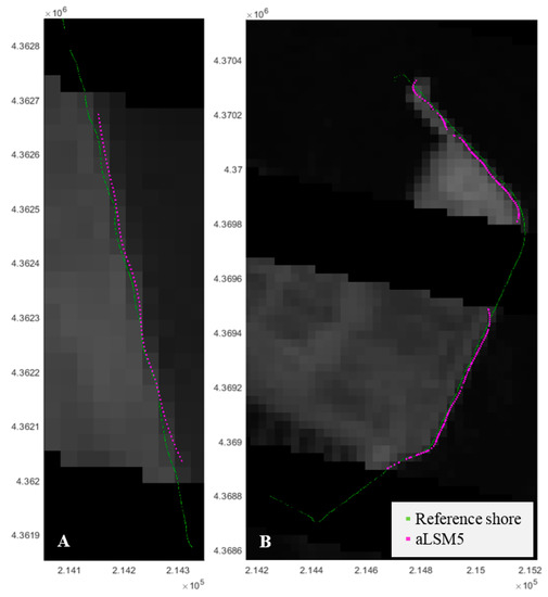
Figure 8.
Local examples of the sub-pixel shoreline solution for 14 September 2016 following the aLSM5 method in both study areas: El Saler beach (A) and the port of Valencia (B). The shoreline solution is mapped above its corresponding L7 image (SWIR1 band) and compared with the true shoreline used as reference, as measured by GPS when the satellite passed overhead in (A) and digitalized over a high-resolution orthophoto in (B). The grid coordinates are: GCS_ETRS89 UTM31N.
Results in the beach area indicate that although shorelines are biased seaward, the use of an adaptive window significantly reduces this trend and the shoreline is defined with a mean horizontal error (µ ± σ) of 4.50 ± 7.6 m and 5.98 ± 5.53 m by adjusting respectively a third (aLSM3) or fifth-degree (aLSM5) polynomial. In the port area, the RMSEs are generally worse because the standard deviations are greater and show a very heterogeneous error distribution that causes a flattening of their histogram. This fact responds to the greater radiometric variation found in the terrestrial part of the port area than in the sandy beach site where the numbers remain more homogeneous—as anticipated by [33]. Moreover, many negative errors indicate a slight landward bias of the shoreline and affect the average error by reducing it to values near zero.
The freedom to work with adaptive windows ensure that these recreate the location with the maximum radiometric variations. Consequently, the search for the sub-pixel shoreline position will be made in the optimal neighbourhood, improving the accuracy of the results. However, the second challenge of the proposed methodology is analysed in next section.
5.2. Benefits of the Complete Solution through the Lagrange Interpolator Polynomial
Working with the discussed adaptive window, this section evaluates the solvency of the complete sub-pixel shoreline solution (aLgr)—performed with the Lagrange interpolator polynomial as described Section 3.2—by comparing against the least squares solution (aLSM). The mathematical difference between both is based on the fact that least squares uses the window with the DNs previously upsampled in a refined mesh whereas Lagrange uses the raw values to carry out the adjustment. Therefore, Lagrange polynomial coincides in the centre of each pixel with the real DN of the image while LSM computes the polynomial that passes closest to the interpolated values.
Looking at the differences between aLSM and aLgr solutions (see errors in Table 3) reveals that the shoreline is more accurate and precise when choosing the second option. This shoreline solution, independently of the calculated polynomial degree, has an overall seaward bias of less than 3.5 m in the beach area and less than 1.8 m in the port area. Moreover, 2.5 m of RMSE difference between both solutions is found in all cases and, the histogram of the aLgr shoreline errors show a more marked symmetry than the rest (the highest relative frequency is found within the 0–5 m interval), thus evidencing the precision and robustness of the new sub-pixel solution. Differences between the errors when working with L8 or L7 data are again noticeable with a bias of 1.79 ± 2.78 m and 4.38 ± 5.66 m respectively for aLgr5; and of 2.01 ± 2.87 m and 4.46 ± 5.06 m, respectively, for aLgr3. Large errors of L7 cause a general increase in the RMSE of all methods.
According to Fisher’s least significant difference (LSD) procedure [54], the multiple comparison technique determines that aLgr and aLSM methodologies work differently, and so their mean shoreline errors are significantly different with a 95% confidence. See that Figure 9 clearly differences these two families of data: aLgr0 and aLgr (pre- and post-smoothing) vs. aLSM. Therefore, this test also proves that the smoothening proposed in the last step of our methodology (aLgr)—described in Section 3.3—far from changing the meaning of the sample, significantly reduces the variability of the data by removing outliers—the same effect was achieved when upsampling with cubic convolution in aLSM and sLSM solutions. Before the smoothening step, the mean shoreline error in the beach area was 3.00 ± 7.34 m with a fifth-degree (aLgr50) and 3.18 ± 7.78 m with a third-degree (aLgr30). This was followed by 3.31 ± 4.47 m and 3.45 ± 4.16 m for the fifth and third-degree solutions respectively (aLgr5 and aLgr3). These results—summarized in Figure 9—confirm the usefulness of the smoothening step to reduce the standard deviation of the errors without altering the meaning of the mean error.
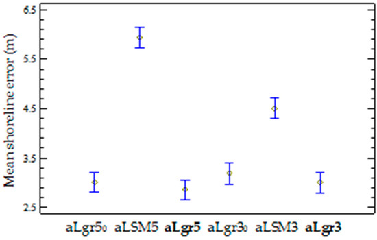
Figure 9.
Mean-value chart with the Fisher LSD intervals at the 95% confidence level in Fisher’s test. The sub-pixel shoreline errors shown correspond to the aLgr0 (prior to the smoothening step), aLSM solutions, and aLgr (which is highlighted in bold for being the proposed methodology) by using a third or a fifth-degree in the polynomial solution. These latter solutions are mapped in Figure 7 for a specific day.
5.3. Resistance of the Methodology against an Inaccurate Initial Shoreline
This section evaluates how the sub-pixel techniques deal with the vagueness of the initial shoreline at pixel level so that final accuracy is not affected. To carry out this assessment, the input shoreline is displaced one pixel landward and seaward from its original location and the different sub-pixel shoreline solutions are obtained to evaluate how these would fix the deviation.
Despite the fact that the initial pixel is expected to be too coarse and does not contain the real shoreline, the sLSM results indicate that the fixed 7 × 7 kernel is extensive enough to cover several pixels of land and water but not equitably. The inflection point of each polynomial surface defining the shoreline may be ambiguous in this scenario. Moreover, and as the large errors in Figure 10 show, it seems that the third-degree adjustment surface (sLSM3) cannot faithfully represent the complexity of the terrain and is less successful in defining the shoreline when just comparing maximum and minimum relatives. Using a fifth-degree polynomial (sLSM5) the sub-pixel shoreline is a little better but still inaccurate with an RMSE of 6.72 m and 11.4 m—depending on whether the rough shoreline pixel was displaced seaward or landward. The methodology of [27] or [33] had not been tested yet coming from a mistaken initial pixel-level shoreline. Nevertheless, the sLSM observations here analysed are in agreement with its implicit notions where the 7 × 7 kernel intended to ensure that the inflexion shoreline was captured around the initial pixel-level solution, and the fifth polynomial degree had enough curvatures to draw the reality of the kernel.
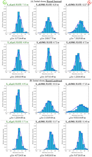
Figure 10.
Histograms representing the density function of the sub-pixel shoreline errors in the beach area depending on the bias of the pixel-level shoreline—seaward (A) or landward (B)—and the methodology used. A normal density function using the average (µ) and the standard deviation (σ) of the data is also considered by leaving underneath a total area of one.
Proceeding with the results of the methodological proposal of this paper, Figure 10 shows first how the choice of an adaptive window with the aLSM solution helps in the search for an accurate shoreline when the initial pixels are wrong. The polynomial surface adapted to these nominated pixels more accurately represents reality. Then, this approach—plus the use of Lagrange with the raw data—leads to an accurate shoreline biased 2.85 ± 3.98 m for S_aLgr5 and 4.07 ± 4.01 m for L_aLgr5, starting accordingly with a seaward or a landward initial shore. The histograms of Figure 10 clearly manifest, from right to left, the advances achieved—after implementing each methodological step—until reach the complete solution (results highlighted in green colour). Separating the previous errors as they come from L8 and L7 images, we got, respectively, a mean horizontal error of 1.42 ± 2.62 m and 3.85 ± 4.94 m for S_aLgr5 and of 2.53 ± 2.64 m and 5.14 ± 4.96 m for L_aLgr5.
Note that despite the less accurate sLSM solutions these seem to improve if the input pixel-level shoreline biased seaward (1.23 ± 6.6 m vs. 9.67 ± 6.05 m—overall mean horizontal errors of S_sLSM5 and L_sLSM5 solutions). This means that the initial pixels are located in the sea, and consequently, more pixels with radiometric values close to zero correspond to sea levels. The adjustments carried out and mapped in Figure 11 for 2 June 2016, prove that generally in each profile along the X-axis from land to sea where there is more water than land pixels, the inflection point-potential shoreline solution is found first (Figure 11A). Conversely, in a profile with more land than water pixels, the sequence of high radiometric values delays the fall in the adjustment polynomial moving the shoreline solution seawards (Figure 11B). However, as expected, when using the proposed aLgr method the differences between both solutions—biased seaward and landward—are minor because the adaptive window matches the correct proportion of land and sea pixels in any case and the shoreline is more accurately defined (also confirmed seeing Figure 13). In particular for 2 June 2016, S_sLSM5 and L_sLSM5 solutions define the shoreline with a bias of –0.65 ± 3.71 m and 7.51 ± 3.54 m; while S_aLgr5 and L_aLgr5 solutions define it within 0.88 ± 1.96 m and 2.28 ± 2.17 m, respectively.

Figure 11.
Map with sub-pixel shoreline solutions for 2 June 2016 of El Saler beach shown over the corresponding L8 (SWIR1 band) image. These are compared with the GPS shoreline representing the same instantaneous water line (continuous green line). The sub-pixel methodological process starts from an initial shore (whose pixels are tagged in yellow) biased seaward (A) and landward (B). Red points are computed with sLSM5 method and black points with aLgr5 method. The grid coordinates are GCS_ETRS89 UTM31N.
6. Discussion
Assuming that the shoreline is the inflexion line between the brighter and darker (land and water) pixels in the infrared bands, one of the main problems in the refinement process is the accuracy of the initial pixel-level shoreline from which the refinement starts. At the same time, even when that line is properly located, a fixed kernel around a specific pixel may not be the best to obtain the sub-pixel land-water inflexion (for example in diagonal shorelines or irregular landforms, such as groins). The methodological solution described in this paper is thought to deal with both problems. While to date, squared and symmetric kernels around the initial solution were used, it has been shown how to apply the concept of divided differences to obtain worthwhile asymmetric and adaptive windows.
By separately analysing every step of the new sub-pixel solution, the usefulness of the method is evaluated. Firstly, in Section 5.1, the wisdom of using an adaptive window is assessed by comparing the aLSM and sLSM solutions (which only differ in the window of pixels chosen to adjust the polynomial surface using least squares). Results in the beach area indicate that simply by using an adaptive window instead of a fixed window, the shoreline is defined more accurately (refer to Table 3). Through the aLSM5 solution it is achieved a mean horizontal error of 5.26 ± 3.38 m and 6.18 ± 6.52 m, respectively, for L8 and L7; while through sLSM5 solution the mean errors are 5.35 ± 3.8 m and 6.83 ± 6.58 m, respectively, for L8 and L7. Differences between these last errors and those of [33]—where it was estimated a mean error of 6.5 ± 3.1 m for L8 and 5.05 ± 5.7 m for L7—are due to the last steps of filtering have been omitted in the solutions of the current paper. On the other hand, the results achieved for the port area behave differently and show a large variability in shoreline error due to the DN heterogeneity of the terrestrial part. However, this consequence is reduced with the adaptive solution as Table 3 presented. Mention that in order to reduce the RMSE in obtaining the shoreline, [29] used a polynomial radiometric correction (PRC) trained and evaluated in three particular seawalls, achieving a decrease in RMSE that ranged between 4.59 to 5.47 m. The relation obtained between the radiometric response around the coastline and its bias was not strong (R2 = 0.45) but the little effect was noticeable at this level. However, later [33] refuted it by proving that such a correction was not valid for other sites, so this has not been applied in the results of current paper.
Secondly, the advantage of using the Lagrange interpolator polynomial with the original DN values (aLgr) compared to least squares in a refined mesh (aLSM) has also been proved in Section 5.2. The sub-pixel shoreline is more accurate and precise when using the new methodology reaching the RMSE of 5.4 m and 5.56 m (with aLgr3 and aLgr5) instead of the 8.83 m and 8.14 m of RMSE obtained with aLSM3 and aLSM5. Working without altering the original image is a positive point because uncontrolled upsampling can lead to problems and generate outliers. Moreover, computation without upsampling is made using a non-homogeneous system with a single solution.
For both study areas, the results generally show a more accurate shoreline using a fifth-degree polynomial (Table 3). It seems that the polynomial surface with a large window of 36 pixels more faithfully represents the reality in our study sites and adjusts better. However, this is very dependent on the coastal morphology (beach width, sand colour, vegetation near the beach, etc.) which affects the radiometric response. The analysis window and adjustment degree is expected to be lower as the dimensions of the beach are smaller—so that the method does not become confused with the radiometry of non-beach elements. Otherwise, if the pixels of the initial shoreline at pixel level are not accurate enough, a small analysis window may not cover an extension of water and land that is representative enough to carry out the adjustment when searching for an accurate sub-pixel shoreline.
The least (sLSM5) and the most (aLgr5) accurate methodologies of those analysed are mapped for two particular dates and compared against their reference GPS shorelines in Figure 12. Using the aLgr5 solution, the shoreline is precisely defined with an average error of 1.54 ± 2.59 m and 3.97 ± 2.73 m for both 18 and 9 June 2016 respectively. Note that GPS and sub-pixel shorelines in Figure 12 move in the same direction between dates.
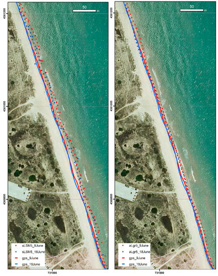
Figure 12.
Coastal segment of El Saler beach where different shoreline solutions are shown for 9 and 18 June in red and blue respectively. The GPS shorelines are represented with lines and the sub-pixel shoreline solutions with dots (sLSM5 and the aLgr5). Solutions painted on an orthophoto taken from 2015 PNOA sources. The grid coordinates are GCS_ETRS89 UTM30N.
Other experiments made in the paper and summarized in Figure 13 prove how the proposed methodology enables accurately establishing the sub-pixel shoreline even starting the process from a rough pixel-level shoreline wrongly biased landward or seaward. Figure 13A show how converging solutions are obtained for any initial pixel shoreline and for each particular analyzed day. The sub-pixel shorelines define with a RMSE of 4.89 m (S_aLgr5) and 5.71 m (L_aLgr5) by starting with a seaward and landward biased initial shores (as already advanced Figure 10)—results in line with the 5.56 m of RMSE obtained when starting with a centred line supposedly located in the correct place. However, if the sub-pixel refinement is attempted with fixed windows as in [33], the final solution will be very conditioned by the precision of the pixel-level shoreline leading to inaccurate results like Figure 13B presents.
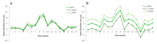
Figure 13.
Mean shoreline error obtained for the 17 analysed days in the beach area by applying both aLgr and sLSM solutions respectively in A and B (accurate and inaccurate results). Small crosses and circles as markers represent L7 and L8 data accordingly. The three sub-pixel shoreline shown have been obtained with the initial pixel-level shore centred (aLgr5 and sLSM5), biased seaward (S_aLgr5 and S_sLSM5) and landward (L_aLgr5 and L_sLSM5).
One of the problems posed by [29]—with same methodological premises as sLSM solution—is the difficulty of defining the shoreline where the coast presents sudden inflections as happens on beaches segmented by groins (sLSM5 solution in Figure 14 exemplifies this distorting effect). Thus, in order to know how the aLgr proposed algorithmic solution responds to this, an additional test is carried out on a beach of such characteristics—south and contiguous to the port of Valencia. Results prove that this methodology clearly reduces the effect of the inflection by avoiding significant errors next to the base of the groin.
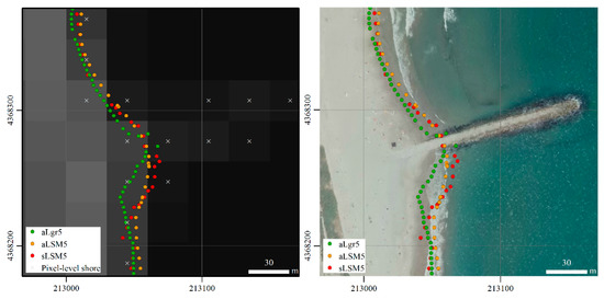
Figure 14.
Map of a groin area with different sub-pixel shoreline solutions obtained for 2 June 2016 displayed on its corresponding L8 image on the left, and on a generic orthophoto (2015 PNOA sources) on the right. The grid coordinates are GCS_ETRS89 UTM31N.
7. Conclusions
This paper has described a new methodology to search for the sub-pixel shoreline from freely available mid-resolution satellite images. A valuable solution to provide accurate coastal information for the improved planning and management of worldwide coastal resources.
The main novelty, compared with other methods previously described in the literature, lies in the definition of an adaptive mathematical window where an algorithm looks for reaching the sub-pixel accuracy by collecting the set of points with the maximum radiometric variation. The proposed method does not alter the original image and works with the raw image data to recreate the land-water surface through the Lagrange interpolation polynomial. It focuses on the sub-pixel refinement process carried out on a pixel-level shoreline—obtained from the image in various ways or be any available line—whose reliability will not condition the precision of the final sub-pixel solution. The objective is then to obtain a two-dimensional piecewise interpolating polynomial around each of its pixels. The shoreline is assumed to be in the inflexion line with the largest gradient, and so sub-pixel precision is obtained mathematically. In contrast to other sub-pixel methodologies [33] where the support window of the polynomial is understood as a fixed squared and symmetric kernel around each pixel, the concept in this work has changed. A new asymmetric solution is described based on the concept of divided differences to find the land-water transition. The adaptive window then collects combinations of 16 or 36 pixels with the greatest radiometric variations for interpolating (depending on the polynomial degree). Once the window is defined, the 2D polynomial surface is solved by the Lagrange interpolating polynomial and its Laplacian roots are calculated to obtain the sub-pixel shoreline points. The compilation of all the sub-pixel solutions for each particular kernel leads to the resulting shorelines analysed in this paper (solutions shown without any weighting average or filtering techniques applied).
The 2D polynomial expression could also be obtained by using least squares. Third and fifth degree polynomials have been used with a previous kernel upsampling to increase the number of equations in the least squares system. However, it has been shown that, avoiding the upsampling drives to more precise and less biased results. At the same time, the adaptive kernel lets to work with the exact number of pixels needed to fit the 2D polynomials. In these cases, not only least squares can be used and the 2D Lagrange interpolator polynomial has been proposed.
The new methodology (aLgr) has been applied to two very different coastal areas (a sandy beach and a segment of the port of Valencia) to analyse how their inherent differences may affect the method. A set of 17 Landsat images (L7 and L8) was used to extract the shoreline. Results have shown the improvement that occurs in estimating the positioning of the sub-pixel shoreline when using the proposed solution, especially in the challenging case of starting with a biased initial pixel-level shoreline. Using the ideas of former methodologies—through the sLSM5 solution—the shoreline was defined with a mean horizontal error not better than 6.0 ± 6.17 m for the beach and 0.71 ± 11.57 m for the port. However, better accuracies are achieved applying the proposed methodology with errors of 3.31 ± 4.47 m and 1.62 ± 6.97 m in those same sites respectively. In particular, and disaggregating these last results for L8 and L7, the error is, respectively, 1.79 ± 2.78 m and 4.38 ± 5.66 m in the beach area, and 1.23 ± 5.62 m and 2.05 ± 8.16 m in the port area. Even more, differences between methodologies exaggerate when the sub-pixel search starts from an initial biased pixel-level shoreline. In these cases, the sLSM5 method is unable to reach a RMSE below the 6.72 m, while the aLgr5 method defines the shoreline with a RMSE of 5.71 m (3.65 m for L8 and 7.14 m for L7) and 4.89 m (2.98 m for L8 and 6.26 m for L7) depending on whether the initial shore was landward or seaward biased.
Author Contributions
Conceptualization: E.S.-G., A.B.-B. and J.A.-C.; methodology: E.S.-G. and A.B.-B.; formal analysis and investigation: E.S.-G. and A.B.-B.; writing—original draft preparation: E.S.-G.; writing—review and editing, E.S.-G., A.B.-B., J.A.-C. and J.E.P.-P.; supervision: A.B.-B., J.E.P.-P. and J.A.-C.; project administration: J.E.P.-P.; funding acquisition: J.E.P.-P.
Acknowledgments
This study is part of the PhD dissertation of E. Sánchez-García, which was supported by a grant from the Spanish Ministry of Education, Culture and Sports (I + D + i 2013–2016). The authors also appreciate the financial support provided by the Spanish Ministry of Economy and Competitiveness (CGL2015-69906-R).
Conflicts of Interest
The authors declare no conflict of interest.
Appendix A. Two-Dimensional Interpolation Process
The methodology to implement the two-dimensional interpolation process described in the paper is detailed below—being the polynomial degree greater than two (d > 2). Assuming that the beach follows a north-south direction, this is the first to be analysed:
(A) Interpolation in the Y-coordinate
(A1) Initially, given the set of discrete values that represent the DN values in the set of three pixels , we define
(A2) The two following third-order divided differences of the function are computed considering that :
From the two possible candidate points, the point with the highest divided difference value will be added to the stencil and used to create the interpolating polynomial of degree . In this way:
- (a) If , then:
- (b) If , then:
The choice will then be made between the following two sets of values from the Landsat image:
(A3) If or each , the following two nth-order divided differences of the function are computed:
In this way:
- (a) If , then
- (b) If , then
In the end: polynomial may be expressed in a Lagrange form as:
For example if then and in the Y-direction we choose one set of DNs between the following:
(B) Interpolation in the X-coordinate
Considering a fixed value of we define the minimum index in the x-coordinate, , using the following iterative process:
(B1)
(B1.1) If then initially, is considered. In this case, the pixel may be at the end of the window in the direction of the X-axis if it this where the maximum variation of the shoreline occurs. This assumption ensures that the sub-pixel shoreline can be correctly defined despite the initial shoreline pixel—around which the analysis is being made—being displaced towards the sea or land by up to three pixels (an equivalent distance of 90 m when working with Landsat images).
For , is supposed to be known. The two following nth-order divided differences are then computed:
- (a) If , then:
- (b) If , then:
(B1.2) If then considering the following pixels
(B2)
For each , is supposed to be known and the two following nth-order divided differences are then computed:
- (a) If , then:
- (b) If , then:
In the end: . For each y we define the following d-degree interpolating polynomial that interpolates along the X-axis considering the stencil
is the unique one-dimensional d-degree polynomial that interpolates the function at point , using the stencil formed by successive points that include . An example of such an adaptive window is shown in Figure 4A,B where for each Y-line a different set of X-coordinates has been selected.
Combining the one-dimensional polynomials defined by (A1) and (A2) we obtain the following two-dimensional polynomial already described in [52]:
This polynomial may be applied in the adaptive window defined by pixels whose centers are:
It can be seen that the value of only depends on the value of the initial pixel; while the values of depend on the line.
References
- Graham, D.; Sault, M.; Bailey, J. National Ocean Service Shoreline—Past, Present, and Future. J. Coast. Res. 2003, 38, 14–32. [Google Scholar]
- Szmytkiewicz, M.; Biegowski, J.; Kaczmarek, L.M.; Okrój, T.; Ostrowski, R.; Pruszak, Z.; Rózynsky, G.; Skaja, M. Coastline changes nearby harbour structures: comparative analysis of one-line models versus field data. Coast. Engineer. 2000, 40, 119–139. [Google Scholar] [CrossRef]
- Furmańczyk, K.; Andrzejewski, P.; Benedyczak, R.; Bugajny, N.; Cieszyński, Ł.; Dudzińska-Nowak, J.; Giza, A.; Paprotny, D.; Terefenko, P.; Zawiślak, T. Recording of selected effects and hazards caused by current and expected storm events in the Baltic Sea coastal zone. J. Coast. Res. 2014, 70, 338–342. [Google Scholar] [CrossRef]
- Baart, F.; Van der Kaaij, T.; Van Ormondt, M.; Van Dongeren, A.; Van Koningsveld, M.; Roelvink, J.A. Real-time forecasting of morphological storm impacts: A case study in the Netherlands. J. Coast. Res. 2009, SI 56, 1617–1621. [Google Scholar]
- Deng, J.; Harff, J.; Zhang, W.; Schneider, R.; Dudzińska-Nowak, J.; Giza, A.; Terefenko, P.; Furmańczyk, K. The dynamic equilibrium shore model for the reconstruction and future projection of coastal morphodynamics. In Coastline Changes of the Baltic Sea from South to East 2017; Springer: Cham, Switzerland, 2017; pp. 87–106. [Google Scholar] [CrossRef]
- Paprotny, D.; Andrzejewski, P.; Terefenko, P.; Furmańczyk, K. Application of empirical wave run-up formulas to the Polish Baltic Sea coast. PloS ONE 2014, 9, e105437. [Google Scholar] [CrossRef] [PubMed]
- Roelvink, D.; Reniers, A.; Van Dongeren, A.P.; de Vries, J.V.T.; McCall, R.; Lescinski, J. Modelling storm impacts on beaches, dunes and barrier islands. CoasT. Engineer. 2009, 56, 1133–1152. [Google Scholar] [CrossRef]
- Kostrzewski, A.; Zwoliński, Z.; Winowski, M.; Tylkowski, J.; Samołyk, M. Cliff top recession rate and cliff hazards for the sea coast of Wolin Island (Southern Baltic). Baltica 2015, 28, 109–120. [Google Scholar] [CrossRef]
- Terefenko, P.; Zelaya Wziątek, D.; Dalyot, S.; Boski, T.; Pinheiro Lima-Filho, F. A High-Precision LiDAR-Based Method for Surveying and Classifying Coastal Notches. ISPRS Int. J. Geo-Inf. 2018, 7, 295. [Google Scholar] [CrossRef]
- Terefenko, P.; Paprotny, D.; Giza, A.; Morales-Nápoles, O.; Kubicki, A.; Walczakiewicz, S. Monitoring Cliff Erosion with LiDAR Surveys and Bayesian Network-based Data Analysis. Remote Sens. 2019, 11, 843. [Google Scholar] [CrossRef]
- Kolander, R.; Morche, D.; Bimböse, M. Quantification of moraine cliff coast erosion on Wolin Island (Baltic Sea, northwest Poland). Baltica 2013, 26, 37–44. [Google Scholar] [CrossRef]
- Pereira, E.; Bencatel, R.; Correia, J.; Félix, L.; Gonçalves, G.; Morgado, J.; Sousa, J. Unmanned air vehicles for coastal and environmental research. J. Coast. Res. 2009, II, 1557–1561. [Google Scholar]
- Lopes, M.; Marques, M.; Coelho, C.; Araújo, A.; Gomes, A.A. Adavantages of using UAVs data to study rocky coasts geomorphology: the case study of the São Paio rocky littoral, Portugal. In Proceedings of the Small Unmanned Aerial Systems for Environmental Research: 5th International Conference, Vila Real, Portugal, 28–30 June 2017. [Google Scholar]
- Moore, L.J.; Ruggiero, P.; List, J.H. Comparing Mean High Water and High Water Line Shorelines: Should Proxy-Datum Offsets be Incorporated into Shoreline Change Analysis? J. Coast. Res. 2006, 22, 894–905. [Google Scholar] [CrossRef]
- Davidson, M.; Van Koningsveld, M.; de Kruif, A.; Rawson, J.; Holman, R.; Lamberti, A.; Medina, R.; Kroon, A.; Aarninkhof, S. The CoastView project: Developing video-derived Coastal State Indicators in support of coastal zone management. Coast. Eng. 2007, 54, 463–475. [Google Scholar] [CrossRef]
- Aarninkhof, S.G.; Turner, I.L.; Dronkers, T.D.T.; Caljouw, M.; Nipius, L. A video-based technique for mapping intertidal beach bathymetry. Coast. Eng. 2003, 49, 275–289. [Google Scholar] [CrossRef]
- Andriolo, U.; Sánchez-García, E.; Taborda, R. Operational Use of Surfcam Online Streaming Images for Coastal Morphodynamic Studies. Remote Sens. 2019, 11, 78. [Google Scholar] [CrossRef]
- Sánchez-García, E.; Balaguer-Beser, A.; Pardo-Pascual, J.E. C-Pro: A coastal projector monitoring system using terrestrial photogrammetry with a geometric horizon constraint. ISPRS J. Photogramm. Remote Sens. 2017, 128, 255–273. [Google Scholar] [CrossRef]
- Holman, R.A.; Stanley, J. The history and technical capabilities of Argus. Coast. Eng. 2007, 54, 477–491. [Google Scholar] [CrossRef]
- Sagar, S.; Roberts, D.; Bala, B.; Lymburner, L. Extracting the intertidal extent and topography of the Australian coastline from a 28 year time series of Landsat observations. Remote Sens. Environ. 2017, 195, 153–169. [Google Scholar] [CrossRef]
- Luijendijk, A.; Hagenaars, G.; Ranasinghe, R.; Baart, F.; Donchyts, G.; Aarninkhof, S. The State of the World’s Beaches. Sci. Rep. 2018, 8, 1–11. [Google Scholar] [CrossRef]
- USGS. Technical announcement: Imagery for Everyone. Available online: https://landsat.usgs.gov/sites/default/files/1f031_7f618-pdf-usgs-landsat-imagery-release.pdf (accessed on 8 May 2018).
- Li, J.; Roy, D.P. A global analysis of Sentinel-2A, Sentinel-2B and Landsat-8 data revisit intervals and implications for terrestrial monitoring. Remote Sens. 2017, 9, 902. [Google Scholar] [CrossRef]
- Boak, E.H.; Turner, I.L. Shoreline Definition and Detection: A Review. J. Coast. Res. 2005, 214, 688–703. [Google Scholar] [CrossRef]
- Gens, R. Remote sensing of coastlines: Detection, extraction and monitoring. Int. J. Remote Sens. 2010, 31, 1819–1836. [Google Scholar] [CrossRef]
- Liu, H.; Wang, L.; Sherman, D.J.; Wu, Q.; Su, H. Algorithmic Foundation and Software Tools for Extracting Shoreline Features from Remote Sensing Imagery and LiDAR Data. J. Geogr. Inf. Syst. 2011, 3, 99–119. [Google Scholar] [CrossRef]
- Almonacid-Caballer, J. Extraction of Shorelines with Sub-Pixel Precision from Landsat Images (TM, ETM+, OLI) [Obtención de Lineas de Costa con Precisión Sub-Pixel a Partir de Imágenes Landsat (TM, ETM+ y OLI)]. Ph.D. Thesis, Universitat Politècnica de València, Valencia, Spain, 10 October 2014. [Google Scholar]
- Ruiz, L.A.; Pardo, J.E.; Almonacid-Caballer, J.; Rodríguez, B. Coastline automated detection and multi-resolution evaluation using satellite images. In Proceedings of the Coastal Zone 07, Portland, OR, USA, 22–26 July 2007 ; pp. 22–26. [Google Scholar]
- Pardo-Pascual, J.E.; Almonacid-Caballer, J.; Ruiz, L.A.; Palomar-Vázquez, J. Automatic extraction of shorelines from Landsat TM and ETM+ multi-temporal images with subpixel precision. Remote Sens. Environ. 2012, 123, 1–11. [Google Scholar] [CrossRef]
- Pardo-Pascual, J.E.; Almonacid-Caballer, J.; Ruiz, L.A.; Palomar-Vázquez, J.; Rodrigo-Alemany, R. Evaluation of storm impact on sandy beaches of the Gulf of Valencia using Landsat imagery series. Geomorphology 2014, 214, 388–401. [Google Scholar] [CrossRef]
- Almonacid-Caballer, J.; Sánchez-García, E.; Pardo-Pascual, J.E.; Balaguer-Beser, A.A.; Palomar-Vázquez, J. Evaluation of annual mean shoreline position deduced from Landsat imagery as a mid-term coastal evolution indicator. Mar. Geol. 2016, 372, 79–88. [Google Scholar] [CrossRef]
- Sánchez-García, E.; Pardo-Pascual, J.E.; Balaguer-Beser, A.; Almonacid-Caballer, J. Analysis of the shoreline position extracted from Landsat TM and ETM+ imagery. Int. Arch. Photogramm. Remote Sens. Spatial Inf. Sci. 2015, 991–998. [Google Scholar] [CrossRef]
- Pardo-Pascual, J.E.; Sánchez-García, E.; Almonacid-Caballer, J.; Palomar-Vázquez, J.M.; de los Santos, E.P.; Fernández-Sarría, A.; Balaguer-Beser, A. Assessing the accuracy of automatically extracted shorelines on microtidal beaches from Landsat 7, Landsat 8 and Sentinel-2 imagery. Remote Sens. 2018, 10, 326. [Google Scholar] [CrossRef]
- Palomar-Vázquez; Jesús Almonacid-Caballer, J.; Pardo-Pascual, J.E.; Sánchez-García, E. Shorex: A new tool for automatic and massive extraction of shorelines from Landsat and Sentinel 2 imagery L–8. In Proceedings of the 7th International Conference on the Application of Physical Modelling in Coastal and Port Engineering and Science (Coastlab18), Santander, Spain, 22–26 may 2018. [Google Scholar]
- Almonacid-Caballer, J.; Pardo-Pascual, J.E.; Ruiz, L.A. Evaluating fourier cross-correlation sub-pixel registration in Landsat images. Remote Sensing. 2017, 9, 1051. [Google Scholar] [CrossRef]
- Liu, Q.; Trinder, J.; Turner, I.L. A comparison of sub-pixel mapping methods for coastal areas. In Proceedings of the XXIII ISPRS Congress, Prague, Czech Republic, 12–19 July 2016; pp. 67–74. [Google Scholar] [CrossRef]
- Liu, Y.; Wang, X.; Ling, F.; Xu, S.; Wang, C. Analysis of coastline extraction from Landsat-8 OLI imagery. Water 2017, 9, 816. [Google Scholar] [CrossRef]
- Liu, Q.; Trinder, J.; Turner, I.L. Automatic super-resolution shoreline change monitoring using Landsat archival data: a case study at Narrabeen–Collaroy Beach, Australia. J. Appl. Remote Sens. 2017, 11, 016036. [Google Scholar] [CrossRef]
- Cipolletti, M.P.; Delrieux, C.A.; Perillo, G.M.E.; Cintia Piccolo, M. Superresolution border segmentation and measurement in remote sensing images. Comput. Geosci. 2012, 40, 87–96. [Google Scholar] [CrossRef]
- Liu, H.; Jezek, K.C. Automated extraction of coastline from satellite imagery by integrating Canny edge detection and locally adaptive thresholding methods. Int. J. Remote Sens. 2004, 25, 937–958. [Google Scholar] [CrossRef]
- Almonacid-Caballer, J.; Pardo-Pascual, J.E.; Ruiz, L.A. Detección automática de la línea de costa con precisión subpíxel en imágenes Landsat 7 con error de bandeado. In Proceedings of the XV Congr. la Asoc. Española Teledetección ” Sistemas Operacionales de Observación de la Tierra”, Torrejón de Ardoz (Madrid), Spain, 22–24 october 2013; pp. 270–273. [Google Scholar]
- Hermosilla, T.; Bermejo, E.; Balaguer, A.; Ruiz, L.A. Non-linear fourth-order image interpolation for subpixel edge detection and localization. Image Vis. Comput. 2008, 26, 1240–1248. [Google Scholar] [CrossRef]
- Harten, A.; Engquist, B.; Osher, S.; Chakravarthy, S.R. Uniformly high order accurate essentially non-oscillatory schemes, III. J. Comput. Phys. 1987, 71, 231–303. [Google Scholar] [CrossRef]
- Shu, C.W.; Osher, S. Efficient implementation of essentially non-oscillatory shock-capturing schemes. J. Comput. Phys. 1988, 77, 439–471. [Google Scholar] [CrossRef]
- Capilla, M.T.; Balaguer, A. A new well-balanced non-oscillatory central scheme for the shallow water equations on rectangular meshes. J. Comput. Appl. Mathem. 2013, 252, 62–74. [Google Scholar] [CrossRef]
- Balaguer, A.; Conde, C. Fourth-order non-oscillatory upwind and central schemes for hyperbolic conservation laws. SIAM J. Numer. Anal. 2005, 43, 455–473. [Google Scholar] [CrossRef]
- NASA. Landsat 7 science data users handbook. Natl. Aeronaut. Sp. Adm. Landsat 186; U.S. Geological Survey (USGS): Greenbelt, MD, USA, 2009.
- Pardo-Pascual, J.E.; Sanjaume, E. Beaches in Valencian Coast. In The Spanish Coastal Systems; Morales, J., Ed.; Springer: Cham, Switzerland, 2019; pp. 209–236. [Google Scholar] [CrossRef]
- Kelly, J.T.; Gontz, A.M. Using GPS-surveyed intertidal zones to determine the validity of shorelines automatically mapped by Landsat water indices. Int. J. Appl. Earth Obs. Geoinf. 2018, 65, 92–104. [Google Scholar] [CrossRef]
- Xu, N. Detecting Coastline Change with All Available Landsat Data over 1986–2015: A Case Study for the State of Texas, USA. Atmosphere 2018, 9, 107. [Google Scholar] [CrossRef]
- Shrivakshan, G.T.; Chandrasekar, D. A Comparison of various Edge Detection Techniques used in Image Processing. IJCSI Int. J. Comput. Sci. Issu. 2012, 9, 269–276. [Google Scholar]
- Balaguer, A.; Conde, C.; López, J.A.; Martínez, V. A finite volume method with a modified ENO scheme using a Hermite interpolation to solve advection diffusion equations. Int. J. Numer. Methods Eng. 2001, 50, 2339–2371. [Google Scholar] [CrossRef]
- Press, W.H.; Teukolsky, S.A. Savitzky-Golay Smoothing Filters. Comput. Phys. 1990, 4, 669. [Google Scholar] [CrossRef]
- Milliken, G.A.; Johnson, D.E. Analysis of Messy Data, Vol. 1; Chapman & Hall/CRC: Boca Raton, FL, USA, 1992. [Google Scholar]


© 2019 by the authors. Licensee MDPI, Basel, Switzerland. This article is an open access article distributed under the terms and conditions of the Creative Commons Attribution (CC BY) license (http://creativecommons.org/licenses/by/4.0/).