Canopy Height and Above-Ground Biomass Retrieval in Tropical Forests Using Multi-Pass X- and C-Band Pol-InSAR Data

Abstract
1. Introduction
2. Study Area and Data
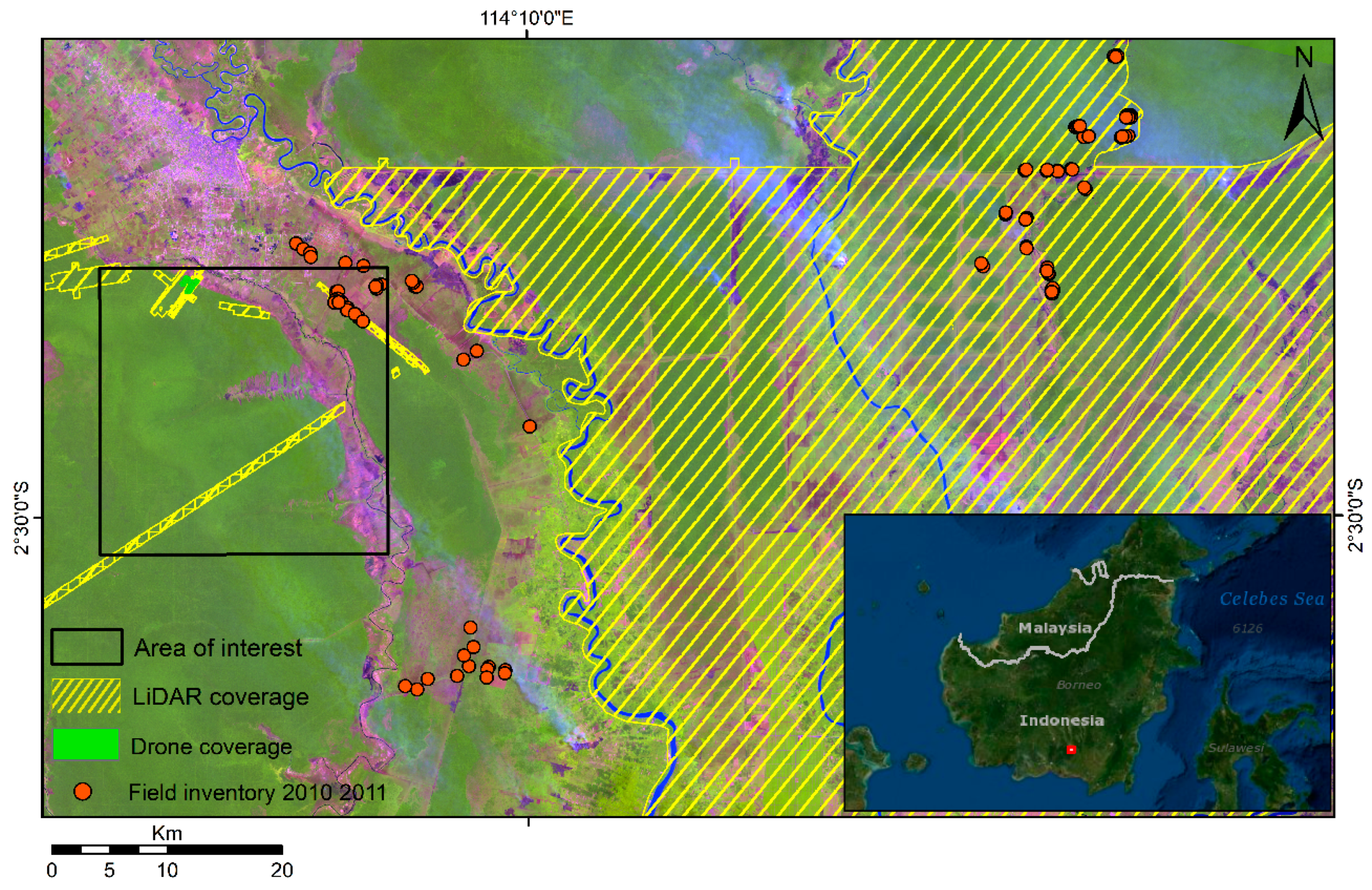
2.1. Study Area
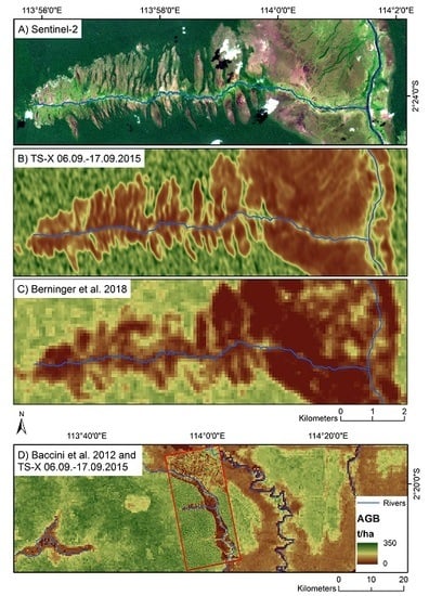
2.2. Reference Data
2.2.1. Field Inventory Data
2.2.2. LiDAR Data
2.3. SAR Data
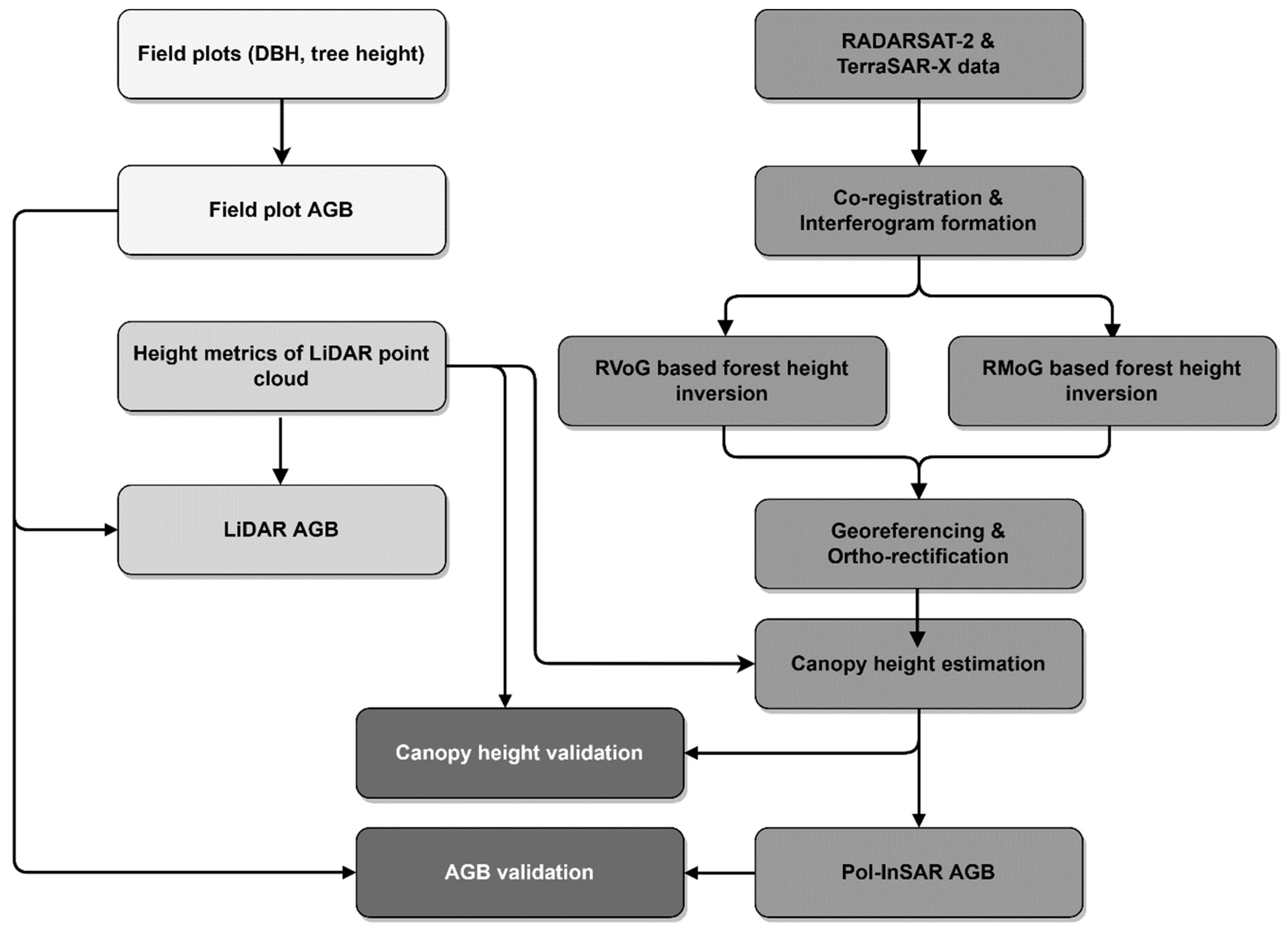
3. Methods
3.1. Extrapolated Reference Data
3.2. SAR Processing
3.3. Canopy Height Estimation
3.4. SAR Based AGB Modelling
3.5. Validation
4. Results
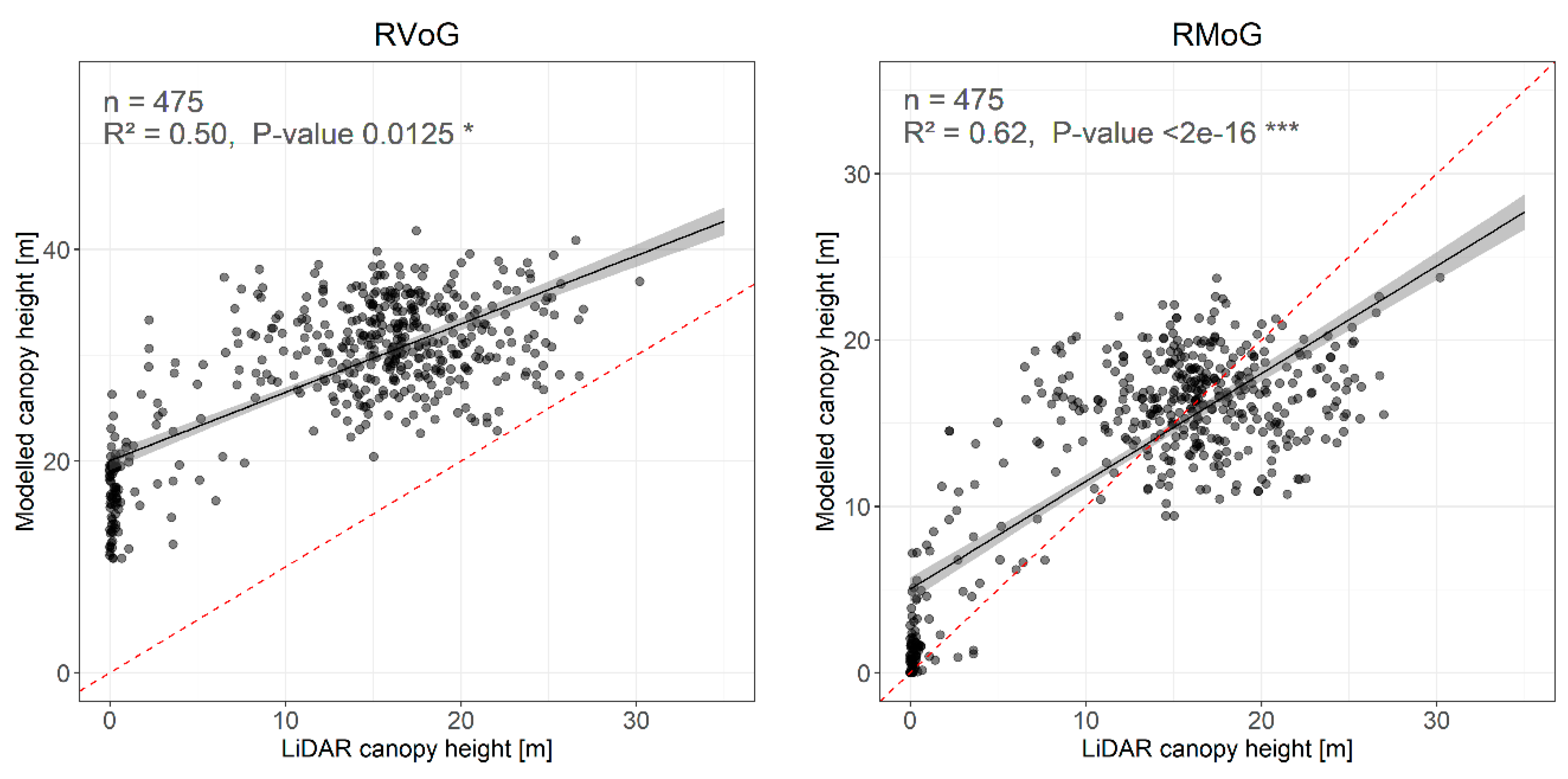
4.1. RVoG vs. RMoG
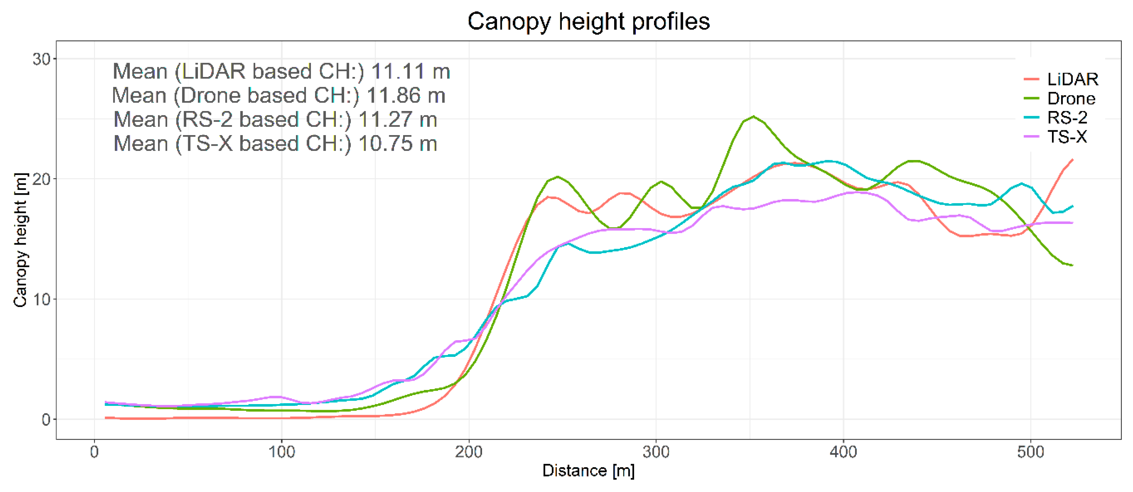
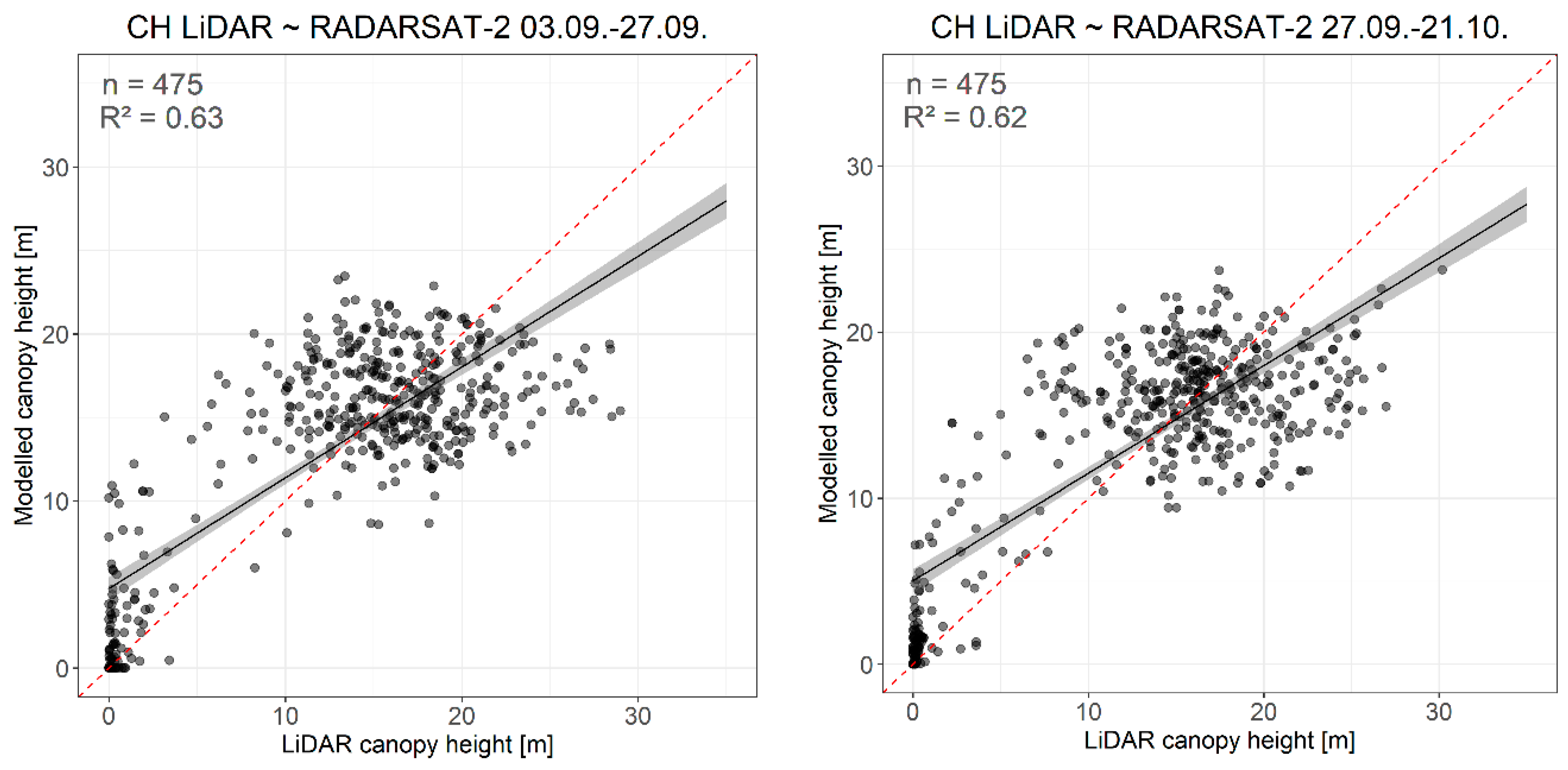
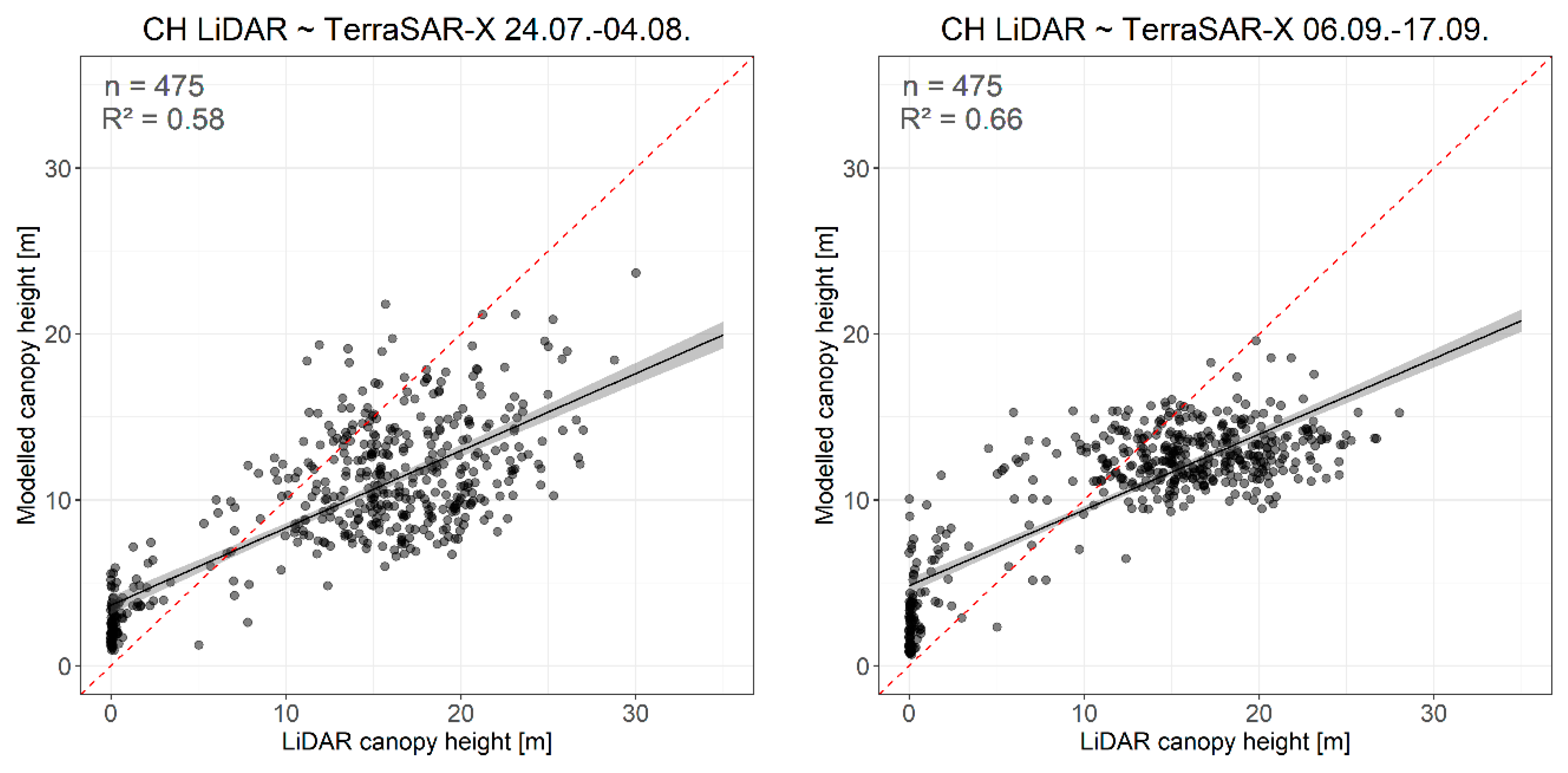
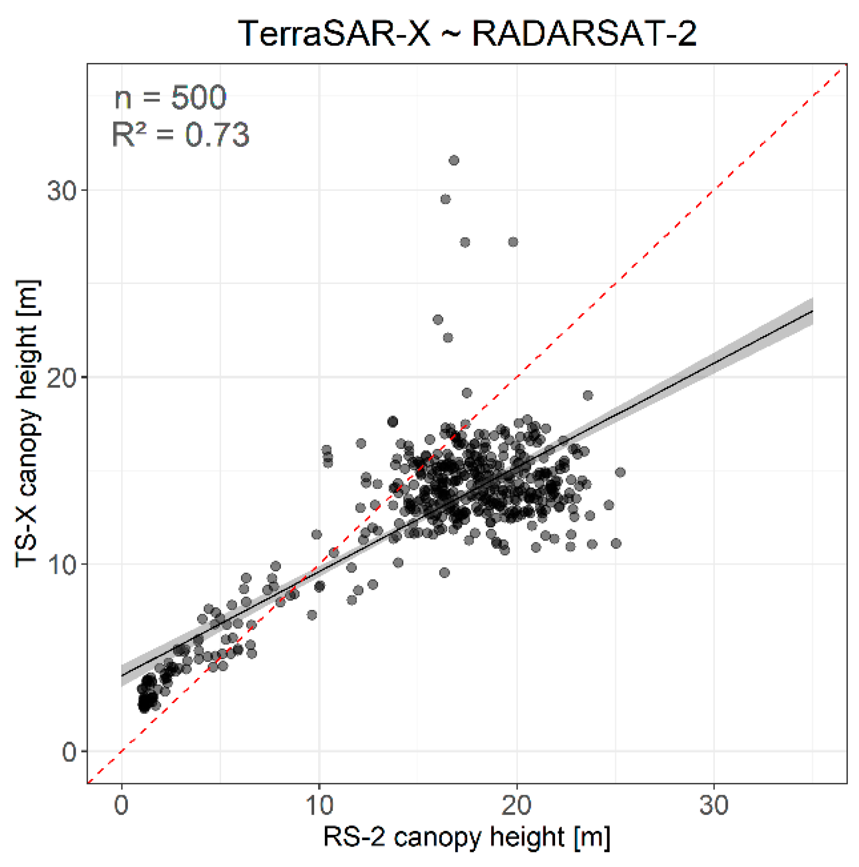
4.2. Canopy Height Estimation
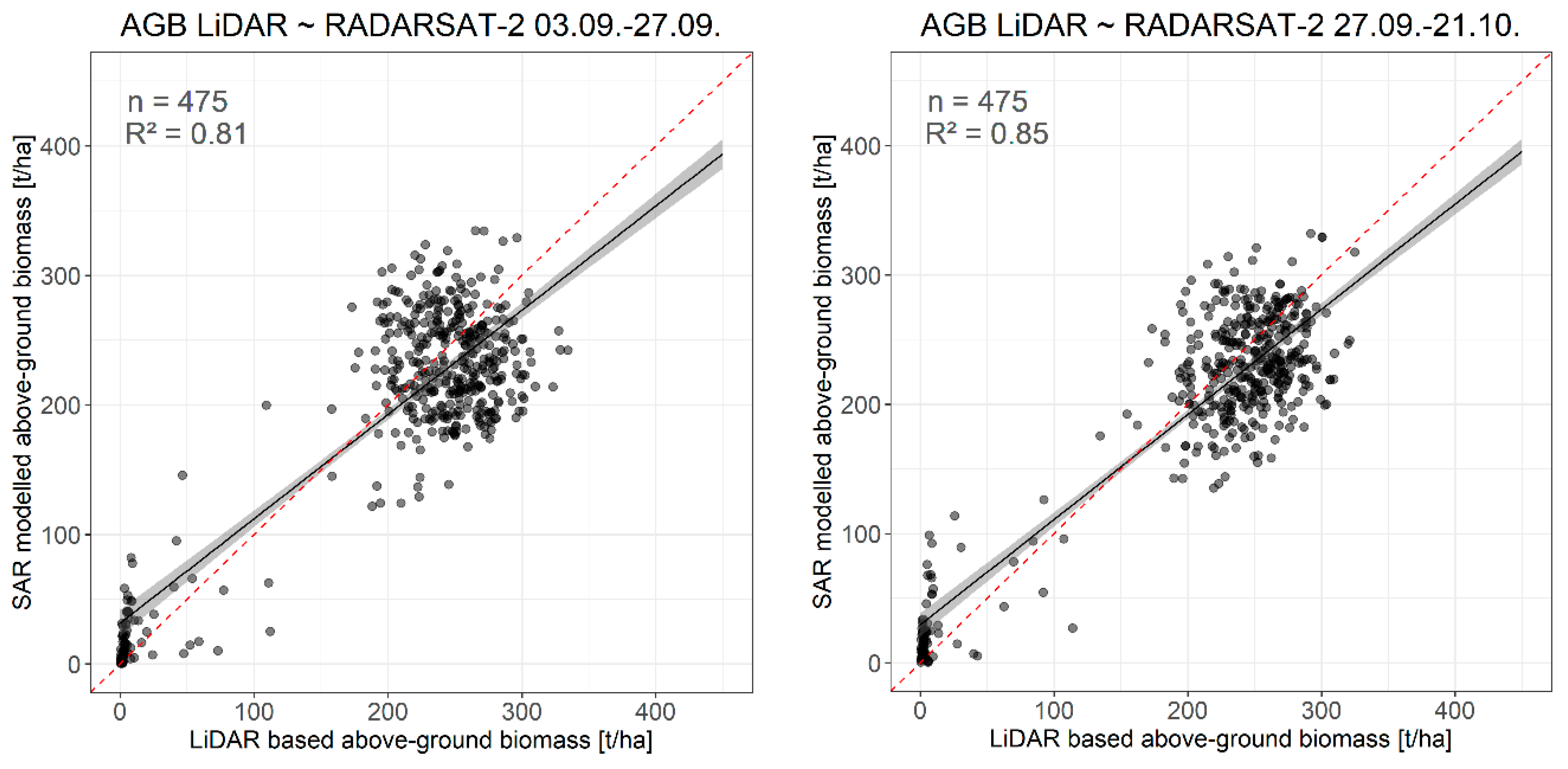
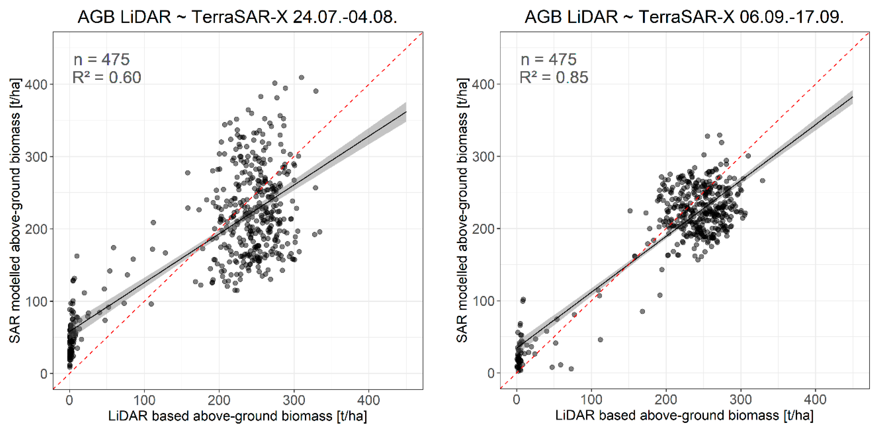
4.3. AGB Estimation
5. Discussion
5.1. Comparison of the RVoG and RMoG Models
5.2. Canopy Height Estimation
5.3. Possible Sources of Error
5.3.1. Acquisition Parameters
5.3.2. Validation Datasets
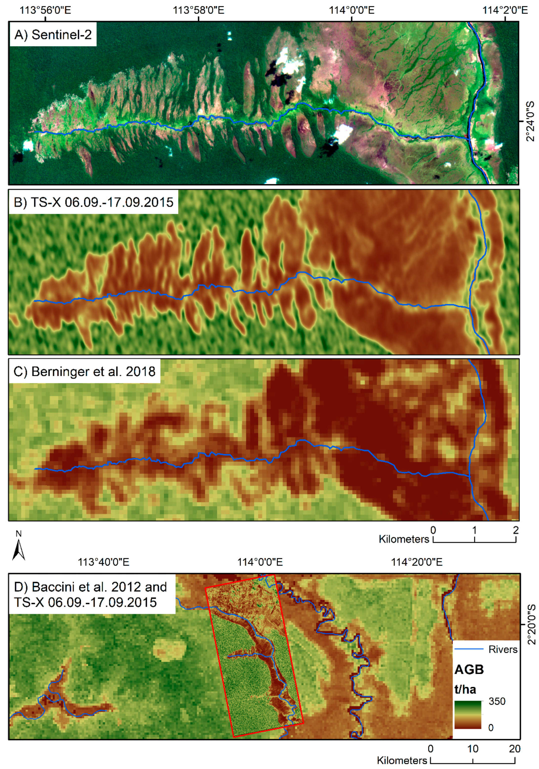
5.4. AGB Estimation
6. Conclusions
Author Contributions
Funding
Acknowledgments
Conflicts of Interest
References
- World Bank Group. Forest Area (% of Land Area): Indonesia. Available online: https://data.worldbank.org/indicator/AG.LND.FRST.ZS?end=2015&locations=IDtart=2015&type=shaded&view=map&year=2010 (accessed on 14 February 2019).
- Pachauri, R.K.; Meyer, L.A. IPCC 2014. Climate change 2014. Synthesis report. Contribution of Working Groups I, II and III to the Fifth Assessment Report of the Intergovernmental Panel on Climate Change; Core Writing Team, Pachauri, R.K., Meyer, L.A., Eds.; Intergovernmental Panel on Climate Change: Geneva, Switzerland, 2015; ISBN 9291691437. [Google Scholar]
- Page, S.E.; Rieley, J.O.; Banks, C.J. Global and regional importance of the tropical peatland carbon pool. Glob. Chang. Biol. 2011, 17, 798–818. [Google Scholar] [CrossRef]
- Jaenicke, J.; Rieley, J.O.; Mott, C.; Kimman, P.; Siegert, F. Determination of the amount of carbon stored in Indonesian peatlands. Geoderma 2008, 147, 151–158. [Google Scholar] [CrossRef]
- Edwards, D.P.; Koh, L.P.; Laurance, W.F. Indonesia’s REDD+ pact: Saving imperilled forests or business as usual? Biol. Conserv. 2012, 151, 41–44. [Google Scholar] [CrossRef]
- Olivier, J.G.J.; Janssens-Maenhout, G.; Muntean, M.; Peters, J.A.H.W. Trends in Global CO2 Emissions: 2015 Report. 2015. Available online: https://edgar.jrc.ec.europa.eu/news_docs/jrc-2015-trends-in-global-co2-emissions-2015-report-98184.pdf (accessed on 26 February 2019).
- Global Canopy Foundation. The REDD Desk. Available online: https://theredddesk.org/countries/search-countries-database?f%5B0%5D=type%3Aactivity&f%5B1%5D=field_project%3A1 (accessed on 7 February 2018).
- Goetz, S.; Dubayah, R. Advances in remote sensing technology and implications for measuring and monitoring forest carbon stocks and change. Carbon Manag. 2011, 2, 231–244. [Google Scholar] [CrossRef]
- FAO. Assessment of the Status of the Development of the Standards for the Terrestrial Essential Climate Variables. 2009. Available online: http://www.fao.org/3/i1238e/i1238e00.pdf (accessed on 6 February 2019).
- Bojinski, S.; Verstraete, M.; Peterson, T.C.; Richter, C.; Simmons, A.; Zemp, M. The Concept of Essential Climate Variables in Support of Climate Research, Applications, and Policy. Bull. Am. Meteorol. Soc. 2014, 95, 1431–1443. [Google Scholar] [CrossRef]
- Koch, B. Status and future of laser scanning, synthetic aperture radar and hyperspectral remote sensing data for forest biomass assessment. ISPRS J. Photogramm. Remote Sens. 2010, 65, 581–590. [Google Scholar] [CrossRef]
- Joshi, N.; Mitchard, E.T.A.; Schumacher, J.; Johannsen, V.K.; Saatchi, S.; Fensholt, R. L-Band SAR Backscatter Related to Forest Cover, Height and Aboveground Biomass at Multiple Spatial Scales across Denmark. Remote Sens. 2015, 7, 4442–4472. [Google Scholar] [CrossRef]
- Schlund, M.; Poncet, F.; Kuntz, S.; Schmullius, C.; Hoekman, D.H. TanDEM-X data for aboveground biomass retrieval in a tropical peat swamp forest. Remote Sens. Environ. 2014, 158, 255–266. [Google Scholar] [CrossRef]
- Asner, G.P.; Clark, J.K.; Mascaro, J.; Galindo García, G.A.; Chadwick, K.D.; Navarrete Encinales, D.A.; Paez-Acosta, G.; Cabrera Montenegro, E.; Kennedy-Bowdoin, T.; Duque, Á.; et al. High-resolution mapping of forest carbon stocks in the Colombian Amazon. Biogeosciences 2012, 9, 2683–2696. [Google Scholar] [CrossRef]
- Asner, G.P.; Flint Hughes, R.; Varga, T.A.; Knapp, D.E.; Kennedy-Bowdoin, T. Environmental and Biotic Controls over Aboveground Biomass Throughout a Tropical Rain Forest. Ecosystems 2009, 12, 261–278. [Google Scholar] [CrossRef]
- Solberg, S.; Astrup, R.; Gobakken, T.; Næsset, E.; Weydahl, D.J. Estimating spruce and pine biomass with interferometric X-band SAR. Remote Sens. Environ. 2010, 114, 2353–2360. [Google Scholar] [CrossRef]
- Englhart, S.; Keuck, V.; Siegert, F. Aboveground biomass retrieval in tropical forests—The potential of combined X- and L-band SAR data use. Remote Sens. Environ. 2011, 115, 1260–1271. [Google Scholar] [CrossRef]
- Duncanson, L.I.; Niemann, K.O.; Wulder, M.A. Estimating forest canopy height and terrain relief from GLAS waveform metrics. Remote Sens. Environ. 2010, 114, 138–154. [Google Scholar] [CrossRef]
- Zhao, K.; Popescu, S.; Nelson, R. Lidar remote sensing of forest biomass: A scale-invariant estimation approach using airborne lasers. Remote Sens. Environ. 2009, 113, 182–196. [Google Scholar] [CrossRef]
- Kronseder, K.; Ballhorn, U.; Böhm, V.; Siegert, F. Above ground biomass estimation across forest types at different degradation levels in Central Kalimantan using LiDAR data. Int. J. Appl. Earth Obs. Geoinf. 2012, 18, 37–48. [Google Scholar] [CrossRef]
- Asner, G.P.; Powell, G.V.N.; Mascaro, J.; Knapp, D.E.; Clark, J.K.; Jacobson, J.; Kennedy-Bowdoin, T.; Balaji, A.; Paez-Acosta, G.; Victoria, E.; et al. High-resolution forest carbon stocks and emissions in the Amazon. Proc. Natl. Acad. Sci. USA 2010, 107, 16738–16742. [Google Scholar] [CrossRef]
- Ballhorn, U.; Jubanski, J.; Siegert, F. ICESat/GLAS Data as a Measurement Tool for Peatland Topography and Peat Swamp Forest Biomass in Kalimantan, Indonesia. Remote Sens. 2011, 3, 1957–1982. [Google Scholar] [CrossRef]
- Jubanski, J.; Ballhorn, U.; Kronseder, K.; Franke, J.; Siegert, F. Detection of large above-ground biomass variability in lowland forest ecosystems by airborne LiDAR. Biogeosciences 2013, 10, 3917–3930. [Google Scholar] [CrossRef]
- Englhart, S.; Jubanski, J.; Siegert, F. Quantifying Dynamics in Tropical Peat Swamp Forest Biomass with Multi-Temporal LiDAR Datasets. Remote Sens. 2013, 5, 2368–2388. [Google Scholar] [CrossRef]
- Sun, X.; Song, H.J. A New Improved Algorithm Based on Three-Stage Inversion Procedure of Forest Height. In Proceedings of the 2015 14th International Symposium on Distributed Computing and Applications for Business Engineering and Science (DCABES), Guiyang, China, 18–24 August 2015; Available online: https://dl.acm.org/citation.cfm?id=2917944 (accessed on 26 February 2019).
- Olesk, A.; Praks, J.; Antropov, O.; Zalite, K.; Arumäe, T.; Voormansik, K. Interferometric SAR Coherence Models for Characterization of Hemiboreal Forests Using TanDEM-X Data. Remote Sens. 2016, 8, 700. [Google Scholar] [CrossRef]
- Lavalle, M.; Simard, M.; Hensley, S. A Temporal Decorrelation Model for Polarimetric Radar Interferometers. IEEE Trans. Geosci. Remote Sens. 2012, 50, 2880–2888. [Google Scholar] [CrossRef]
- Garestier, F.; Dubois-Fernandez, P.C.; Papathanassiou, K.P. Pine Forest Height Inversion Using Single-Pass X-Band PolInSAR Data. IEEE Trans. Geosci. Remote Sens. 2008, 46, 59–68. [Google Scholar] [CrossRef]
- Neumann, M.; Ferro-Famil, L.; Reigber, A. Multibaseline Polarimetric SAR Interferometry Coherence Optimization. IEEE Geosci. Remote Sens. Lett. 2008, 5, 93–97. [Google Scholar] [CrossRef]
- Kugler, F. Pol-InSAR Forest Height estimation at different Frequencies: Oppertunities and Limitations. 2015. Available online: https://elib.dlr.de/102764/1/Dissertation-Florian-Kugler.pdf (accessed on 22 May 2019).
- Hajnsek, I.; Hoekman, D.H. INDREX-II Indonesian Radar Experiment Campaign over Tropical Forest in L- and P-band. In Proceedings of the 2005 IEEE International Geoscience and Remote Sensing Symposium (IGARSS), Seoul, Korea, 29 July 2005; Volume 6, pp. 4335–4338. Available online: https://ieeexplore.ieee.org/document/1525878 (accessed on 30 April 2019).
- Hajnsek, I.; Kugler, F.; Lee, S.K.; Papathanassiou, K.P. Tropical-Forest-Parameter Estimation by Means of Pol-InSAR: The INDREX-II Campaign. IEEE Trans. Geosci. Remote Sens. 2009, 47, 481–493. [Google Scholar] [CrossRef]
- Kugler, F.; Schulze, D.; Hajnsek, I.; Pretzsch, H.; Papathanassiou, K.P. TanDEM-X Pol-InSAR Performancefor forest height estimation. IEEE Trans. Geosci. Remote Sens. 2014, 52, 6404–6422. [Google Scholar] [CrossRef]
- Vyjayanthi, N.; Jha, C.S.; Murthy, M.S.R. Forest Biomass Estimation and Forest Structure Analysis from Multi-Frequency and Multi-Polarization SAR Data. RISAT-JEP. 2017. Available online: https://www.climatelinks.org/file/4121/download?token=WzORdftr (accessed on 22 April 2019).
- Varekamp, C.; Hoekman, D.H. High-resolution InSAR image simulation for forest canopies. IEEE Trans. Geosci. Remote Sens. 2002, 40, 1648–1655. [Google Scholar] [CrossRef]
- Avitabile, V.; Herold, M.; Heuvelink, G.B.M.; Lewis, S.L.; Phillips, O.L.; Asner, G.P.; Armston, J.; Ashton, P.S.; Banin, L.; Bayol, N.; et al. An integrated pan-tropical biomass map using multiple reference datasets. Glob. Chang. Biol. 2016, 22, 1406–1420. [Google Scholar] [CrossRef]
- Page, S.E.; Rieley, J.O.; Wüst, R. Lowland tropical peatlands of Southeast Asia. Peatl. Evol. Rec. Environ. Clim. Chang. 2006, 9, 145–172. [Google Scholar] [CrossRef]
- Raison, J.; Atkinson, P.; Chave, J.; Defries, R.; Joo, G.K.; Joosten, H.; Konecny, K.; Navratil, P.; Siegert, F. The High Carbon Stock Science Study - Independent Report from the Technical Committee: 2015. Available online: https://www.tfa2020.org/en/publication/high-carbon-stock-science-study/ (accessed on 23 May 2019).
- Pearson, T.; Walker, S.; Brown, S. Sourcebook for Land Use, Land-Use Change and Forestry Projects. Available online: https://theredddesk.org/resources/sourcebook-land-use-land-use-change-and-frestry-projects (accessed on 1 December 2017).
- Pfeifer, N.; Stadler, P.; Briese, C. Derivation of digital terrain models in SCOP++ environment. In Proceedings of the OEEPE Workshop on Airborne Laserscanning and Interferometric SAR for Digital Elevation Models, Stockholm, Sweden, 1–3 March 2001; pp. 1–13. Available online: http://citeseerx.ist.psu.edu/viewdoc/download?doi=10.1.1.589.8666&rep=rep1&type=pdf (accessed on 19 April 2019).
- Hughes, R.F.; Kauffman, J.B.; Jaramillo, V.J. Biomass, Carbon, and Nutrient Dynamics of Secondary Forests in a Humid Tropical Region of Mexico. Ecology 1999, 80, 1892–1907. [Google Scholar] [CrossRef]
- Chave, J.; Andalo, C.; Brown, S.; Cairns, M.A.; Chambers, J.Q.; Eamus, D.; Fölster, H.; Fromard, F.; Higuchi, N.; Kira, T.; et al. Tree allometry and improved estimation of carbon stocks and balance in tropical forests. Oecologia 2005, 145, 87–99. [Google Scholar] [CrossRef]
- Moreira, A.; Prats-Iraola, P.; Younis, M.; Krieger, G.; Hajnsek, I.; Papathanassiou, K.P. A tutorial on synthetic aperture radar. IEEE Geosci. Remote Sens. Mag. 2013, 1, 6–43. [Google Scholar] [CrossRef]
- Papathanassiou, K.P.; Cloude, S.R. Single-baseline polarimetric SAR interferometry—Geoscience and Remote Sensing, IEEE Transactions on. IEEE Trans. Geosci. Remote Sens. 2001, 39, 2352–2363. [Google Scholar] [CrossRef]
- Treuhaft, R.N.; Madsen, S.N.; Moghaddam, M.; van Zyl, J.J. Vegetation characteristics and underlying topography from interferometric radar. Radio Sci. 1996, 31, 1449–1485. [Google Scholar] [CrossRef]
- Treuhaft, R.N.; Siqueira, P.R. Vertical structure of vegetated land surfaces from interferometric and polarimetric radar. Radio Sci. 2000, 35, 141–177. [Google Scholar] [CrossRef]
- Lavalle, M.; Hensley, S. Extraction of Structural and Dynamic Properties of Forests From Polarimetric-Interferometric SAR Data Affected by Temporal Decorrelation. IEEE Trans. Geosci. Remote Sens. 2015, 53, 4752–4767. [Google Scholar] [CrossRef]
- Ghasemi, N.; Tolpekin, V.; Stein, A. Assessment of Forest Above-Ground Biomass Estimation from PolInSAR in the Presence of Temporal Decorrelation. Remote Sens. 2018, 10, 815. [Google Scholar] [CrossRef]
- Cook, R.D. Detection of Influential Observation in Linear Regression. Technometrics 1977, 19, 15–18. [Google Scholar]
- Berninger, A.; Lohberger, S.; Stängel, M.; Siegert, F. SAR-Based Estimation of Above-Ground Biomass and Its Changes in Tropical Forests of Kalimantan Using L- and C-Band. Remote Sens. 2018, 10, 831. [Google Scholar] [CrossRef]
- Baccini, A.; Goetz, S.J.; Walker, W.S.; Laporte, N.T.; Sun, M.; Sulla-Menashe, D.; Hackler, J.; Beck, P.S.A.; Dubayah, R.; Friedl, M.A.; et al. Estimated carbon dioxide emissions from tropical deforestation improved by carbon-density maps. Nat. Clim. Chang. 2012, 2, 182–185. [Google Scholar] [CrossRef]
- Lee, S.K.; Kugler, F.; Papathanassiou, K.P.; Moreira, A. Forest Height Estimation by Means of Pol-InSAR. Limitations Posed by Temporal Decorrelation. K&C Science Report—Phase 1. 2017. Available online: https://www.semanticscholar.org/paper/Forest-Height-Estimation-by-means-of-Pol-InSAR-by-Lee-Kugler/a7efde9c825e84e6cd927faab417425fccef9840 (accessed on 24 May 2017).
- Khati, U.; Singh, G.; Ferro-Famil, L. Analysis of seasonal effects on forest parameter estimation of Indian deciduous forest using TerraSAR-X PolInSAR acquisitions. Remote Sens. Environ. 2017, 199, 265–276. [Google Scholar] [CrossRef]
- Askne, J.; Santoro, M. Experiences in Boreal Forest Stem Volume Estimation from Multitemporal C-Band InSAR. Recent Interferometry Applications in Topography and Astronomy. Available online: https://pdfs.semanticscholar.org/2bc3/54b863ecf3a7b6cb6f250bf2a5c63bd8f051.pdf (accessed on 10 April 2019).
- Schlund, M.; Magdon, P.; Eaton, B.; Aumann, C.; Erasmi, S. Canopy height estimation with TanDEM-X in temperate and boreal forests. Int. J. Appl. Earth Obs. Geoinf. 2019, 82, 101904. [Google Scholar] [CrossRef]
- Arnaubec, A.; Dubois-Fernandez, P.C. Analysis of PolInSAR Precision for Forest and Ground Parameters Estimation in Tropical Context. In Proceedings of the 2012 IEEE International Geoscience and Remote Sensing Symposium (IGARSS), Munich, Germany, 22–27 July 2012; pp. 7585–7588. [Google Scholar]
- Fomena, R.T.; Cloude, S.R. On The Role of Coherence Optimization in Polarimetric SAR Interferometry. CEOS 05 2005, 22, 9. [Google Scholar]
- Tharaoui, S.; Ouarzeddine, M.; Souissi, B. Interferometric coherence optimization: A comparative Study. In Proceedings of the Eighth International Conference on Broadband and Wireless Computing, Communication and Applications (BWCCA), Compiègne, France, 28–30 October 2013; IEEE: Piscataway, NJ, USA, 2013. Available online: https://ieeexplore.ieee.org/xpl/conhome/6689793/proceeding (accessed on 15 April 2019).
- Soja, M.; Ulander, L. Digital Canopy Model Estimation from TanDEM-X Interferometry using High-Resolution Lidar DEM, Melbourne, VIC, Australia, 21–26 July 2013. Available online: https://ieeexplore.ieee.org/document/6721117 (accessed on 11 April 2019).
- Schlund, M.; Erasmi, S.; Scipal, K. Comparison of Aboveground Biomass Estimation From InSAR and LiDAR Canopy Height Models in Tropical Forests. IEEE Geosci. Remote Sens. Lett. 2019, 1–5. [Google Scholar] [CrossRef]
- Sun, X.; Wang, B.; Xiang, M.; Jiang, S.; Fu, X. Forest Height Estimation Based on Constrained Gaussian Vertical Backscatter Model Using Multi-Baseline P-Band Pol-InSAR Data. Remote Sens. 2018, 11, 42. [Google Scholar] [CrossRef]
- Hajnsek, I.; Scheiber, R.; Keller, M.; Horn, R.; Lee, S.; Ulander, L.; Gustavson, A.; Sandberg, G.; Le Toan, T.; Tebaldini, S.; et al. BIOSAR 2008 Technical Assistance for the Development of Airborne SAR and Geophysical Measurements during the BioSAR 2008 Experiment. Final Report. 2008. Available online: https://earth.esa.int/c/document_library/get_file?folderId=21020&name=DLFE-903.pdf (accessed on 21 June 2019).
- Jayathunga, S.; Owari, T.; Tsuyuki, S. Evaluating the Performance of Photogrammetric Products Using Fixed-Wing UAV Imagery over a Mixed Conifer–Broadleaf Forest: Comparison with Airborne Laser Scanning. Remote Sens. 2018, 10, 187. [Google Scholar] [CrossRef]
- Frazer, G.W.; Magnussen, S.; Wulder, M.A.; Niemann, K.O. Simulated impact of sample plot size and co-registration error on the accuracy and uncertainty of LiDAR-derived estimates of forest stand biomass. Remote Sens. Environ. 2011, 115, 636–649. [Google Scholar] [CrossRef]
- Ruiz, L.; Hermosilla, T.; Mauro, F.; Godino, M. Analysis of the Influence of Plot Size and LiDAR Density on Forest Structure Attribute Estimates. Forests 2014, 5, 936–951. [Google Scholar] [CrossRef]
- Rafael, M.N.C.; Eduardo, G.F.; Jorge, G.G.; Carlos, J.; Ceacero, R.; Rocío, H.C. Impact of plot size and model selection on forest biomass estimation using airborne LiDAR: A case study of pine plantations in southern Spain. J. For. Sci. 2017, 63, 88–97. [Google Scholar] [CrossRef]
- Kachamba, D.; Ørka, H.; Næsset, E.; Eid, T.; Gobakken, T. Influence of Plot Size on Efficiency of Biomass Estimates in Inventories of Dry Tropical Forests Assisted by Photogrammetric Data from an Unmanned Aircraft System. Remote Sens. 2017, 9, 610. [Google Scholar] [CrossRef]
- Mauya, E.W.; Hansen, E.H.; Gobakken, T.; Bollandsås, O.M.; Malimbwi, R.E.; Næsset, E. Effects of field plot size on prediction accuracy of aboveground biomass in airborne laser scanning-assisted inventories in tropical rain forests of Tanzania. Carbon Balanc. Manag. 2015, 10, 10. [Google Scholar] [CrossRef]
- Urbazaev, M.; Thiel, C.; Cremer, F.; Dubayah, R.; Migliavacca, M.; Reichstein, M.; Schmullius, C. Estimation of forest aboveground biomass and uncertainties by integration of field measurements, airborne LiDAR, and SAR and optical satellite data in Mexico. Carbon Balanc. Manag. 2018, 13, 5. [Google Scholar] [CrossRef] [PubMed]
- Saatchi, S.; Marlier, M.; Chazdon, R.L.; Clark, D.B.; Russell, A.E. Impact of spatial variability of tropical forest structure on radar estimation of aboveground biomass. Remote Sens. Environ. 2011, 115, 2836–2849. [Google Scholar] [CrossRef]
- Lefsky, M.A.; Harding, D.J.; Keller, M.; Cohen, W.B.; Carabajal, C.C.; Del Bom Espirito-Santo, F.; Hunter, M.O.; de Oliveira, R. Estimates of forest canopy height and aboveground biomass using ICESat. Geophys. Res. Lett. 2005, 32. [Google Scholar] [CrossRef]
- Feliciano, E.A.; Wdowinski, S.; Potts, M.D.; Lee, S.K.; Fatoyinbo, T.E. Estimating Mangrove Canopy Height and Above-Ground Biomass in the Everglades National Park with Airborne LiDAR and TanDEM-X Data. Remote Sens. 2017, 9, 702. [Google Scholar] [CrossRef]
- Odipo, V.; Nickless, A.; Berger, C.; Baade, J.; Urbazaev, M.; Walther, C.; Schmullius, C. Assessment of Aboveground Woody Biomass Dynamics Using Terrestrial Laser Scanner and L-Band ALOS PALSAR Data in South African Savanna. Forests 2016, 7, 294. [Google Scholar] [CrossRef]
- Köhler, P.; Huth, A. Towards ground-truthing of spaceborne estimates of above-ground life biomass and leaf area index in tropical rain forests. Biogeosciences 2010, 7, 2531–2543. [Google Scholar] [CrossRef]
- Zakaria, A. On the Detection of Influential Outliers in Linear Regression Analysis. AJTAS 2014, 3, 100. [Google Scholar] [CrossRef]
- Saatchi, S.S.; Harris, N.L.; Brown, S.; Lefsky, M.; Mitchard, E.T.A.; Salas, W.; Zutta, B.R.; Buermann, W.; Lewis, S.L.; Hagen, S.; et al. Benchmark map of forest carbon stocks in tropical regions across three continents. Proc. Natl. Acad. Sci. USA 2011, 108, 9899–9904. [Google Scholar] [CrossRef]
- Soja, M.J.; Sandberg, G.; Ulander, L.M.H. Regression-Based Retrieval of Boreal Forest Biomass in Sloping Terrain Using P-Band SAR Backscatter Intensity Data. IEEE Trans. Geosci. Remote Sens. 2013, 51, 2646–2665. [Google Scholar] [CrossRef]
- Sandberg, G.; Ulander, L.M.H.; Fransson, J.E.S.; Holmgren, J.; Le Toan, T. L- and P-band backscatter intensity for biomass retrieval in hemiboreal forest. Remote Sens. Environ. 2011, 115, 2874–2886. [Google Scholar] [CrossRef]


| Ascending | |||||
| Dates | Perp. Baseline [m] | HoA [m] | Beam Mode | ϴ NR [°] | ϴ FR [°] |
| 18.08.–11.09. | 159.27 | 91.90 | FQ14W | 32.69 | 35.66 |
| 25.08.–18.09. | 46.00 | 235.00 | FQ7W | 24.89 | 28.25 |
| 11.09.–05.10. | 43.12 | 339.47 | FQ14W | 32.69 | 35.66 |
| 18.09.–12.10. | 18.63 | 585.91 | FQ7W | 24.89 | 28.25 |
| 05.10.–29.10. | 59.42 | 246.37 | FQ14W | 32.69 | 35.66 |
| Descending | |||||
| Dates | Perp. Baseline [m] | HoA [m] | Beam Mode | ϴ NR [°] | ϴ FR [°] |
| 10.08.–03.09. | 45.00 | 193.00 | FQ3W | 20.06 | 23.63 |
| 03.09.–27.09. | 56.55 | 155.53 | FQ3W | 20.06 | 23.63 |
| 27.09.–21.10. | 34.8 | 252.83 | FQ3W | 20.06 | 23.63 |
| Ascending | |||||
|---|---|---|---|---|---|
| Dates | Perp. Baseline [m] | HoA [m] | Beam Mode | ϴ NR [°] | ϴ FR [°] |
| 13.07.–24.07. | 158.39 | 29.00 | stripNear_007R | 29.66 | 31.26 |
| 24.07.–04.08. | 89.47 | 51.64 | stripNear_007R | 29.66 | 31.26 |
| 04.08.–15.08. | 152.31 | 30.33 | stripNear_007R | 29.66 | 31.26 |
| 15.08.–26.08. | 63.14 | 73.17 | stripNear_007R | 29.66 | 31.26 |
| 06.09.–17.09. | 13.33 | 361.53 | stripFar_007R | 30.79 | 32.32 |
| Sensor | Image Pair | SDRef [m] | SDEst [m] | Bias [m] | R2 | RMSE [m] | ||
|---|---|---|---|---|---|---|---|---|
| RS-2 | 10.08.–03.09. | 14.04 | 15.86 | 7.09 | 5.49 | 1.8 | 0.54 | 5.12 |
| 18.08.–11.09. | 13.66 | 17.51 | 7.66 | 5.96 | 3.85 | 0.48 | 6.74 | |
| 25.08.–18.09. | 13.51 | 16.73 | 7.59 | 6.68 | 3.22 | 0.57 | 5.99 | |
| 03.09.–27.09.* | 13.08 | 13.43 | 7.61 | 6.36 | 0.35 | 0.63 | 4.65 | |
| 11.09.–05.10. | 13.45 | 15.58 | 7.75 | 6.93 | 2.13 | 0.59 | 5.43 | |
| 18.09.–12.10. | 13.43 | 13.62 | 7.69 | 6.31 | 0.18 | 0.60 | 4.88 | |
| 27.09 –21.10.* | 13.36 | 13.68 | 7.43 | 6.13 | 0.32 | 0.62 | 4.62 | |
| 05.10.–29.10. | 13.36 | 14.98 | 7.80 | 5.88 | 1.62 | 0.41 | 6.22 | |
| TS–X | 13.07.–24.07. | Coherence too low for modelling | ||||||
| 24.07.–04.08.* | 13.38 | 9.88 | 7.53 | 4.59 | −3.5 | 0.58 | 6.10 | |
| 04.08.–15.08. | Coherence too low for modelling | |||||||
| 15.08.–26.08. | 12.96 | 6.89 | 7.45 | 3.84 | −6.07 | 0.39 | 8.44 | |
| 06.09.–17.09.* | 13.06 | 10.79 | 7.43 | 4.16 | −2.27 | 0.66 | 5.21 | |
| Sensor | Image Pair | SDRef [m] | SDEst [m] | Bias [m] | R2 | RMSE [m] | ||
|---|---|---|---|---|---|---|---|---|
| RS-2 | 03.09.–27.09. | 13.95 | 15.21 | 7.36 | 6.40 | 1.25 | 0.69 | 4.27 |
| 27.09.–21.10. | 13.91 | 15.03 | 7.34 | 6.08 | 1.12 | 0.65 | 4.47 | |
| TS-X | 24.07.–04.08. | 13.13 | 11.81 | 7.05 | 4.49 | −1.31 | 0.55 | 4.95 |
| 06.09.–17.09. | 13.50 | 12.38 | 7.06 | 4.17 | −1.12 | 0.68 | 4.43 |
| Sensor | Image Pair | B | Std. Error | Beta | P Value | R2 | RSE [t ha−1 ] |
|---|---|---|---|---|---|---|---|
| RS-2 | 03.09.–27.09. | 14.3462 | 0.4306 | 33.31 | <2e-16 *** | 0.74 | 60.68 |
| 27.09.–21.10. | 14.516 | 0.469 | 30.952 | <2e-16 *** | 0.71 | 58.3 | |
| TS-X | 24.07.–04.08. | 21.2768 | 0.7791 | 27.309 | < 2e-16 *** | 0.66 | 63.67 |
| 06.09.–17.09. | 22.6038 | 0.6227 | 36.30 | < 2e-16 *** | 0.77 | 52.16 |
| Sensor | Image Pair | SDRef [t ha−1] | SDEst [t ha−1] | Bias [t ha−1] | R2 | RMSE [t ha−1] | ||
|---|---|---|---|---|---|---|---|---|
| RS-2 | 03.09.–27.09. | 197.30 | 188.05 | 100.64 | 95.83 | −9.25 | 0.81 | 46.34 |
| 27.09.–21.10. | 198.14 | 188.02 | 100.10 | 93.68 | −10.12 | 0.83 | 40.19 | |
| TS-X | 24.07.–04.08. | 196.94 | 191.08 | 100.49 | 87.82 | −5.85 | 0.60 | 64.89 |
| 06.09.–17.09. | 196.44 | 181.48 | 99.19 | 93.44 | −14.96 | 0.85 | 41.11 |
© 2019 by the authors. Licensee MDPI, Basel, Switzerland. This article is an open access article distributed under the terms and conditions of the Creative Commons Attribution (CC BY) license (http://creativecommons.org/licenses/by/4.0/).
Share and Cite
Berninger, A.; Lohberger, S.; Zhang, D.; Siegert, F. Canopy Height and Above-Ground Biomass Retrieval in Tropical Forests Using Multi-Pass X- and C-Band Pol-InSAR Data. Remote Sens. 2019, 11, 2105. https://doi.org/10.3390/rs11182105
Berninger A, Lohberger S, Zhang D, Siegert F. Canopy Height and Above-Ground Biomass Retrieval in Tropical Forests Using Multi-Pass X- and C-Band Pol-InSAR Data. Remote Sensing. 2019; 11(18):2105. https://doi.org/10.3390/rs11182105
Chicago/Turabian StyleBerninger, Anna, Sandra Lohberger, Devin Zhang, and Florian Siegert. 2019. "Canopy Height and Above-Ground Biomass Retrieval in Tropical Forests Using Multi-Pass X- and C-Band Pol-InSAR Data" Remote Sensing 11, no. 18: 2105. https://doi.org/10.3390/rs11182105
APA StyleBerninger, A., Lohberger, S., Zhang, D., & Siegert, F. (2019). Canopy Height and Above-Ground Biomass Retrieval in Tropical Forests Using Multi-Pass X- and C-Band Pol-InSAR Data. Remote Sensing, 11(18), 2105. https://doi.org/10.3390/rs11182105