1. Introduction
During more than 15 years (April 2002 through June 2017) of successful science operations phase, the Gravity Recovery and Climate Experiment (GRACE) mission enabled breakthroughs in monitoring the terrestrial water cycle (e.g., [
1,
2]), ice sheet and glacier mass balances (e.g., [
3,
4]), sea-level change (e.g., [
5,
6]) and ocean bottom pressure variations (e.g., [
7,
8]). A comprehensive overview of numerous other GRACE-related studies and their contributions to understanding changes in the global climate system is reviewed by Tapley et al. [
9]. These results are based on time-variable, in general monthly, global gravity field models.
Such models, so-called GRACE Level-2 products, are routinely generated by the joint US-German GRACE Science Data System (SDS) consisting of the Center for Space Research at the University of Texas at Austin (CSR), NASA’s Jet Propulsion Laboratory (JPL), and the German Research Centre for Geosciences (GFZ). To provide consistent long-term gravity field time series of highest possible quality to the user community the SDS has recently reprocessed its gravity field solutions over the complete GRACE mission duration. This latest reprocessing, referred to as release 06 (RL06) [
10,
11,
12], comprises updated background models and processing standards which are also applied to consistently process the first release of gravity field solutions based on data from the GRACE Follow-on (GRACE-FO) mission [
13]. The GRACE-FO satellites were successfully launched in May 2018 and are designed to continue the unique GRACE data record for at least five additional years.
Apart from the SDS, recent GRACE gravity field time series are provided by other processing centers, e.g., ITSG-Grace2018 [
14], CNES/GRGS RL04 [
15], AIUB RL02 [
16], or Tongji-Grace2018 [
17].
The purpose of this work is to demonstrate the progress that has been achieved with the current GFZ GRACE RL06 time series compared to its precursor GFZ RL05a [
18]. First, an overview of the GRACE gravity field processing procedure at GFZ is given and modifications implemented within the RL06 reprocessing are described (
Section 2). Thereafter, results are discussed with focus on the internal quality in the spectral and spatial domain comparing RL06 with RL05a (
Section 3). Additionally, both time series are validated by external data (
Section 4). Finally, conclusions are drawn, and the main findings of this work are summarized (
Section 5). All results confirm that GFZ’s RL06 time series is a significant step forward in terms of accuracy, consistency and reliability and thus enables a better quantification of climate change related phenomena in the Earth system.
2. GRACE Level-2 Gravity Field Processing at GFZ
GRACE global monthly gravity field recovery at GFZ is based on the so-called “dynamical approach” using GFZ’s Earth Parameter and Orbit System (EPOS) software package (
https://www.gfz-potsdam.de/en/section/global-geomonitoring-and-gravity-field/topics/earth-system-parameters-and-orbit-dynamics/earth-parameter-and-orbit-system-software-epos/). Underlying satellite orbit perturbations rely on a precise numerical orbit integration taking into account all reference system and force model related quantities [
19]. The integrated orbit is then fitted to the GRACE tracking observations, i.e., GPS code and carrier phase observations and K-band inter-satellite ranging data between the two GRACE satellites. This step is done in a least-squares adjustment process solving iteratively for both satellites’ state vector at the beginning of each arc, observation-specific parameters, in particular GPS receiver clock offsets, GPS carrier phase ambiguities and calibration parameters for the accelerometers, and other arc-specific parameters such as empirical accelerations. The term “arc” refers to the time length of the integrated orbit starting with one initial state vector which is typically one day. After convergence of the initial orbit adjustment with the a priori force models, the observation equations are extended by partial derivatives for the unknown global parameters describing the gravitational potential, represented by spherical harmonic (SH) gravity field coefficients. Arc-by-arc normal equation (NEQ) systems are generated in this way from the observation equations and accumulated over nominally one month to one overall system which is then solved by matrix inversion. For the complete GRACE mission 163 of these NEQ systems and corresponding Level-2 gravity field products have been derived.
In the following subsections, specific aspects relevant for GRACE gravity field processing are discussed and modifications in GFZ’s RL06 processing relative to the processing of the previous release GFZ RL05a are described.
2.1. GPS Constellation
Since GPS tracking data are processed, the precise orbits and sender clock offsets of the GPS constellation, nominally consisting of 32 satellites, must be known. Using GFZ’s EPOS software, it has been demonstrated by König [
20] that an integrated processing of both GPS satellites and the GRACE satellites, i.e., simultaneous orbit determination and parameter adjustment at the observation level, is beneficial for the determination of the terrestrial reference frame (TRF). However, the dynamic part of the TRF in König [
20] is limited to the SH gravity field coefficients of degrees one and two and all parameters have been estimated daily. When expanding the parameter space of the gravity field to a maximum degree and order (d/o) of 90 or higher, typically for monthly GRACE gravity field solutions, which requires that daily NEQs need to be stacked to obtain a monthly solution, such an integrated approach becomes quite demanding in terms of computational efficiency and proper separation of daily and monthly Earth system and other parameters. Thus, for GRACE gravity field recovery, it is common practice to determine precise GPS orbits and clock offsets beforehand using GPS tracking data from a globally distributed ground station network, and then keep them fixed in the subsequent GRACE orbit and gravity field adjustment process. At GFZ, the GPS constellation used for gravity field determination is traditionally generated in-house allowing for best possible consistency.
For processing GRACE RL06, the GPS constellation has been reprocessed as well. Compared to the previous RL05 GPS constellation, the following changes have been implemented: (1) application of the ITRF2014 reference frame realized by the IGS14 ground station network (
https://mediatum.ub.tum.de/doc/1341338/1341338.pdf) instead of ITRF2008/IGS08; (2) increase in the number of GPS ground stations from approx. 70 to approx. 120 to 140; (3) improved solar radiation pressure parameterization; and (4) adaption of the background models according to GRACE RL06 standards (see
Section 2.3). To assess the level of accuracy of GFZ’s RL05 and RL06 GPS constellations, daily root mean square (RMS) values of position differences regarding final orbits provided by the International GNSS Service (IGS) for all available GPS satellites are calculated. During the GRACE mission period, these 3D RMS values are typically in the range of 3 to 5 cm in the first years until end of 2006 and around 3 cm for all years thereafter for the RL06 constellation. The corresponding global 1D RMS over the whole 15 years is 1.96 cm for RL06 and 2.28 cm for RL05 revealing that the current RL06 constellation is closer to and more consistent with the official IGS products compared to its predecessor.
2.2. GRACE Observations
Both GFZ RL05a and RL06 are based on official GRACE Level-1B (L1B) instrument data processed and provided by JPL [
21]. In particular, the following L1B observations are used:
K-band range-rate (KRR) observations (KBR1B product) as primary observations to retrieve monthly gravity field estimates.
GPS code and carrier phase observations (GPS1B product) used for precise orbit determination of the GRACE satellites. Please note that inside GFZ’s EPOS software, zero-difference ionosphere-free (L3) linear combinations of the measurements are generated and processed.
Linear accelerations (ACC1B product) to model non-conservative forces acting on the GRACE satellites. Please note that these onboard accelerometer (ACC) observations are not treated as classical observations in a least-squares sense, but only as part of the right-hand side force model.
Star camera observations (SCA1B product) describing the GRACE satellites’ attitude, required for the rotation from the satellite reference frame (SRF) to the inertial frame.
For GFZ RL05a, L1B RL02 data were used. The same RL02 data are used for RL06 in case of ACC1B and GPS1B. Regarding KBR1B and SCA1B, an improved L1B RL03 dataset [
22] has been made available by JPL and is used for RL06. At the end of the mission, i.e., during the period November 2016 through June 2017, the ACC instrument aboard GRACE-B was turned off due to battery issues, and thus transplanted ACC observations from GRACE-A have to be used (in the following, this period is denoted by “GRACE single ACC”). For RL05a, a simple ACC data transplant was used, which had only attitude and time corrections applied. As part of JPL’s L1B RL03 dataset, an improved transplant version [
23], additionally corrected for thruster spikes, has been made available and is used for RL06.
Before orbit and gravity field determination with EPOS, the L1B data are preprocessed as follows for RL05a: (1) KRR observations are modified by adding the light time correction and the antenna offset correction (both also taken from the KBR1B products); (2) GPS observations are cleaned, phase cycle slips are detected, and the data are downsampled to 30 s; (3) ACC observations are downsampled from 1 Hz to 0.2 Hz by simple decimating and data gaps < 100 s are interpolated; and (4) data gaps < 500 s in the SCA1B data are interpolated. For RL06, the only modification concerns (4): SCA1B data are downsampled from 1 Hz to 0.2 Hz, smoothed and data gaps are filled, all done simultaneously using spherical quadrangle interpolation (SQUAD). After preprocessing, the L1B observations are analyzed for data gaps caused by satellite-specific events such as, e.g., maneuvers and reboots of the Instrument Processing Unit (IPU). In case of larger gaps, the nominally one day long arcs are split into two or more shorter arcs over partial days. The minimum length of an arc, however, is set to three hours. To avoid any unwanted effects in the observations around such events, a margin of ten minutes is applied before and after data gaps when defining the final arcs.
2.3. Background Models
By definition, GRACE gravity field models represent geophysical signals caused by variations in the terrestrial water storage, mass loss in polar ice sheets and inland glacier systems, ocean mass variations, global isostatic adjustment and large earthquakes. Consequently, gravity variations caused by solid Earth and pole tides, atmosphere and ocean tides or short-term non-tidal atmospheric and oceanic mass variations are not supposed to be included in the gravity field solutions and are therefore taken into account during the data processing via background models. On the other hand, any error contained in the background models degrades the quality of the gravity field solutions, especially at low frequencies [
24]. Thus, some of these background models have been updated for processing the GFZ RL06 time series (
Table 1).
Among the background models listed in
Table 1, the choice of the Atmosphere and Ocean De-aliasing (AOD) and the ocean tide model has the most impact on the quality of the monthly GRACE solutions and hence their geophysical interpretation [
24]. The AOD1B model is an official GRACE L1B product routinely generated at GFZ. Compared to its precursor AOD1B RL05, the most recent release AOD1B RL06 has higher temporal (3-hourly vs. 6-hourly) and spatial (maximum SH d/o 180 vs. 100) resolution. Further details are described by Dobslaw et al. [
31], where also improvements in GRACE gravity field processing by means of variance reduction of K-band range-acceleration residuals are already reported when using AOD1B RL06 instead of RL05. Regarding ocean tides, similar improvements are observed when using FES2014 instead of EOT11a. Generally, the choice of the ocean tide model does not significantly affect the quality of individual monthly GRACE solutions, but regional deficiencies, especially at high latitudes, can become visible in GRACE time series analysis. In this context, Ray et al. [
34] reported that the FES2014 model, used for GFZ RL06, shows improvements in most of the polar regions compared to its precursor and performs comparable to other state-of-the-art ocean tide models.
2.4. Processing Strategy
The processing scheme of GRACE gravity field processing at GFZ consists of the following steps: (1) GPS data editing; (2) KRR data editing; (3) generation of a priori orbits; (4) generation of arc-wise NEQs; and (5) accumulation to and solving of monthly NEQs. For all previous GFZ GRACE releases from RL01 to RL05a, the strategy how these steps are performed is more or less identical and has been described by Schmidt [
35]. For the current GFZ GRACE RL06 processing, the strategy has been considerably changed and is described in this section. An overview of the GFZ RL05a and RL06 processing strategies is given in
Table 2.
Editing of GPS data is done by automated elimination during an iterative precise orbit determination (POD). The elimination is based both on an
n-sigma criterion, with varying values for
n in the different iterations, and additionally an absolute threshold for the size of GPS residuals. The main difference in the GPS data editing step is that for RL06 the POD for both GRACE satellites is done completely independently from each other in contrast to RL05a, where down-weighted KRR observations were included and a common POD for GRACE-A and -B was applied. The goal for RL06 is to obtain best possible absolute orbit accuracy for each of the two spacecraft and thus to avoid that the elimination of GPS observations for one satellite is influenced by the other. Another difference concerns the empirical corrections for GPS phase center variations (PCV): For RL05a, a certain unvaried PCV correction based on one month (April 2008) of GPS residuals has been applied for the whole time series, whereas for RL06, monthly PCV corrections are computed from the corresponding monthly residuals. A novelty of RL06 is that also GPS code residual variation maps per month are computed and applied. In general, these empirical corrections are very stable over time, but they are significantly affected by systematic patterns whenever radio occultation measurements are activated onboard one of the GRACE satellites (
Figure 1). Because activation and deactivation of these measurements has occurred several times throughout the GRACE mission (mostly related to satellite swap maneuvers), a monthly computation of these corrections has been chosen as the preferable option. Finally, the a priori weights for GPS phase and code observations have been changed from RL05a to RL06 to better reflect the actual level of the RMS of the corresponding residuals (see
Table 2).
For KRR data editing, a common POD for GRACE-A and -B is performed. In case of RL05a, where down-weighted KRR observations were already included in the previous step, the KRR weight was increased by setting the a priori standard deviation to 0.1 m/s, and elimination of KRR observations was automatically done based on an 8-sigma criterion. Further editing of GPS observations during this step was not explicitly turned off. In contrast, now for RL06 KRR observations are only introduced in this step with a slightly increased a priori standard deviation of 0.3 m/s which better matches—as done similarly for GPS—the corresponding orbit fit RMS. No automated elimination at all is applied; instead, possible elimination of KRR observations-if needed-is based on visual inspection of the KRR residuals. Usually, observations are edited if the residuals exceed a threshold of 3 m/s, but this threshold is not fixed and other editing criteria such as anomalous behavior of the KRR residuals over a certain period of time within one arc might be applied. By modifying the KRR data editing as described, inadvertent elimination of observations over areas with large geophysical signals is avoided and about 1% more KRR observations (approx. 0.3 days accumulated over one month) remain and are used for gravity field determination in the case of RL06.
The purpose of generating the a priori orbit is to assure that convergence of a POD using the edited GPS and KRR observations and iterated orbit parameter estimates is reached after one iteration. If this condition is fulfilled, arc-wise NEQs are set up starting with the observations and initial parameters from the a priori orbit run. In case of RL05a, the observation weights from the previous data editing steps remained unchanged, whereas for RL06 individual arc-wise weighting for GPS and KRR observations has been introduced. Arc-wise a priori standard deviations are based on the RMS of the corresponding residuals after the KRR editing run: In case of KRR, they are equal to the RMS values; for GPS, the RMS values are multiplied by an empirical factor of 7. This intentional down-weighting of GPS observations relative to the K-band observations is necessary to obtain better gravity field solutions and is also done similarly by other processing centers (see, e.g., [
10,
16]).
Another modification from RL05a to RL06 regards the time-variable a priori gravity field which in case of RL05a was used as background model also during these two last-mentioned processing steps. This required restoring of the monthly mean of these a priori fields to the estimated monthly GRACE solution to provide users a Level-2 gravity field product which contains the full time-variable signal as expected per definition. For RL06, the time-variable gravity field background model is only used during the data editing steps, where background modeling is desired to be as realistic as possible, but not during the steps where gravity field determination takes place. Thus, any possible bias that might be introduced by applying a remove-restore procedure as described for RL05a is avoided for RL06.
2.5. Parametrization
In conjunction with the processing strategy, the orbit and instrument parametrization has also been significantly changed from GFZ RL05a to RL06 (see
Table 3).
In RL05a processing, empirical accelerations were only set up and estimated during the GPS data editing step. In the subsequent steps, these parameters were completely removed, and empirical K-band parameters were introduced [
35]. For RL06, empirical accelerations are set up more frequently (once per orbital revolution) and remain as parameters throughout all processing steps to assure a consistent parametrization from GPS editing until gravity field estimation. To avoid that these parameters absorb too much gravity field signal, an a priori standard deviation of 1E-8 m/s
is applied as constraint. In contrast to RL05a, no K-band parameters at all are set up in RL06. Internal tests have shown that the additional estimation of K-band parameters does not significantly impact the estimated gravity field solution, but leads to a degradation in orbit accuracy.
Further modifications from RL05a to RL06 affect the ACC instrument parameters. Regarding the ACC biases, their number has been decreased. Now for RL06, usually three biases per arc are estimated in along-track and radial direction (at the beginning, middle, and end of the arc), and nine in cross-track direction (at the beginning and end, and equally spaced in between). The number of biases can become less in case the arc length is shorter than 24 h, as the minimum spacing between two biases is set to three hours. Between the epochs where biases are estimated, the bias is modeled as a natural cubic spline function (RL05a: linear interpolation). Regarding ACC scale factors, one per arc and direction is estimated in case of RL06. This is a lesson learned from RL05a processing, where for most of the time series the scales were fixed to one, which turned out to be not optimal especially in the later years of the GRACE mission. Therefore, this was modified within RL05a to estimating 3-hourly scales, which helped to improve the quality of the RL05a solutions, but on the other hand tends to over-parameterize the gravity field estimation process. Another notable difference between RL05a and RL06 is the parametrization during the “GRACE single ACC” period: Whereas for RL05a the parametrization was the same as for the rest of the GRACE mission, a fully populated scale factor matrix is estimated per arc in case of RL06. This has been proposed first by Klinger and Mayer-Gürr [
36] and is applied to the complete ITSG-Grace2016/2018 time series, as well as to other recent releases such as the CSR RL06 [
10] and JPL RL06 [
11] time series. For GFZ RL06, the additional six parameters, i.e., the off-diagonal elements of the scale factor matrix, are constrained with an a priori standard deviation of 1E-3 since otherwise, the inversion of the NEQ system becomes unstable and in many cases would fail.
In summary, the total number of orbit and instrument parameters described above has decreased for RL06 compared to most of the RL05a solutions, and is nearly identical compared to the RL05a solutions with modified ACC parametrization. Moreover, as already mentioned, the parametrization is now consistent during all processing steps. It has to be mentioned as well that there are other parameters not listed in
Table 3, namely GPS receiver clock offsets (2880 per 1-day arc and satellite) and GPS phase ambiguities (approx. 400 per 1-day arc and satellite). However, these two parameter groups are pre-eliminated before gravity field estimation and there are no differences in their treatment between RL05a and RL06 processing.
Finally, regarding the main parameters of interest, i.e., the gravity field parameters, the maximum SH d/o estimated was slightly increased from 90 (RL05a) to 96 (RL06). New with GFZ RL06, an independently estimated GRACE time series only up to d/o 60 is provided additionally. These two decisions have been made jointly within the GRACE SDS to ensure better consistency between the three SDS time series than it was the case with RL05. Furthermore, both KRR and GPS observations contribute to the full spectrum of the monthly gravity field estimates in GFZ RL06, whereas in GFZ RL05a the contribution of GPS was limited to SH d/o 80.
2.6. Orbit Quality
The quality of the GRACE orbits determined prior to gravity field estimation was not in the focus during GFZ RL05a processing. For GFZ RL06, the modifications in processing strategy and parametrization are motivated not only to obtain improved gravity fields, but also orbits of high quality.
A first indication that this goal is reached is given by GPS phase and code residuals of the GPS editing runs which are extremely stable during the whole mission with arc-wise RMS values of about 3 mm and 40 cm, respectively (for the “GRACE single ACC” period, only a slight increase is observed). In contrast to RL05a, the size of GPS residuals does not increase at all when adding KRR observations in the subsequent processing steps which can be attributed to the consistent parametrization.
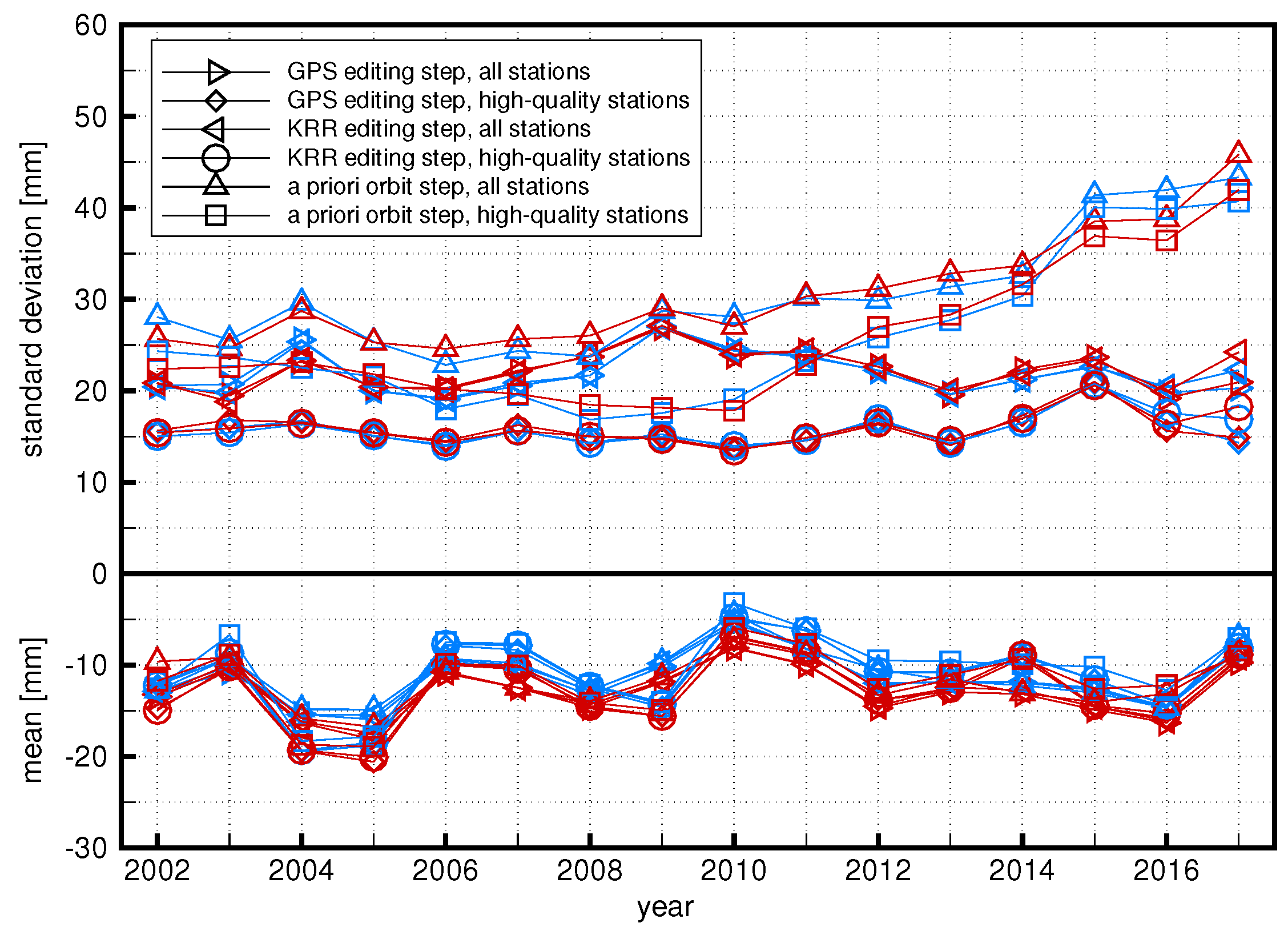
Another independent orbit validation during RL06 processing is routinely done by means of satellite laser ranging (SLR) observations from ground stations to the GRACE satellites, provided by the International Laser Ranging Service (ILRS). Coarse outliers in the SLR observations are eliminated by a 20 cm threshold. Mean values and standard deviations of GRACE-A and -B SLR residuals per year are shown in
Figure 2 for all available stations and a subset of high-quality stations. The definition of such a subset has been outlined by Arnold et al. [
37] and the same 12 stations are used here for better comparability. These high-quality stations contribute between 50% and 75% of all available observations. It can be seen that the standard deviations are in the range of 20 mm to 25 mm for all stations and about 15 mm for the high-quality stations. For the year 2010, the standard deviations for GRACE-A are 24.5 mm and 13.7 mm, respectively, which agrees very well with values of 24.4 mm and 12.3 mm, respectively, reported in [
37]. As for the GPS residuals, the values are the same whether only GPS observations are used or KRR observations are added, and are also very similar for both GRACE satellites. Increased standard deviations, in particular for recent years, are observed for the a priori orbits which can be explained by the fact that these orbits are determined without a time-variable gravity background model and GPS observations are down-weighted. The mean values of GRACE-A and -B as are also very consistent, independent of the processing step or whether all or the high-quality stations are evaluated. They are mostly in the range of −10 mm to −15 mm which is relatively large. However, this is not necessarily due to the orbit quality, but may also be caused by incorrect values for the GPS phase center offset (PCO) of the GRACE GPS navigation antennas. For GFZ RL06, PCOs relative to the antenna reference point provided by Montenbruck et al. [
38] are used. A geometrical offset (distance between the satellites’ center of mass and the antenna reference point) of −444 mm is added–only for the z-component in the SRF–resulting in a total L3 PCO in z-direction of −391.7 mm. This value is approx. 22 mm larger than the corresponding value derived from the official GRACE L1B vector offset product for the GPS main antenna (VGN1B, see [
21]) which might at least partly explain the relatively large negative offsets reported here.
Overall, the quality of the GFZ GRACE RL06 orbits is satisfyingly well confirming that the processing changes relative to GFZ RL05a have been a step into the right direction.
3. Results
GFZ GRACE RL06 gravity field results are analyzed and discussed in comparison to GFZ’s RL05a GRACE time series in the following subsections. Most of the results shown are relative to a climatology model (individually derived for each time series) which has been estimated as follows: The dominating signal content of the time series is approximated by fitting a proper parameter model coefficient-wise to the monthly solutions. Here, eight parameters describing the constant and linear part as well as periodic sine and cosine amplitudes for annual, semi-annual and 161-days (GRACE aliasing period for the ocean tide S2) periods are used. Furthermore, the formal errors of the monthly SH coefficients are used as a priori information to weight each individual monthly coefficient when estimating the climatology. Months with short repeat cycles (i.e., solutions which were regularized in RL05a) as well as the seven “GRACE single ACC” solutions are excluded.
3.1. Formal and Empirical Errors
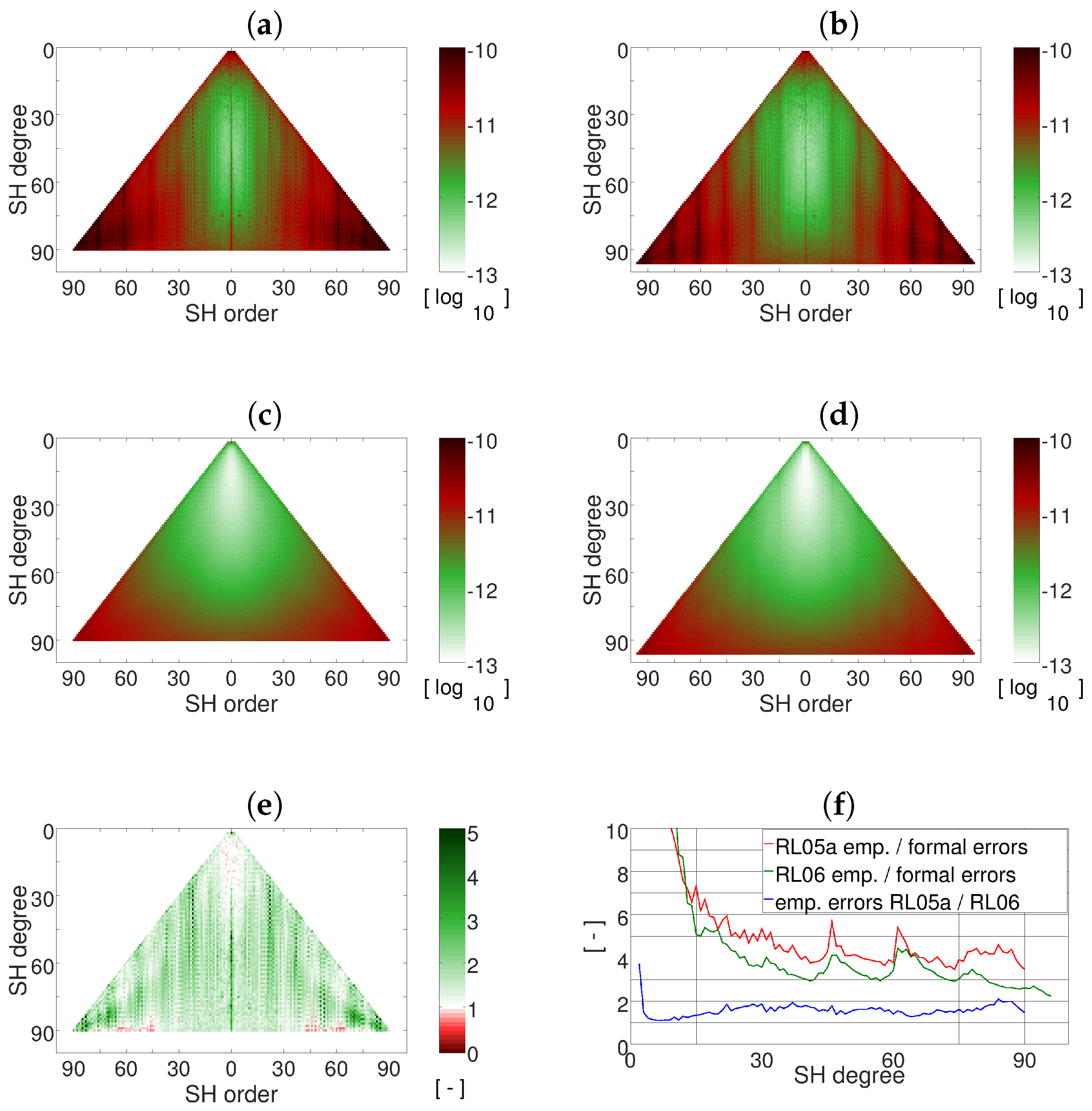
In this subsection formal and empirical errors of the GFZ RL06 time series are analyzed in the spectral domain and compared to GFZ RL05a. The formal errors are the standard deviations of the gravity field parameters estimated in the least-squares adjustment process, i.e., the square root of the diagonal of the gravity field parameter part of the variance-covariance matrices. In principle, these errors should give a good indication of the real errors of the estimated parameters. However, as variance-covariance information of all the input data is insufficiently (observations) or not all (background models) applied, the formal errors are typically too optimistic.
Another quantification of the errors of such a gravity field time series are empirically derived values. Here, residuals regarding the climatology described above are defined as empirical errors of the time series.
Figure 3 shows the RMS over the whole time series of the empirical and formal errors for RL05a and RL06. The main differences between empirical and formal errors can be seen in the very low SH degrees and around so-called resonance orders. Due to residual signals in the very low degrees, which are not covered by the eight parameters, the empirical errors show much higher values than the formal ones here. Around the resonance orders, which are integer multiples of approximately 15, it is well known that GRACE errors are larger due to systematic effects from temporal aliasing caused by background model errors. This effect is not very well represented in the formal errors.
Compared to RL05a (
Figure 3a,c),
Figure 3b,d reveal smaller empirical errors and more realistic formal errors for RL06. This becomes even more clear when looking at the ratio of the empirical error RMS values between RL05a and RL06 (
Figure 3e) which is > 1 for nearly all coefficients and also when plotted as amplitudes per SH degree (
Figure 3f). Also, the degree amplitudes of the ratio between empirical and formal errors indicate that the GFZ RL06 formal errors are more realistic as smaller variations than for GFZ RL05a are visible and the curve is closer to the value of one.
3.2. Degree Amplitudes
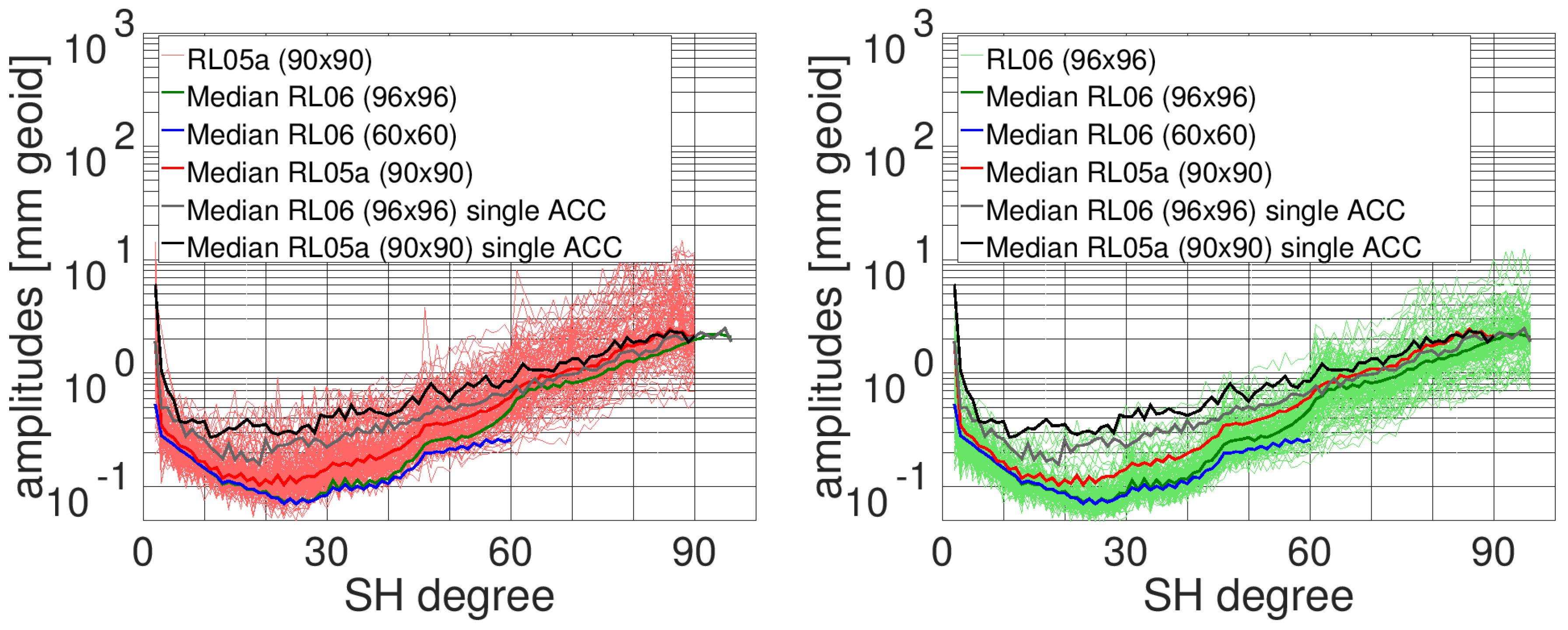
Difference degree amplitudes relative to climatology are shown in
Figure 4. The spread of monthly degree amplitudes is less for RL06 than for RL05a which illustrates that RL06 is a more homogeneous time series. Significant differences between the RL05a and RL06 median degree amplitudes are already visible at approx. SH degree 15, and almost all monthly RL06 degree amplitude curves are well below the median RL05a curve (or vice versa) for medium and high degrees indicating a notably improved signal-to-noise ratio for RL06. When only looking at the “GRACE single ACC” period, large improvements from RL05a to RL06 are achieved according to the corresponding median degree amplitudes. These improvements are not only present for medium and high degrees, but also for the very low degrees. However, the quality of the “GRACE single ACC” solutions is still significantly worse than for the rest of the GRACE mission also in case of RL06.
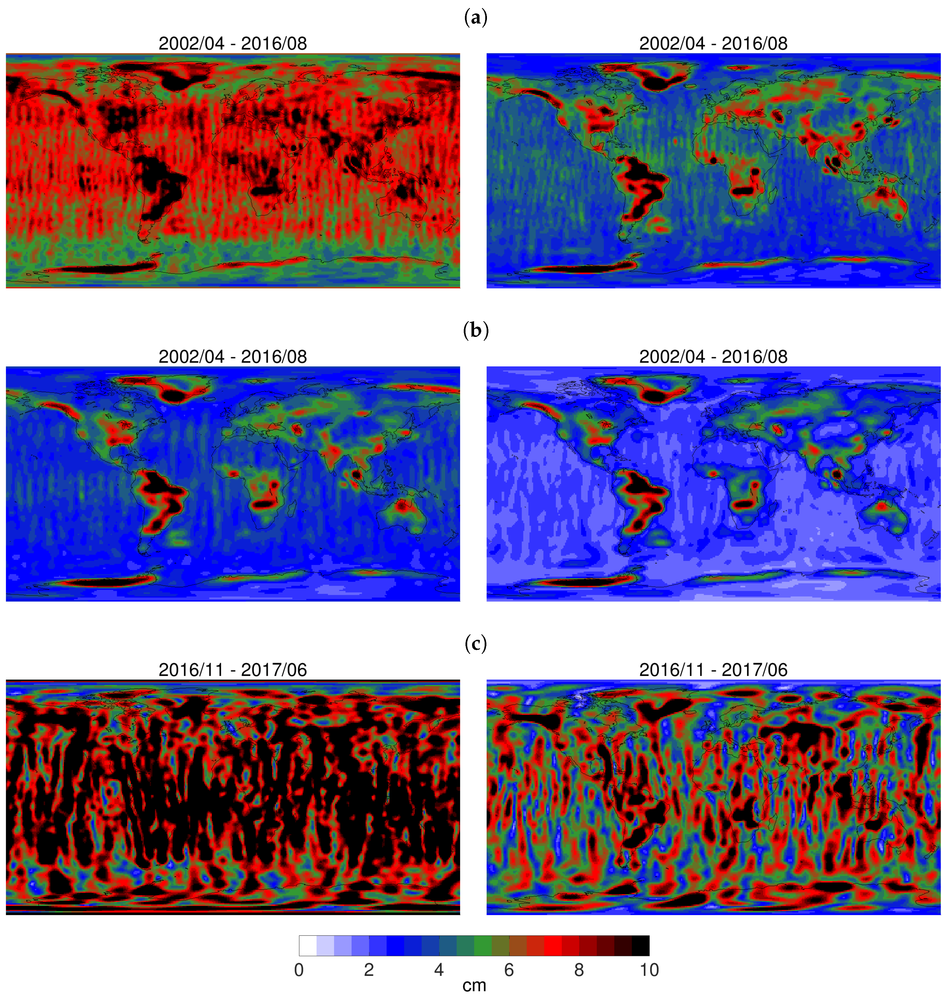
3.3. RMS of Residuals in the Spatial Domain
To assess the quality of the GFZ RL06 time series in the spatial domain, monthly residual SH coefficients relative to climatology are converted to gridded mass anomalies in terms of equivalent water height (EWH). To reduce the impact of spatially correlated noise, the solutions are de-correlated and smoothed by applying the non-isotropic DDK filter [
39]. Then, RMS values of the time series per grid point are calculated and shown in
Figure 5. For the period until August 2016, i.e., without the “GRACE single ACC” months, a clear reduction of RMS variability for RL06 has been achieved (
Figure 5a,b). Geophysical signals over continental areas, where they are much larger than over the oceans, are less superimposed by the typical GRACE striping pattern and thus better detectable. Variability over the oceans is generally expected to be rather small and is therefore often interpreted as upper error bound for monthly global GRACE gravity field models. Latitude-dependent weighted RMS (wRMS) values over the oceans decrease from 6.8 cm (RL05a) to 4.0 cm (RL06, 41% relative improvement) when DDK5 filtered, and from 3.4 cm (RL05a) to 2.1 cm (RL06, 38% relative improvement) when DDK3 filtered. For the “GRACE single ACC” period,
Figure 5c shows DDK3 filtered RMS variability to allow a direct comparison with the period before, but it becomes obvious that much stronger decorrelation and smoothing would be required here to extract geophysical signals. Nevertheless, the corresponding wRMS values over ocean decrease again significantly from 9.5 cm (RL05a) to 6.1 cm (RL06, 36% relative improvement).
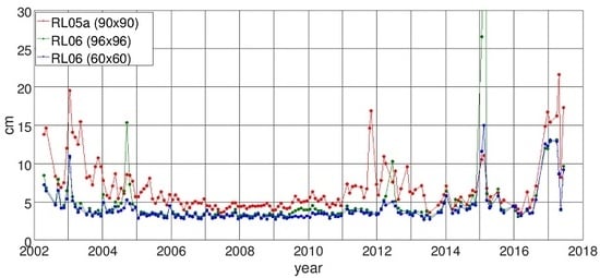
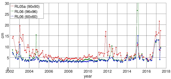
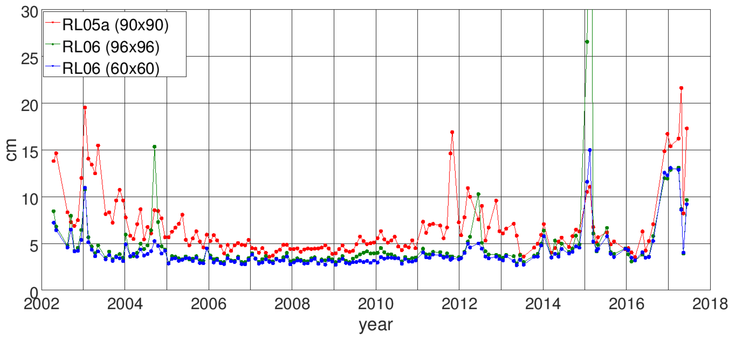
Monthly wRMS values over the oceans for the complete GRACE time series (DDK5 filtered) are shown in
Figure 6. Again, it becomes visible that GFZ RL06 is a clear improvement over RL05a in terms of noise reduction and homogeneity. Some months where RL06, particularly for the 96 × 96 time series, exhibits larger wRMS values than RL05a can be attributed to short period repeat orbit cycles (the most harmful repeat orbits during the GRACE mission are: 61/4 around September 2004, 46/3 around May 2012, 77/5 around December 2013, 31/2 around February 2015). RL05a solutions for these months were regularized which is not the case anymore for RL06 as the additionally provided RL06 60 × 60 time series, which is less sensitive to these short period repeat orbits, might be analyzed instead. Apart from the repeat cycles just mentioned before, the wRMS values of the RL06 96 × 96 and 60 × 60 time series are mostly almost identical. Periods where these values are notably larger are again related to less harmful repeat cycles such as the long-lasting 107/7 repeat orbit around December 2009. Finally, also
Figure 6 shows that the “GRACE single ACC” months are of much less quality than the rest of the time series. At least, the RL06 solution for May 2017 is now of comparable quality (it must be noted that for this solution GRACE-B ACC data is actually available and used).
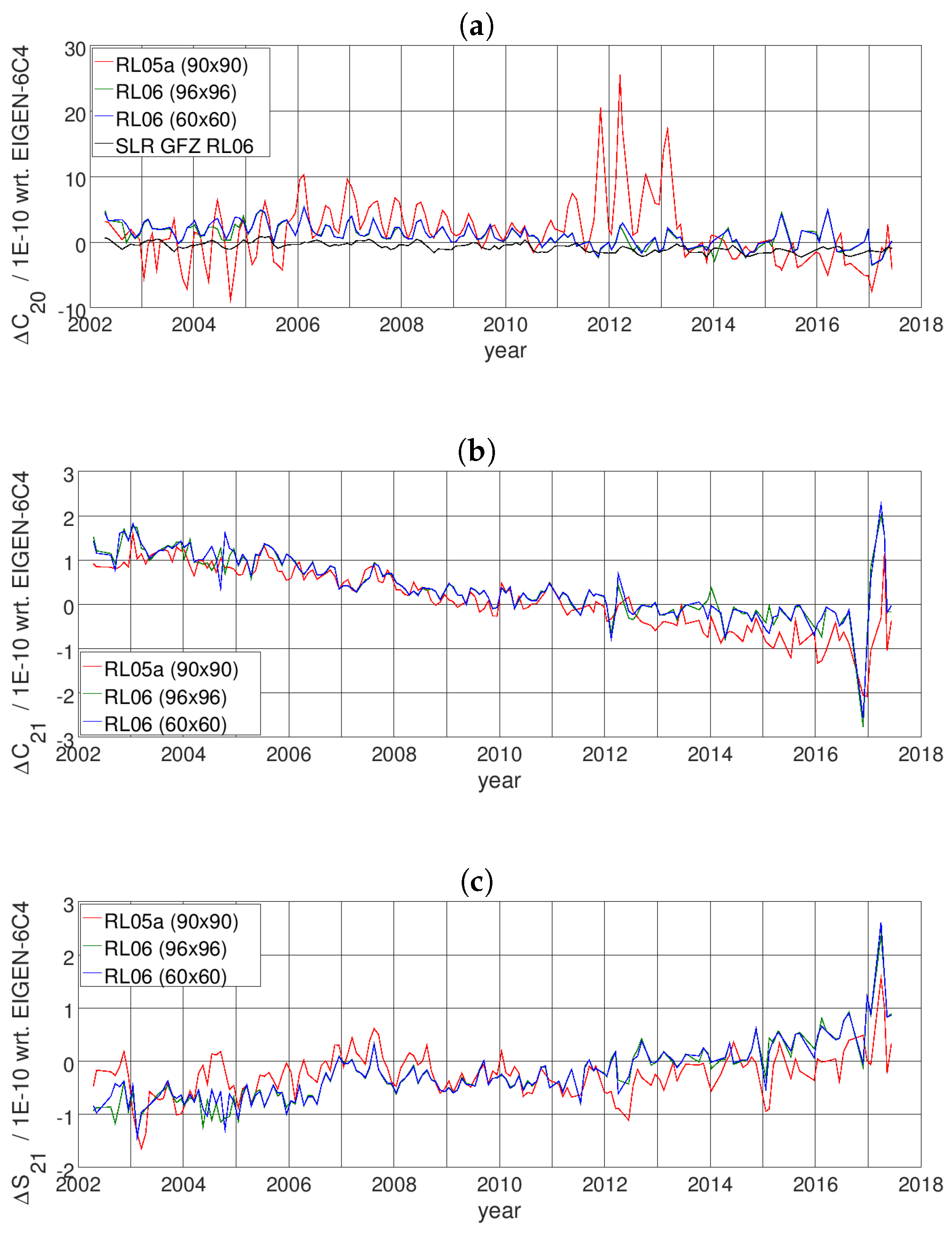
3.4. Low Degree Harmonics
In this subsection, time series of selected low degree SH coefficients are analyzed, starting with C
. This coefficient is known to be poorly estimated from GRACE (see, e.g., [
40]), and it is common practice to replace it, e.g., with estimates derived from SLR observations to geodetic satellites. Despite the fact that the GFZ GRACE RL06 C
values have significantly improved compared to GFZ RL05a (
Figure 7a), a replacement of C
is still recommended for RL06 before using the time series for geophysical interpretation. Available SLR-based replacement time series which are consistent with RL06 standards are, e.g., GRACE Technical Note TN-11 generated by CSR [
41], or a similar time series provided by GFZ [
42] which is also shown in
Figure 7a.
Two other coefficients requiring special attention are C
and S
. When analyzing surface mass variations from the GRACE SDS RL05 time series, Wahr et al. [
43] recommended corrections to these coefficients to account for effects of the applied mean pole model. Since all three SDS RL06 time series including GFZ RL06 are processed based on a linear mean pole model which is conform to the updated IERS2010 mean pole convention (
http://iers-conventions.obspm.fr/chapter7.php), this recommendation is not applicable anymore to these reprocessed time series. Looking at the GFZ RL06 C
time series in comparison to GFZ RL05a (
Figure 7b), however, one can see an anomalous behavior during the “GRACE single ACC” period. Although already the RL05a time series shows larger amplitudes in that period, this is even more pronounced in RL06. A similar behavior is visible also for S
(
Figure 7c). The reason for these anomalies in C
and S
is not yet fully understood and subject to further investigation. As it is clearly correlated with the use of ACC data transplant, a possible explanation would be that it is due to inaccurate modeling of surface forces, potentially in conjunction with an inappropriate parametrization. First experiments at GFZ combining GRACE and SLR on NEQ level have revealed promising results and might lead to a replacement time series, similar to C
, to overcome these deficiencies in the near future. It should be mentioned here that a GRACE+SLR combination would not be a novelty as, e.g., the GRACE solutions provided by the CNES/GRGS group are in fact already based on a combination with SLR [
15].
5. Conclusions
GFZ has reprocessed an improved monthly gravity field time series for the complete GRACE mission consisting of 163 gravity field models (Level-2 products) in the period from April 2002 through June 2017. This GFZ GRACE RL06 time series incorporates a reprocessed in-house GPS constellation (orbits and clocks), reprocessed Level-1B K-band ranging, star camera and accelerometer (ACC) transplant observations (L1B RL03 dataset provided by JPL), updated background models for tidal (FES2014) and non-tidal (AOD1B RL06) mass variations, and a considerably modified processing strategy including a different parametrization with (for most months) even less parameters compared to the precursor GFZ RL05a. Key features of the new RL06 processing strategy are a strict separation of GPS and K-band data editing, manual instead of automated sigma-based K-band data editing, and omittance of a time-variable gravity background model during the gravity field estimation step. Main differences in RL06 parametrization compared to RL05a are consistently estimated parameters throughout all processing steps, less ACC parameters (biases and scale factors), and –exclusively for the last months where ACC transplant data has to be used for GRACE-B (“GRACE single ACC” period)–the estimation of a fully populated ACC scale factor matrix. Independent validation by satellite laser ranging (SLR) observations reveals a satisfying quality of the GRACE orbits prior to gravity field adjustment with standard deviations of SLR residuals < 20 mm for selected high-quality stations.
With the new GFZ RL06 time series significant improvements have been achieved: The noise is considerably reduced and, consequently, geophysical signals are better detectable and can be analyzed at smaller spatial scales. Relative improvements over GFZ RL05a in terms of residual RMS variability are about 40% for both DDK3 and DDK5 filtered solutions. Furthermore, the complete time series is more homogeneous. Although the GFZ RL06 formal errors are still too optimistic for most of the gravity field coefficients, they exhibit a more realistic behavior, and also empirical errors in terms of residuals relative to a climatology model are smaller than for GFZ RL05a. The quality of the gravity fields within the “GRACE single ACC” period is clearly worse compared to the rest of the time series, but relative to RL05a, the RL06 solutions are also significantly improved here. Special attention needs to be paid to the C
and S
coefficients showing unrealistic amplitudes during that period. A combined GRACE+SLR replacement time series for these coefficients might help to mitigate this issue, as first investigations at GFZ have indicated. Regarding the C
coefficient, known to be poorly estimated from GRACE, it is still advised to replace the values by external time series, e.g., derived from SLR. Such a time series that is consistently processed with GRACE RL06 standards, is also provided by GFZ [
42].
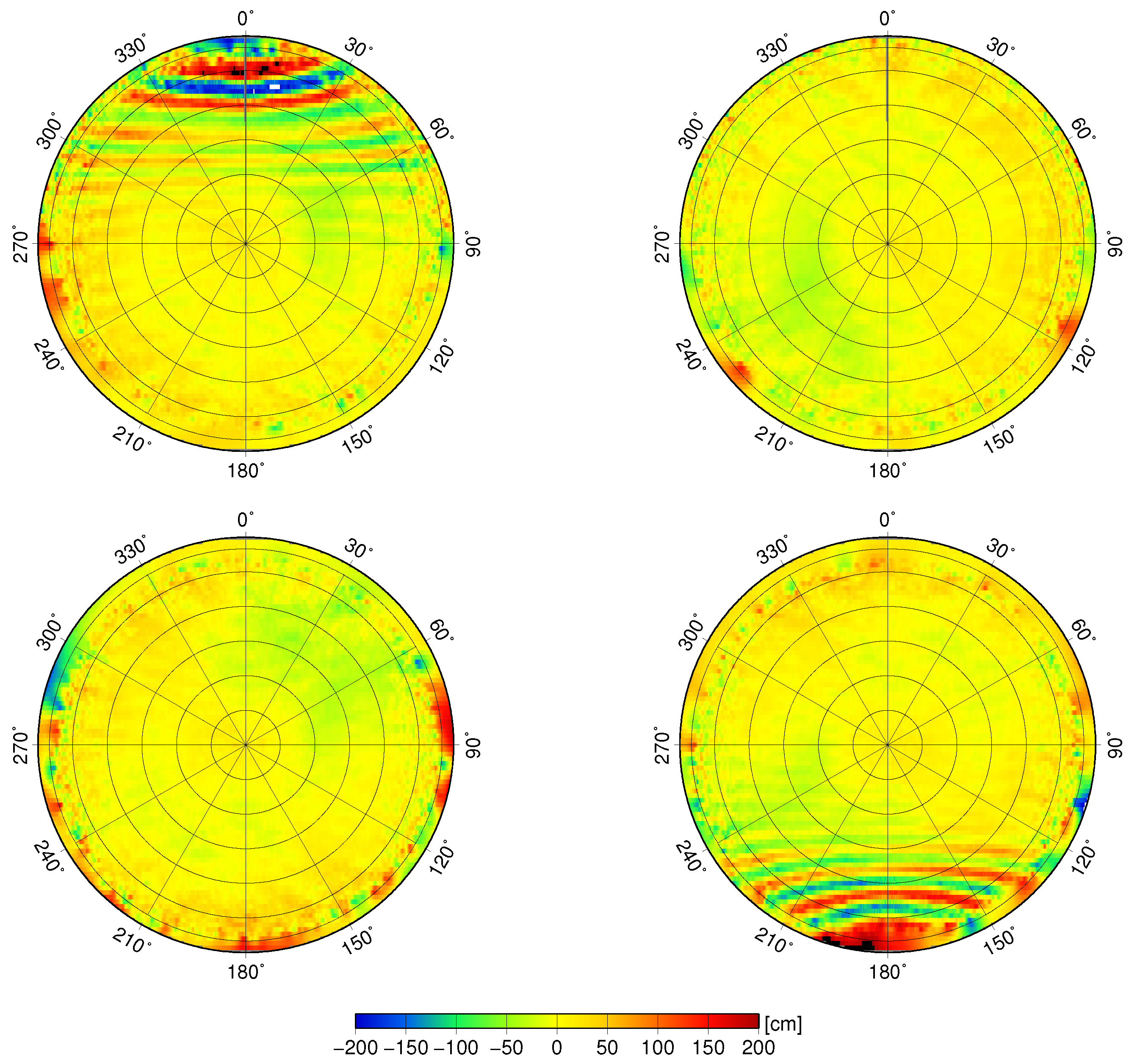
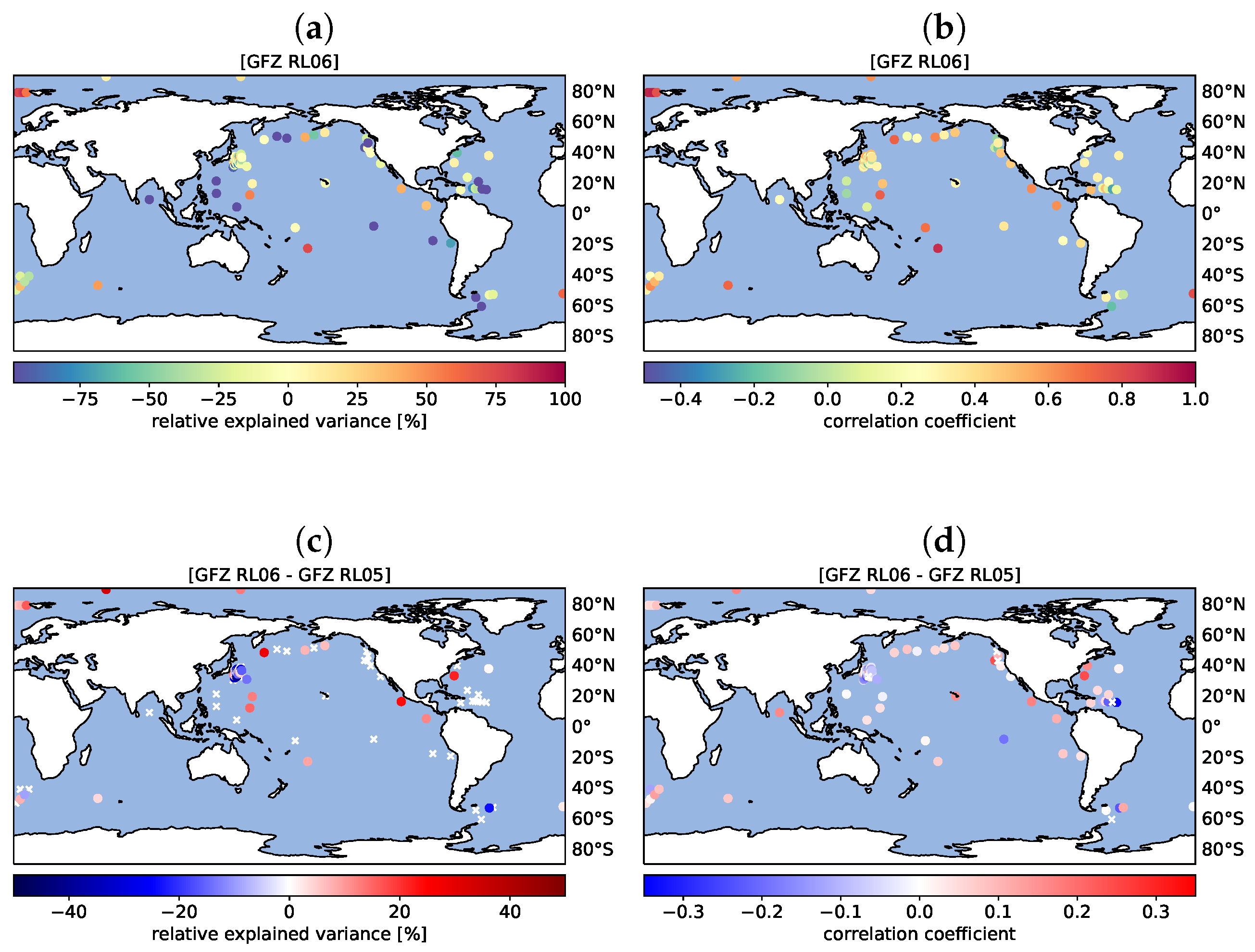
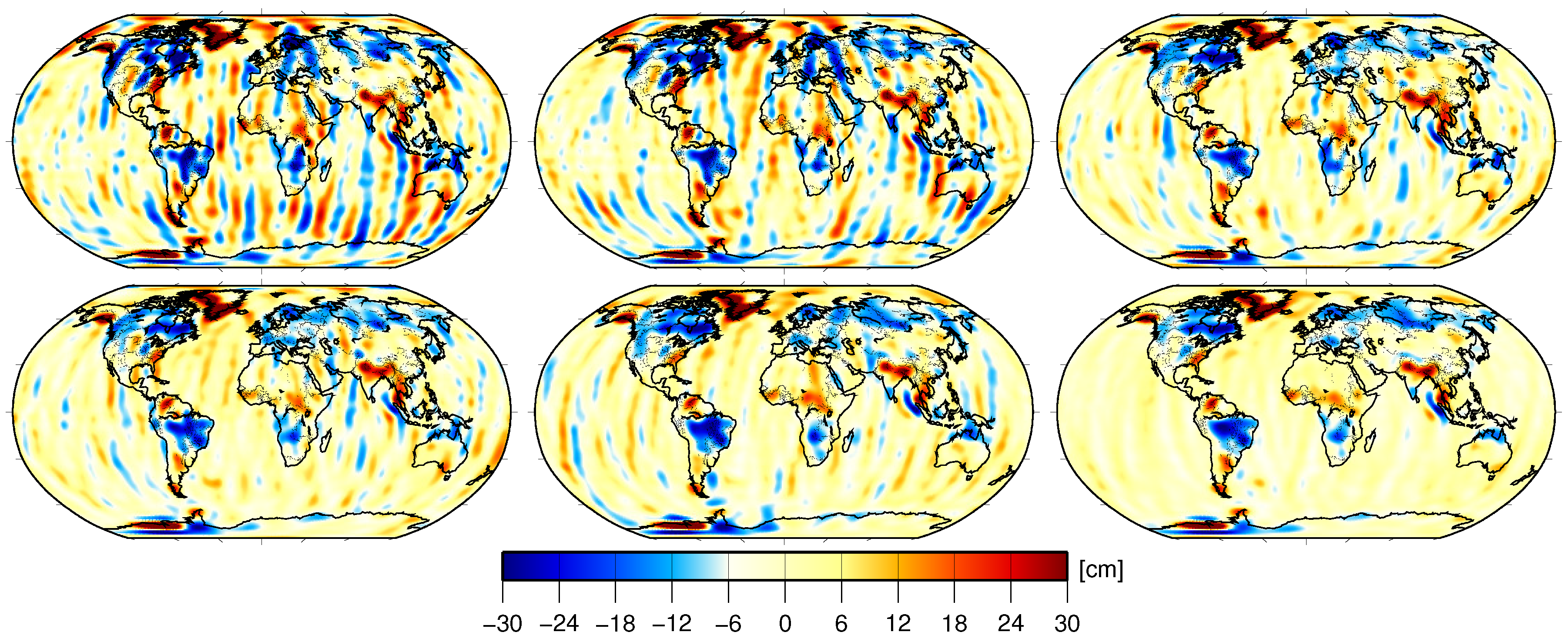
External validation by means of comparison with in situ ocean bottom pressure observations as well as orbit tests with the GOCE satellite confirm that improvements have been achieved with GFZ RL06 over RL05a, enabling thus a better understanding of phenomena in the Earth system related to climate change. To put the relative improvement from RL05a to RL06 in context with the relative improvements between all GFZ GRACE releases since RL01,
Figure 9 shows gravity field anomalies for all previous GFZ GRACE releases exemplarily for the month August 2003. The corresponding relative improvements in terms of wRMS over ocean are as follows: RL01 to RL02: 14%, RL02 to RL03: 24%, RL03 to RL04: 4%, RL04 to RL05a: 0%, RL05a to RL06: 41%. This is another clear indication of the remarkable improvements achieved with the GFZ RL06 reprocessing and also depicts that even after more than 15 years of the first instrument data release a substantial gain in the quality of monthly GRACE gravity field products is possible thanks to reprocessing efforts regarding Level-1 and Level-2 products, but also improved background models and enhanced processing strategies. Hence, reprocessing of a GRACE RL07 time series is already planned, for which a final release of Level-1 products will be available. Apart from using these new Level-1 data and possible background model updates, the specific focus at GFZ for RL07–or other likely upcoming releases–will be on the reported C
/S
issue, as well as on a further reduction of noise as achieved by other groups (see, e.g., [
14]). Whereas modification or fine tuning of the parametrization is always a promising option in view of improvements, in particular the application of an improved stochastic modeling of errors in observations and background models is envisaged.
A comparison between GFZ RL06 and recently published GRACE time series by other processing centers is not the purpose of this work; however, such comparisons were already done in several other studies: Göttl et al. [
56] report an increased consistency of the SDS (CSR, JPL, GFZ) RL06 and ITSG-Grace2018 solutions compared to the SDS RL05 and ITSG-Grace2016 solutions. Kvas et al. [
14] investigated the signal content of the SDS RL06 and ITSG-Grace2018 solutions by evaluating river basin averages and conclude that all four solutions exhibit the same signal content. Adhikari et al. [
57] calculated sea-level fingerprints using the SDS RL06 time series and find that differences between these three solutions are within 1-sigma uncertainties.
GFZ GRACE RL06 processing standards and background models are also used for the initial GFZ GRACE-FO Level-2 product release [
58]. Moreover, GFZ GRACE/GRACE-FO RL06 Level-2 products are the basis for GFZ’s web portal GravIS (Gravity Information Service,
http://gravis.gfz-potsdam.de), jointly developed with the Alfred-Wegener-Institut and TU Dresden, where dedicated Level-3 products for hydrological, oceanic and polar ice-sheet applications are visualized and offered for download. Finally, the GFZ GRACE RL06 time series contributes to the newly established International Combination Service for Time-variable Gravity Fields (COST-G), a product center of the International Gravity Field Service (IGFS).

 ,
, 


