Article

Estimating Peanut Leaf Chlorophyll Content with Dorsiventral Leaf Adjusted Indices: Minimizing the Impact of Spectral Differences between Adaxial and Abaxial Leaf Surfaces

1
Key Laboratory of Geographical Processes and Ecological Security in Changbai Mountains, Ministry of Education, School of Geographical Sciences, Northeast Normal University, Changchun 130024, China
2
Faculty of Science, University of Technology Sydney, Sydney, NSW 2007, Australia
3
School of Geography and Environmental Science, University of Southampton, Highfield, Southampton, SO17 1BJ, UK
4
Agronomy College, Shenyang Agricultural University, Shenyang 110866, China
5
Ministry of Agriculture Key Laboratory of Plant Nutrition and Fertilizer, Institute of Agricultural Resources and Regional Planning, Chinese Academy of Agricultural Sciences (CAAS), Beijing 100081, China
*
Author to whom correspondence should be addressed.
These authors contributed equally to this work.
Remote Sens. 2019, 11(18), 2148; https://doi.org/10.3390/rs11182148
Submission received: 16 August 2019 / Revised: 7 September 2019 / Accepted: 11 September 2019 / Published: 15 September 2019
(This article belongs to the Special Issue Hyperspectral Remote Sensing of Agriculture and Vegetation)

Abstract

:
Relatively little research has assessed the impact of spectral differences among dorsiventral leaves caused by leaf structure on leaf chlorophyll content (LCC) retrieval. Based on reflectance measured from peanut adaxial and abaxial leaves and LCC measurements, this study proposed a dorsiventral leaf adjusted ratio index (DLARI) to adjust dorsiventral leaf structure and improve LCC retrieval accuracy. Moreover, the modified Datt (MDATT) index, which was insensitive to leaves structure, was optimized for peanut plants. All possible wavelength combinations for the DLARI and MDATT formulae were evaluated. When reflectance from both sides were considered, the optimal combination for the MDATT formula was ( R 723 R 738 ) / ( R 723 R 722 ) with a cross-validation R2cv of 0.91 and RMSEcv of 3.53 μg/cm2. The DLARI formula provided the best performing indices, which were ( R 735 R 753 ) / ( R 715 R 819 ) for estimating LCC from the adaxial surface (R2cv = 0.96, RMSEcv = 2.37 μg/cm2) and ( R 732 R 754 ) / ( R 724 R 773 ) for estimating LCC from reflectance of both sides (R2cv = 0.94, RMSEcv = 2.81 μg/cm2). A comparison with published vegetation indices demonstrated that the published indices yielded reliable estimates of LCC from the adaxial surface but performed worse than DLARIs when both leaf sides were considered. This paper concludes that the DLARI is the most promising approach to estimate peanut LCC.

Graphical Abstract

1. Introduction

Peanut (Arachishypogaea L.) is one of the major food legumes as well as oilseed crops being grown in 118 countries (or regions) around the world on about 28 million ha of land [1], and offers multiple benefits to meet human nutritional needs as well as being an important resource in the context of food security and hunger issues [2]. Leaf chlorophyll content (LCC) is an important indicator of plant photosynthesis [3], nutritional state [4], and stress [5]. Determination of LCC is crucial for crop management and precision agriculture practices [6].
Spectral vegetation indices, which are defined with the objective of enhancing spectral sensitivity to vegetation properties, have long been popular for estimating vegetation’s biophysical and biochemical variables [7,8]. Decades of research have gone into determining wavelength regions sensitive to LCC in order to develop indices to maximize the accuracy of retrieval for different types of plants [9,10,11]. Datt [12] developed a three-band index for retrieval of LCC in higher plants based on the different response of reflectance at 710 nm and 850 nm to LCC. Sims and Gamon [13] analyzed nearly 400 leaf samples from 53 species and found that the mSR705 (simple ratio) and mND705 (normalized difference) were relatively insensitive to species and leaf structural variation. Gitelson et al. [14] proposed an index (RnirRred-edge − 1), which is an effective LCC predictor for maple, chestnut, wild vine, and beech leaves.
The pinnate leaves of peanut are highly sensitive to excess solar radiation and drought stress [15]. Field observations show that under strong solar irradiance, peanut easily turns the abaxial surface of leaves upwards. As a result, the spectral reflectance recorded by satellites or spectroradiometers may represent a mixture of the adaxial and abaxial surfaces in different proportions. The differences in optical properties of dorsiventral leaves due to the structural difference among the two sides have been well documented [16,17]. Baránková et al. [18] found that light incident from the adaxial side is more effectively absorbed than light incident from the abaxial side of green tobacco leaves. Lu and Lu [19] reported the lower reflectance of the adaxial white poplar surfaces compared to the abaxial faces in the 400–700 nm spectrum but reported an inversion of this effect in the near infrared wavelengths (700–1000 nm).
Leaf optical properties are a vital factor in determining the sensitivity of vegetation indices to LCC [13]. However, to the best of our knowledge, few studies have considered the influence of abaxial leaf reflectance on the retrieval of biochemistry and structure parameters. In one of the few studies carried out, Lu et al. [20] extended the wavelengths in the Datt’s index to incorporate spectral reflectance from 400 nm to 1000 nm. They found that the modified Datt’s index (MDATT) efficiently reduced the effects of bifacial leaf structure and improved the retrieval of white poplar and Chinese elm LCC. However, several characteristics of peanut leaves, such as leaf hair, wax, palisade, and spongy tissues, substantially differ from woody plants. Thus, the applicability of the MDATT to peanut LCC retrieval requires further investigation. In addition, the structural effects were mostly removed by MDATT but partially remained [21].
Theoretically, multiple-band indices can incorporate a larger amount of information and have the potential to improve retrieval accuracy [22,23,24,25,26]. For example, the mSR705 and mND705, which were developed by adding a band (R445) to the exiting two-band indices SR705 and ND705, effectively improved sensitivity to LCC [13]. Similarly, three-band indices such as the MERIS terrestrial chlorophyll index (MTCI) [22] and OLCI terrestrial chlorophyll index (OTCI) has been successfully used to retrieve chlorophyll content at the canopy scale (i.e., chlorophyll content) [27,28,29]. To date, very few studies have been conducted to assess the potential of vegetation indices based on four or more bands for improving LCC retrieval accuracy.
To address these gaps, this paper focuses on the development and optimization of new and existing indices that are insensitive to spectral differences among two sides of peanut leaves. The objectives of this work were to (1) analyze spectral differences in the adaxial and abaxial surfaces of peanut leaves; (2) identify the optimal wavelengths of the MDATT for estimating peanut LCC; (3) develop a novel index based on a four-band combination to reduce spectral differences in dorsiventral leaves for improving LCC retrieval; (4) compare the performance of the indices developed in this study with those widely used in the literature.

2. Materials and Methods

2.1. Data Collection

Ground data collection was carried out over a farmland area in Changchun, Jilin Province, China (44°42′27″N, 124°53′08″E), which is located in the temperate and monsoon climate zone with a typical continental climate. The field size was approximately 2 ha. During the peanut growing season in 2018, three field campaigns were conducted on 27 July (acicula forming stage), 19 August (bearing pod stage), and 19 September (maturity stage) to collect peanut leaves, respectively. In each campaign, 20 plots were randomly selected. One or two plants were selected at each plot, and leaves that were fully expanded, homogenous in color, and showing no visible signs of damage were detached from the top to the bottom of the canopy [30]. They were, immediately packed and sealed into plastic bags and placed inside a cooler (the interior temperature of the cooler was 0 °C) to avoid desiccation and decomposition of the chlorophyll by light. In each campaign, we collected 28 leaves. Thus, a total number of 84 leaves were used for spectral measurement and chlorophyll extraction. All the measurements, including the spectral measurements and chlorophyll extraction, were carried out within 4 h of leaf harvesting to minimize changes in chlorophyll content. Figure 1 illustrates the phenomenon of peanut leaves changing orientation under strong solar irradiance, making the view of the canopy a mixture of the adaxial and abaxial sides (Figure S1).
The reflectance of the adaxial and abaxial surfaces was measured using an ASD FieldSpec® 3 portable spectroradiometer (Analytical Spectral Devices, Boulder, CO, USA) and a contact probe, equipped with an internal halogen source and directly attached to the leaf surface using a leaf clip accessory. The spectrometer can collect data in the 350–2500 nm spectral region, with a sampling interval of 1.4 nm in the 350–1000 nm wavelength range and 2 nm in the 1000–2500 nm wavelength range. The average of 10 separate measurements from each sample was recorded. To reduce errors associated with variations in illumination geometry, the contact probe was pressed to the leaf surface, which was illuminated by the internal light source, ensuring a consistent illumination geometry.
The LCC was determined from the same leaf samples used for reflectance measurements. Circular discs with a diameter of 6 mm were cut from each leaf. Leaf discs were extracted in the dark at room temperature for 24 h with 95% ethanol and shaken repeatedly to ensure chlorophyll was completely extracted, as indicated by the completely white appearance of the disc [31]. The absorbance of each extract was measured at 663 nm and 645 nm using a UV757CRT ultraviolet-visible spectrophotometer (Shanghai Precision Scientific Instruments Corporation, Shanghai, China). The LCC (μg/cm2) was then calculated according to the equations provided by Arnon [32]. In total, measurements of LCC and reflectance were collected for 84 leaves. The LCC values ranged from 21.50 to 70.55 μg/cm2 with a mean value of 40.78 μg/cm2 and a standard deviation of 11.68 μg/cm2.

2.2. Data Analysis

2.2.1. Construction of a Dorsiventral Leaf Adjusted Ratio Index

A semi-empirical leaf reflectance model was proposed by Baret et al. [33], and can be expressed as:
R = R s + S exp ( Σ k i C i )
where Rs is the reflectance of the leaf surface, S represents scattering effects of the leaf mesophyll structure, and ki and Ci are the extinction coefficient and chlorophyll concentration, respectively. Rs and S are thought to be the main factors introducing variability between adaxial and abaxial leaf reflectance, as they depend on the differences in the leaf surface and internal mesophyll structure Datt [12]. Based on this model and the principle that there is no absorption at 850 nm by any leaf pigment ( i . e . ,   Σ k i C i = 0 ), Datt [12] proposed an index of ( R 850 R 710 ) / ( R 850 R 680 ) . The index removed Rs and S. Lu et al. [21] extended the wavelengths in the Datt’s index to 400–1000 nm, which can also remove Rs and S. The formula of MDATT is:
MDATT = ( R λ 1 R λ 2 )   ( R λ 1 R λ 3 ) = exp ( K chl ( λ 1 ) C chl ) exp ( K chl ( λ 2 ) C chl ) exp ( K chl ( λ 1 ) C chl ) exp ( K chl ( λ 3 ) C chl )
where Cchl is the chlorophyll content and kchl(λ1), kchl(λ2), and kchl(λ3) are the specific absorption coefficients for Chl at wavelengths λ1, λ2, and λ3, respectively.
Using the MDATT as a basis, we constructed a dorsiventral leaf adjusted ratio index (DLARI) by substituting the R λ 1 term with an additional wavelength ( R λ 4 ) in the denominator:
DLARI = ( R λ 1 R λ 2 ) ( R λ 3 R λ 4 ) = exp ( K chl ( λ 1 ) C chl ) exp ( K chl ( λ 2 ) C chl ) exp ( K chl ( λ 3 ) C chl ) exp ( K chl ( λ 4 ) C chl )
Like the MDATT, the DLARI is also expected to suppress the effects of Rs and S. The efficiency of incorporating an additional band is evaluated in the following sections.

2.2.2. Published Vegetation Indices

The accuracy of LCC retrieval using the MDATT and DLARI indices was compared with that of 12 published vegetation indices that were originally proposed for chlorophyll content retrieval and have proven to be highly correlated with LCC [34]. The types of indices included single-band index (e.g., 1/R700), two-band indices (e.g., VOG1 = R740/R720), three-band indices (e.g., DATT = (R850 − R710)/(R850 − R680)), as well as four-band indices (e.g., VOG2 = (R734 − R747)/(R715 + R720)). The formulae of the indices are provided in Table 1. In addition, two MDATTs proposed by Lu et al. [21] were used to evaluate the optimal wavelengths in the MDATT for peanut LCC estimation. The first MDATT in Table 1 with wavelengths at 691 nm, 745 nm, and 736 nm was developed from the adaxial surface reflectance of woody plants, whilst the second MDATT with wavelengths at 721 nm, 744 nm, and 714 nm was based on a mixture of reflectance for both adaxial and abaxial surfaces.

2.2.3. Model Calibration and Validation

All possible band combinations based on the MDATT and DLARI derived from adaxial, abaxial, and the bifacial (i.e., including both adaxial and abaxial reflectance measurements) datasets were correlated with LCC, respectively. The waveband combinations with the highest coefficient of determination (R2) for each dataset were selected as the optimal indices and used to model LCC. Relationships between the measured LCC and indices were established using empirical regression analysis. The form of fitting functions (e.g., linear, exponential, logarithmic) relating the indices to LCC appeared to have a marginal impact when compared to the impact of band selection [24]. Therefore, we restricted the fitting method to ordinary least-squares linear regression.
The performance of the index-based models was evaluated using the R2 and root mean square error (RMSE) with respect to the biochemically measured LCC. In order to avoid dependence on a single random partitioning of the datasets and guarantee that all samples were used for both training and validation, a repeated 10 fold cross-validation was used to evaluate the performance of each index [40]. The dataset was split into 10 consecutive folds, and each fold was then used once for validation while the remaining 9 folds formed the training dataset. This process was repeated 50 times, and combined R2cv and RMSEcv values were calculated as the mean of those from each repetition.

3. Results

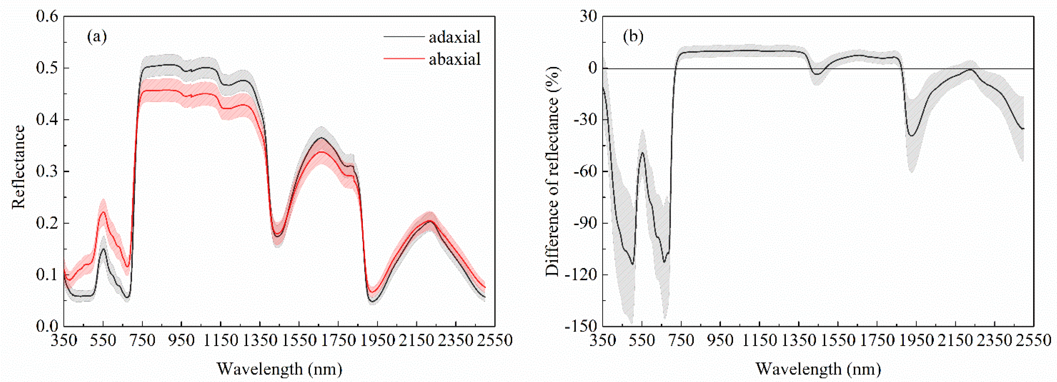
3.1. Spectral Differences Between Adaxial and Abaxial Surfaces

The mean spectral reflectance of the adaxial and abaxial surfaces is shown in Figure 2a. The reflectance of the adaxial surface was much lower than that of the abaxial surface in the visible region (400 to 690 nm). This is because light incident from the adaxial side was more effectively absorbed than light incident from the abaxial leaf side [18]. In contrast, the adaxial reflectance was higher than that of the abaxial surface between 750 and 1400 nm. This was partly because the palisade structure at the adaxial side of the leaf contributed higher reflected radiation than the spongy structure at the abaxial side [17]. Spectral differences among the two leaf surfaces were small in the red-edge region (690 to 750 nm), especially between 718 and 732 nm, where differences in reflectance were less than 5% (Figure 2b). Differences were also less substantial at wavelengths longer than 1400 nm. Variations in the internal structure of the adaxial and the abaxial surface also contributed to these differences (Figure 3). The adaxial surface (Figure 3a) was characterized by increased waxes than the abaxial surface (Figure 3b). Rayleigh scattering by waxes is known to contribute to the higher reflectance of the adaxial surface at NIR wavelengths [41].
The correlation between LCC and the reflectance of both surfaces are plotted in Figure 4. The reflectance of both surfaces in the blue region (400 to 500 nm) and the main chlorophyll absorption region near 680 nm demonstrated the least sensitivity to LCC. High sensitivity to LCC was observed at 570 nm and near 710 nm. The strongest correlation was at 710 nm (the correlation coefficient is −0.91) and 704 nm (the correlation coefficient is −0.85) for the adaxial and abaxial surfaces, respectively. The abaxial reflectance at wavelengths over 750 nm also demonstrated strong correlations. Overall, the correlations between LCC and abaxial reflectance were stronger than those between LCC and adaxial reflectance.

3.2. Relationships Between Optimal MDATT Indices and Peanut LCC

The relationship between LCC and the MDATT using band combinations ranging from 400 nm to 1000 nm was assessed for each dataset. The maximum R2 was determined by fixing λ2 and λ3 as single values and changing λ1 from 400 nm to 1000 nm. For the sake of concise display, only R2 values greater than 0.8 were considered and they are shown in Figure 5, where the x-axis represents λ3 and the y-axis λ2. From this figure, robust wavelength regions for each band of the MDATT can be identified. For the adaxial dataset, the most sensitive region (red color in Figure 5a) ranged from 700 nm to 800 nm for λ2, 400 nm to 800 nm for λ3, and 650 nm to 750 nm for λ1 (Figure 5d). The robust regions for the abaxial dataset were similar to those for the adaxial dataset (Figure 5b,e), but the most sensitive area (red color in Figure 5b) was reduced, and covered approximately 750 nm for λ2, 730 nm for λ3, and 690–750 nm for λ1. For the bifacial dataset (Figure 5c,e), the sensitive wavelength regions were further reduced. The R2 values greater than 0.88 were demonstrated when λ2 and λ3 were between 700 nm to 750 nm and λ1 was between 660 nm and 710 nm.
According to the principle of selecting indices demonstrating the highest R2 values, three optimal MDATT indices for each dataset were determined and are presented in Table 2. The wavelengths λ1, λ2, and λ3 of the best performing MDATT index for all three datasets were concentrated in the region of 701 to 747 nm. For the adaxial surface, the index incorporating reflectance values at 701 nm, 742 nm, and 740 nm demonstrated an R2 of 0.95, whilst for the abaxial dataset, the best index incorporated reflectance values at 718 nm, 747 nm, and 720 nm (R2 = 0.94). In the case of the bifacial dataset, the best index incorporated reflectance values at 723 nm, 738 nm, and 722 nm, reaching an R2 of 0.91. The optimal indices for the adaxial and abaxial surfaces employed at least one wavelength that was highly correlated to LCC (r < −0.60), i.e., 701 nm, 718 nm, and 720 nm (Figure 4). The reflectance values at 722 nm and 723 nm, which were used by the optimal index for the bifacial dataset, demonstrated the minimum differences between adaxial and abaxial surfaces (Figure 2b).
The linear models established using the MDATT indices are shown in Figure 6. They were randomly selected from one of the 50 training datasets used in the repeated 10 fold cross-validation. The results indicated that for the adaxial surface, the index ( R 701 R 742 ) / ( R 701 R 740 ) achieved the highest retrieval accuracy (R2cv = 0.95, RMSEcv = 2.52) (Figure 6a,d), followed by the index ( R 718 R 747 ) / ( R 718 R 720 ) for the abaxial surface (R2cv = 0.94, RMSEcv = 2.69) (Figure 6b,e). Both performed better than the index ( R 723 R 738 ) / ( R 723 R 722 ) for the bifacial dataset (R2cv = 0.91, RMSEcv = 3.53) (Figure 5c,f). The observed and predicted values fell close to the 1:1 line, indicating that the optimized MDATT indices were stable predictors of LCC. The optimal index for the bifacial dataset demonstrated a lower correlation with LCC and was not as accurate an LCC predicator as the other two indices.
Differences in adaxial and abaxial reflectance properties resulted in different MDATT indices and associated retrieval accuracies. The reliability of applying the optimal index for the adaxial surface to estimate LCC from bifacial reflectance measurements was investigated (Table 3). It showed that compared to the bifacial MDATT, applying the adaxial MDATT to estimate LCC from bifacial reflectance produced considerable errors (R2cv = 0.87, RMSEcv = 4.14). In light of the errors, it was necessary to consider the influence of spectral differences between adaxial and abaxial sides when estimating LCC from reflectance mixed by the two sides.

3.3. Relationships Between DLARI and Peanut LCC

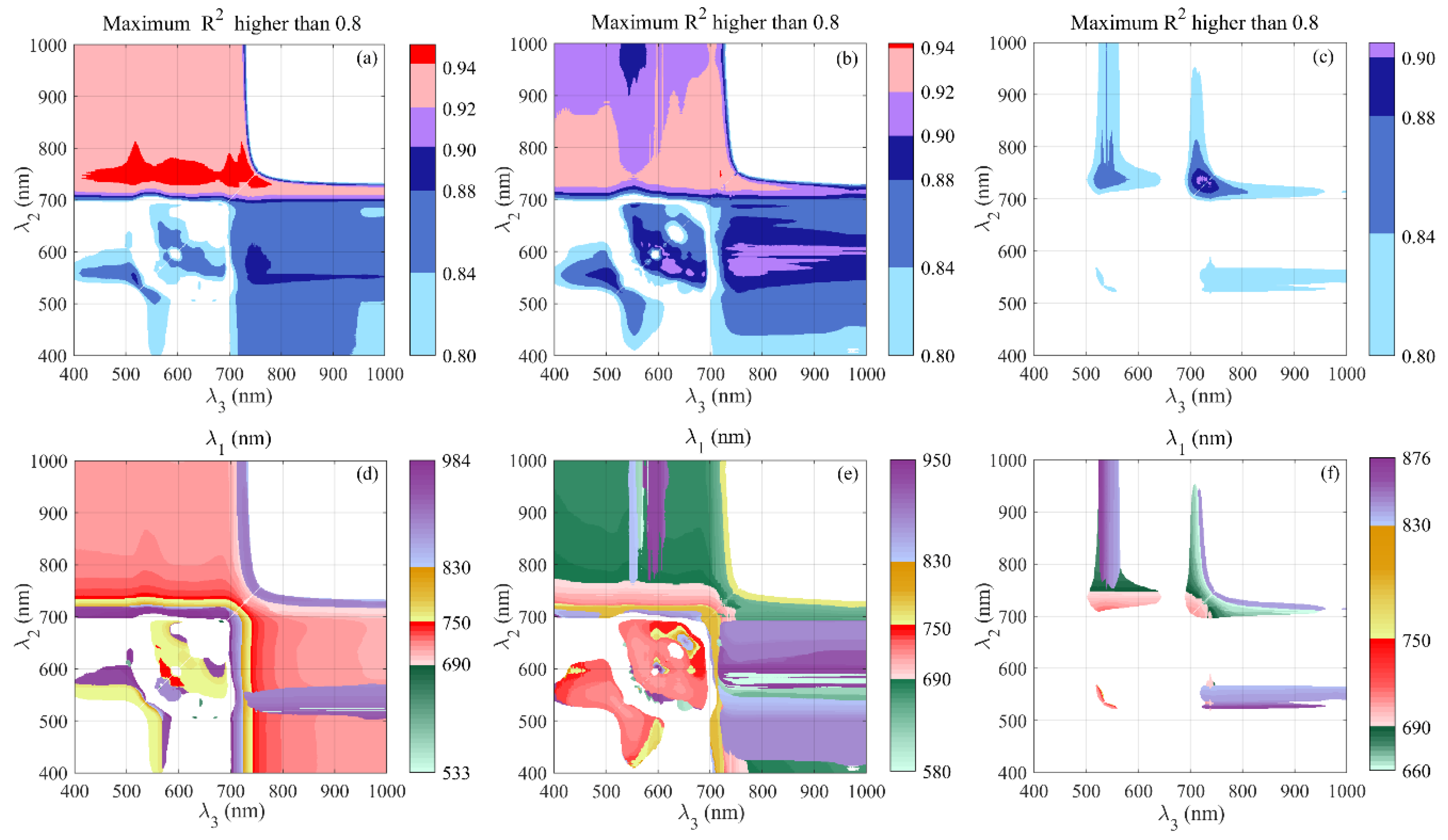
3.3.1. Performance of DLARIs Incorporating Wavelengths Between 660 and 750 nm

Because the most robust wavelength region was between 660 nm and 750 nm in the case of the MDATT, all possible DLARI combinations formed by Equation (3) using wavelengths from 660 nm to 750 nm were calculated. According to the principle of selecting the index that demonstrated the highest R2, optimal DLARIs were established for each dataset (Table 4). The results demonstrated that the wavelengths used in the DLARIs were similar to those used in the MDATTs (Table 2). When compared with the MDATTs for the adaxial surface, the DLARI did not improve retrieval accuracy (RMSEcv = 2.53), the DLARI for the abaxial surface demonstrated a marginal advantage over the abaxial MDATT (RMSEcv = 2.62). In the case of the bifacial dataset, the DLARI achieved some improvement over the bifacial MDATT (RMSEcv = 3.34).

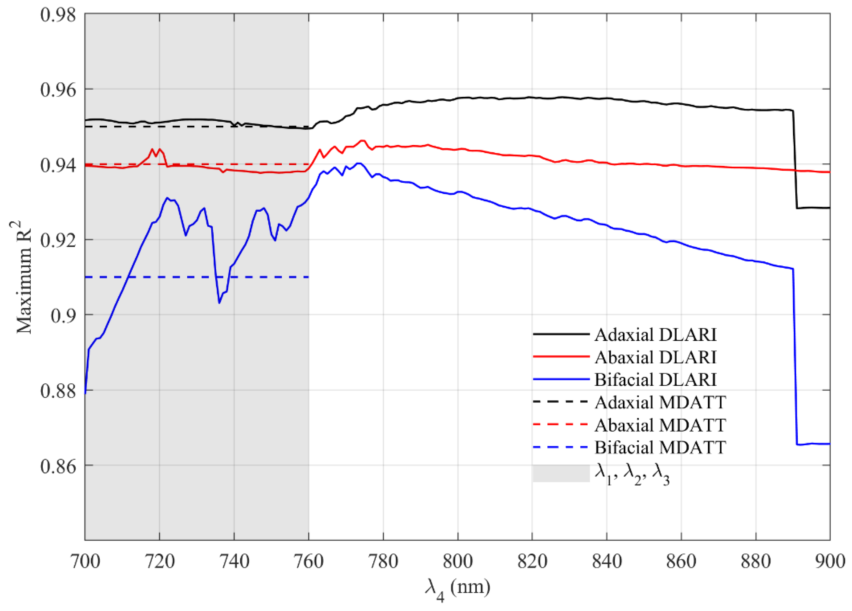
3.3.2. Performance of DLARIs Incorporating Wavelengths Over 750 nm

In the DLARIs for the bifacial dataset, the wavelength selected for λ4 was at the limit of the considered region (i.e., 750 nm), indicating that relevant information might be contained at longer wavelengths. When evaluated, DLARIs incorporating longer wavelengths (around 820 nm) achieved higher retrieval accuracies than those described in Section 3.3.1. (Table 5). It showed that for the three datasets, the optimal wavelengths of λ1 and λ3 moved to approximately 730 nm and 720 nm, where the differences in adaxial and abaxial reflectance were less than 5% (Figure 2). The optimal location of λ2 moved to the red-edge shoulder, which means less sensitivity to leaf structure [42], while the optimal location of λ4 moved to the NIR, where there is less absorption by leaf pigments [12]. The new adaxial DLARI and abaxial DLARI demonstrated advantages over the DLARIs derived from reflectance over 660 and 750 nm (RMSEcv = 2.37; RMSEcv = 2.58). The new bifacial DLARI not only substantially improved the retrieval accuracy (RMSEcv = 2.81), but also enhanced its sensitivity to LCC (R2cv = 0.94).
Relationships between LCC and the optimal DLARIs established are shown in Figure 7, as are scatter plots of the associated retrievals and observed values. For the adaxial and the abaxial datasets (Figure 7a,b,d,e), the indices ( R 735 R 753 ) / ( R 715 R 819 ) and ( R 731 R 755 ) / ( R 722 R 774 ) attained higher retrieval accuracies (R2cv = 0.96, RMSEcv = 2.37; R2cv = 0.95, RMSEcv = 2.58) than the MDATT indices (R2cv = 0.95, RMSEcv = 2.52; R2cv = 0.94, RMSEcv = 2.69). For the bifacial dataset (Figure 7e–f), the index ( R 732 R 754 ) / ( R 724 R 773 ) achieved an R2cv of 0.94 and RMSEcv of 2.81, demonstrating a substantial advantage over the bifacial MDATT index (R2cv = 0.91, RMSEcv = 3.53) and the DLARI derived using wavelengths shorter than 750 nm. The results revealed that the DLARIs incorporating longer wavelengths efficiently improved LCC estimation accuracy, whether for the adaxial, abaxial or bifacial datasets.

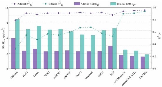
3.4. Comparing Developed Indices with Those of Previous Studies

The performance of the published vegetation indices for LCC retrieval using adaxial and bifacial reflectance measurements is shown in Figure 8, as is the performance of the indices developed in this study. The published indices, which ranged from single- to four-band formulae, produced reliable retrievals of LCC when applied to adaxial reflectance measurements. In general, the three-band indices performed better than the two-band indices and the two-band indices performed better than Gitelson’s index. The best performing indices were MTCI, DATT, and Maccioni followed by the four-band index VOG2. The red edge position index performed worse than all the three-band indices. However, when applied to the bifacial dataset, much lower R2cv and higher RMSEcv values were obtained. The VOG1, MTCI, mSR705, mND705, and VOG2 indices yielded RMSEcv values of approximately 3.5 from the adaxial dataset, while the RMSEcv values increased to 7.5 when applied to the bifacial dataset. Although the MTCI, mSR705, Maccioni, and DATT share the same format, the Maccioni and DATT indices (which employ two of the same wavelengths) performed better on the bifacial dataset. This was possibly because one of the bands used by Maccioni and Datt is located within the NIR region (780 nm and 850 nm), where there is little absorption by any leaf pigments ( Σ k i C i = 0) [12]. This partly reduces spectral differences caused by the different absorption properties of pigments at the adaxial and abaxial surfaces.
Among the published indices, Lu’s MDATTs, which uses different wavelengths for the adaxial and bifacial surfaces, provided the most accurate LCC retrievals (RMSEcv = 2.72; RMSEcv = 3.73), although they did not perform as well as the indices developed in this study. The two MDATTs were proposed for estimating the LCC of woody plants, such as white poplar (Populus alba) and grapevine (Vitis L.) [21]. The difference in wavelength combinations and retrieval accuracy between Lu’s MDATTs and the MDATT optimized in this study can be attributed to the differences in phenotypic expressions (such as leaf hair, wax, palisade tissues, spongy tissues, etc.) between woody plant leaves and peanut leaves. By adding an additional band to the MDATT, the DLARI substantially improved retrieval accuracy, especially for bifacial reflectance measurements. When compared with the published vegetation indices, the indices developed in this study achieved the highest retrieval accuracies for estimating peanut LCC, whether for the adaxial or mixed surfaces.

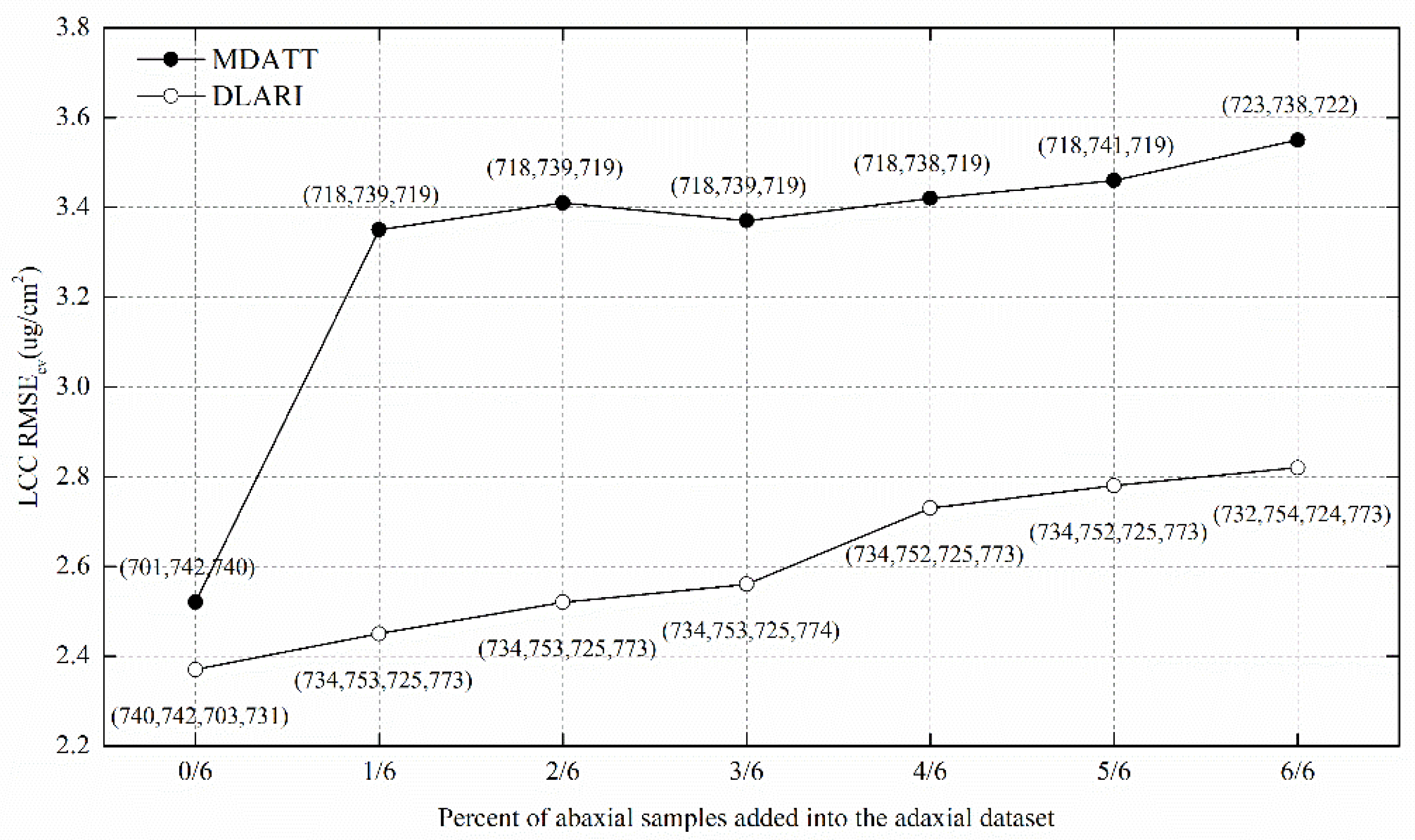
3.5. Comparison of the DLARI and MDATT

The difference between the MDATT and DLARI was the substitution of λ1 with an additional wavelength (λ4). We evaluated the improvement of incorporating this additional wavelength by calculating the maximum R2 of all band combinations for the DLARI formula based on the three datasets.
The maximum R2 was derived from combinations by fixing λ4 while changing λ1, λ2, and λ3 from 700 nm to 760 nm. The wavelength regions for λ4 were from 700 nm to 900 nm. The results are plotted in Figure 9. It shows that when λ4 was at 700 nm to 760 nm, the maximum R2 derived from adaxial DLARIs and abaxial DLARIs were similar to those of the adaxial MDATT (0.95) and abaxial MDATT (0.94), while bifacial DLARIs achieved higher correlations with LCC than the bifacial MDATT (0.91) since λ4 was higher than 709 nm. When λ4 was higher than 760 nm, all three DLARIs were much more correlated to LCC than the three MDATTs. The highest R2 of the adaxial DLARI and bifacial DLARI were obtained at λ4 equal to 819 nm and 773 nm, respectively, and then rapidly became lower than those of the MDATT when λ4 was located above 890 nm. For the abaxial dataset, the highest R2 appeared at λ4 equal to 774 nm and then became lower than the abaxial MDATT when λ4 was above 840 nm. Compared to the MDATT, the effective regions of λ4 for the adaxial DLARI were from 760 nm to 890 nm and for the abaxial DLARI when they were from 760 nm to 840 nm. For the bifacial DLARI, the robust wavelength regions of λ4 were from 709 nm to 890 nm.
The above bifacial DLARI was derived from a dataset composed of the same quantity of adaxial and abaxial reflectance measurements. In order to evaluate the impact of the abaxial reflectance on the performance of the two dorsiventral leaf adjusted indices, we divided the 84 abaxial reflectance samples into 6 parts and accumulated them into the adaxial dataset, then we calculated the optimal DLARIs and MDATTs and their accuracies, estimating LCC for each sub-dataset. The results are shown in Figure 10, which shows that the RMSEcv of MDATT dramatically increased from 2.52 to 3.35 when adding one-sixth of the abaxial samples into the adaxial dataset and then linearly increased to 3.55. With the increase of abaxial reflectance, the RMSEcv of DLARI stably increased from 2.37 to 2.82. Compared to the MDATT, the DLARI possessed a linear response to the impact of abaxial reflectance. The optimal wavelengths for the DLARI and MDATT derived from each sub-dataset showed unobvious changes with the addition of the abaxial reflectance. It can be concluded that the presence of abaxial leaves decreased the accuracy of DLARI and MDATT for LCC retrieval, but had no obvious influence on the optimal wavelengths for DLARI and MDATT.

4. Discussion

In the case of narrow band indices such as the MDATT, different wavelength combinations can provide the best performance for different vegetation types. Lu et al. [21] suggested the robust wavelength region for λ1 is from 723 to 885 nm and for λ2 and λ3 from 697 to 771 nm for woody plants. We optimized the wavelengths used in the MDATT to increase its suitability for peanut LCC estimation, but the effects from the dorsiventral leaf structure remained. The optimal wavelengths for the bifacial MDATT were 723 nm, 738 nm, and 722 nm. Using the MDATT as a basis, we constructed a DLARI to further decrease the impact of abaxial leaves. Compared with the MDATT and the published indices without considering the dorsiventral leaf structure, the three DLARIs performed best. The adaxial DLARI improved the estimation accuracy to 2.37 with a high R2 of 0.96. The abaxial DLARI achieved a performance with R2 = 0.95 and RMSE = 2.58. The bifacial DLARI showed an R2 value of 0.94 and RMSE of 2.81. The results showed that the DLARIs not only improved the retrieval of LCC from the adaxial side of the leaf, but also further reduced the impact of differences in the adaxial and abaxial leaf reflectance thus increasing LCC estimation from the bifacial reflectance.
The measured leaf reflectance can be composed of the external (surface) reflectance (Rs) of the leaf and internal reflectance (Ri) of the leaf [42]. The reflectance of the adaxial and abaxial leaf side differ both in the Rs and Ri. The MDATT and DLARI formulae both successfully removed Rs according to Equations (2) and (3), respectively. The left Ri is influenced by pigments concentrations and absorption properties which are different at the two sides of the leaf [16]. For the MDATT, the optimal wavelengths for λ1 and λ3 changed from 701 nm and 740 nm to 723 nm and 722 nm (Figure 10). The reflectance of the adaxial surface and abaxial surface at 723 nm and 722 nm showed minimum difference (Figure 2). The optimal wavelengths λ2 for bifacial MDATT was located at 738 nm where the reflectance of both sides showed similar sensitivity to LCC (Figure 3). The ability of MDATT to decrease the Ri effect contributed to the combination of these three wavelengths. For the DLARI, with the addition of abaxial samples into the adaxial dataset, the four wavelengths gradually changed to approximately 732 nm, 754 nm, 724 nm, and 773 nm (Figure 10). At 732 nm and 724 nm, the adaxial reflectance showed higher sensitivity to LCC than the abaxial reflectance. In contrast, at 754 nm and 773 nm, the abaxial reflectance showed stronger correlation to LCC than the adaxial reflectance (Figure 3). In addition, the optimal λ3 was located at the region where spectral differences among the two sides of the leaf were negligible (Figure 2). The wavelength near 754 nm is known as the red-edge shoulder and has shown considerable potential in suppressing the influence of leaf structure [43]. These factors contributed to DLARI being optimal for LCC estimation when bifacial reflectance measurements were used.
Compared to the published vegetation indices, the DLARI not only decreased the effect of dorsiventral leaf structure but also significantly improved LCC estimation from the adaxial reflectance measurements. In fact, when multiple bands are available, there is no reason to limit to two-band or three-band indices. For instance, the first three wavelengths used in the DLARI were similar to that used in the MDATT for the adaxial dataset, but the accuracy (RMSEcv) was improved from 2.52 to 2.37 by adding the fourth wavelength. Our results proved that indices based on four bands led to further improvements compared to two-band and three-band indices.
As previously mentioned, the reliability of narrow-band indices can be influenced by a range of phenotypic characteristics. Further work is required to assess the application of DLARI to estimate LCC for other crop species. The robust wavelength regions proposed should provide a good starting point for optimizing the index for other crop species.
The potential of satellites, such as Sentinel-2, to map crop biophysical variables has been shown by many studies [44,45]. The Sentinel-2 multispectral instrument includes three bands in the red-edge region centered at 705, 740, and 775 nm, which were found to be of great interest for crop monitoring [46]. Unmanned aerial vehicle (UAV) platforms coupled with imaging sensors are able to collect multispectral or hyperspectral imagery and offer great possibilities in the precision farming [47,48]. When using these remote sensing techniques to investigate peanut canopy information, the spectral information collected by the sensors may not only come from the adaxial leaf surfaces but also the abaxial leaf surfaces. Our results provide evidence that ignoring the spectral difference among the two faces introduces significant errors in LCC estimation. Further work should consider this effect when estimating peanut chlorophyll content or other biochemistry parameters at the canopy scale. The application of DLARI on remote sensing sensors to estimate canopy chlorophyll content is yet to be tested.

5. Conclusions

In this study, we focused on the development and optimization of dorsiventral leaf structure adjusted indices to minimize the impact of spectral differences between adaxial and abaxial leaf surfaces when retrieving peanut LCC. The wavelengths used by the MDATT were optimized for peanut, while a new dorsiventral leaf adjusted index was proposed to improve the LCC retrieval accuracy. The optimal MDATT index for retrieving LCC from bifacial reflectance measurements was ( R 723 R 738 ) / ( R 723 R 722 ) with an R2cv of 0.91 (RMSEcv = 3.53). The DLARI incorporated an additional wavelength in the NIR and exhibited the best retrieval accuracy when compared to the MDATT and other previously published indices. The DLARIs of ( R 735 R 753 ) / ( R 715 R 819 ) and ( R 732 R 754 ) / ( R 724 R 773 ) are recommended for retrieval of LCC using adaxial and bifacial reflectance, respectively. These two DLARIs delivered excellent cross-validation accuracies (R2cv = 0.96, RMSEcv = 2.37; R2cv = 0.94, RMSEcv = 2.81). The effective wavelength regions for DLARI were from the red edge to the NIR. Compared to the MDATT, the DLARI showed stronger correlation to LCC and less sensitivity to abaxial surface structure. This research provided new insights into the impact of spectral differences between adaxial and abaxial leaf surfaces on LCC estimation and proposed DLARI to improve LCC retrieval accuracy. The spectral differences between adaxial and abaxial leaf surfaces should be considered when estimating peanut canopy parameters. Further studies should be carried out to verify the applicability of DLARI to other plant species which have similar physiological response to solar radiation and drought stress as peanut.

Supplementary Materials

The following are available online at https://www.mdpi.com/2072-4292/11/18/2148/s1, Figure S1: Photographs of peanut canopies in the field.

Author Contributions

Conceptualization, Y.D., M.X. and Z.W.; methodology, Y.D. and M.X.; formal analysis, M.X. and Y.D.; data curation, H.W.; writing—original draft preparation, M.X. and Y.D.; writing—review and editing, A.H., L.A.B., Q.X. and X.X.; funding acquisition, Z.W.

Funding

This research was funded by the National Key Research and Development Program of China, grant number 2016YFD0200102, the Technology Development Program of Jilin Province, China, grant number 20180201012GX and “The 13th Five-Year plan” Science and Technology Project of the Department of Education, Jilin Province, grant number JJKH20170915KJ.

Acknowledgments

The support provided by the China Scholarship Council (CSC) during a visit by Yanling Ding (No.201806625001) to the University of Technology Sydney is acknowledged. The authors would like to thank the editors and reviewers who handled our paper.

Conflicts of Interest

The authors declare no conflict of interest.

References

  1. FAOSTAT. 2017. Available online: http://www.fao.org (accessed on 21 May 2019).
  2. Akram, N.A.; Shafiq, F.; Ashraf, M. Peanut (Arachis hypogaea L.): A prospective legume crop to offer multiple health benefits under changing climate. Compr. Rev. Food Sci. Food Saf. 2018, 17, 1325–1338. [Google Scholar] [CrossRef]
  3. Wu, C.; Niu, Z.; Tang, Q.; Huang, W. Estimating chlorophyll content from hyperspectral vegetation indices: Modeling and validation. Agric. For. Meteorol. 2008, 148, 1230–1241. [Google Scholar] [CrossRef]
  4. Daughtry, C.S.T.; Walthall, C.L.; Kim, M.S.; de Colstoun, E.B.; McMurtrey, J.E. Estimating corn leaf chlorophyll concentration from leaf and canopy reflectance. Remote Sens. Environ. 2000, 74, 229–239. [Google Scholar] [CrossRef]
  5. Anjum, S.A.; Xie, X.Y.; Wang, L.C.; Saleem, M.F.; Man, C.; Lei, W. Morphological, physiological and biochemical responses of plants to drought stress. Afr. J. Agric. Res. 2011, 6, 2026–2032. [Google Scholar]
  6. Mulla, D.J. Twenty five years of remote sensing in precision agriculture: Key advances and remaining knowledge gaps. Biosyst. Eng. 2013, 114, 358–371. [Google Scholar] [CrossRef]
  7. Hunt, E.R.; Doraiswamy, P.C.; McMurtrey, J.E.; Daughtry, C.S.T.; Perry, E.M.; Akhmedov, B. A visible band index for remote sensing leaf chlorophyll content at the canopy scale. Int. J. Appl. Earth Obs. Geoinf. 2013, 21, 103–112. [Google Scholar] [CrossRef] [Green Version]
  8. Verrelst, J.; Malenovský, Z.; Van der Tol, C.; Camps-Valls, G.; Gastellu-Etchegorry, J.-P.; Lewis, P.; North, P.; Moreno, J. Quantifying vegetation biophysical variables from imaging spectroscopy data: A review on retrieval methods. Surv. Geophys. 2019, 40, 589–629. [Google Scholar] [CrossRef]
  9. Féret, J.-B.; François, C.; Gitelson, A.; Asner, G.P.; Barry, K.M.; Panigada, C.; Richardson, A.D.; Jacquemoud, S. Optimizing spectral indices and chemometric analysis of leaf chemical properties using radiative transfer modeling. Remote Sens. Environ. 2011, 115, 2742–2750. [Google Scholar] [CrossRef] [Green Version]
  10. Malenovský, Z.; Homolová, L.; Zurita-Milla, R.; Lukeš, P.; Kaplan, V.; Hanuš, J.; Gastellu-Etchegorry, J.-P.; Schaepman, M.E. Retrieval of spruce leaf chlorophyll content from airborne image data using continuum removal and radiative transfer. Remote Sens. Environ. 2013, 131, 85–102. [Google Scholar] [CrossRef] [Green Version]
  11. Ustin, S.L.; Gitelson, A.A.; Jacquemoud, S.; Schaepman, M.; Asner, G.P.; Gamon, J.A.; Zarco-Tejada, P. Retrieval of foliar information about plant pigment systems from high resolution spectroscopy. Remote Sens. Environ. 2009, 113, S67–S77. [Google Scholar] [CrossRef] [Green Version]
  12. Datt, B. A new reflectance index for remote sensing of chlorophyll content in higher plants: Tests using eucalyptus leaves. J. Plant Physiol. 1999, 154, 30–36. [Google Scholar] [CrossRef]
  13. Sims, D.A.; Gamon, J.A. Relationships between leaf pigment content and spectral reflectance across a wide range of species, leaf structures and developmental stages. Remote Sens. Environ. 2002, 81, 337–354. [Google Scholar] [CrossRef]
  14. Gitelson, A.A.; Gritz †, Y.; Merzlyak, M.N. Relationships between leaf chlorophyll content and spectral reflectance and algorithms for non-destructive chlorophyll assessment in higher plant leaves. J. Plant Physiol. 2003, 160, 271–282. [Google Scholar] [CrossRef] [PubMed]
  15. Kalariya, K.A.; Singh, A.L.; Goswami, N.; Mehta, D.; Mahatma, M.K.; Ajay, B.C.; Chakraborty, K.; Zala, P.V.; Chaudhary, V.; Patel, C.B. Photosynthetic characteristics of peanut genotypes under excess and deficit irrigation during summer. Physiol. Mol. Biol. Plants 2015, 21, 317–327. [Google Scholar] [CrossRef] [PubMed] [Green Version]
  16. Hlavinka, J.; Nauš, J.; Špundová, M. Anthocyanin contribution to chlorophyll meter readings and its correction. Photosynth. Res. 2013, 118, 277–295. [Google Scholar] [CrossRef] [PubMed]
  17. Stuckens, J.; Verstraeten, W.W.; Delalieux, S.; Swennen, R.; Coppin, P. A dorsiventral leaf radiative transfer model: Development, validation and improved model inversion techniques. Remote Sens. Environ. 2009, 113, 2560–2573. [Google Scholar] [CrossRef]
  18. Baránková, B.; Lazár, D.; Nauš, J. Analysis of the effect of chloroplast arrangement on optical properties of green tobacco leaves. Remote Sens. Environ. 2016, 174, 181–196. [Google Scholar] [CrossRef]
  19. Lu, X.; Lu, S. Effects of adaxial and abaxial surface on the estimation of leaf chlorophyll content using hyperspectral vegetation indices. Int. J. Remote Sens. 2015, 36, 1447–1469. [Google Scholar] [CrossRef]
  20. Lu, S.; Lu, X.; Zhao, W.; Liu, Y.; Wang, Z.; Omasa, K. Comparing vegetation indices for remote chlorophyll measurement of white poplar and Chinese elm leaves with different adaxial and abaxial surfaces. J. Exp. Bot. 2015, 66, 5625–5637. [Google Scholar] [CrossRef] [Green Version]
  21. Lu, S.; Lu, F.; You, W.; Wang, Z.; Liu, Y.; Omasa, K. A robust vegetation index for remotely assessing chlorophyll content of dorsiventral leaves across several species in different seasons. Plant Methods 2018, 14, 15. [Google Scholar] [CrossRef]
  22. Dash, J.; Curran, P.J. The MERIS terrestrial chlorophyll index. Int. J. Remote Sens. 2004, 25, 5403–5413. [Google Scholar] [CrossRef]
  23. Huete, A.; Didan, K.; Miura, T.; Rodriguez, E.P.; Gao, X.; Ferreira, L.G. Overview of the radiometric and biophysical performance of the MODIS vegetation indices. Remote Sens. Environ. 2002, 83, 195–213. [Google Scholar] [CrossRef]
  24. Verrelst, J.; Rivera, J.P.; Veroustraete, F.; Muñoz-Marí, J.; Clevers, J.G.P.W.; Camps-Valls, G.; Moreno, J. Experimental Sentinel-2 LAI estimation using parametric, non-parametric and physical retrieval methods—A comparison. ISPRS J. Photogramm. Remote Sens. 2015, 108, 260–272. [Google Scholar] [CrossRef]
  25. Wang, W.; Yao, X.; Yao, X.; Tian, Y.; Liu, X.; Ni, J.; Cao, W.; Zhu, Y. Estimating leaf nitrogen concentration with three-band vegetation indices in rice and wheat. Field Crop. Res. 2012, 129, 90–98. [Google Scholar] [CrossRef]
  26. Xie, Q.; Dash, J.; Huang, W.; Peng, D.; Qin, Q.; Mortimer, H.; Casa, R.; Pignatti, S.; Laneve, G.; Pascucci, S.; et al. Vegetation indices combining the red and red-edge spectral information for leaf area index retrieval. IEEE J. Sel. Top. Appl. Earth Obs. Remote Sens. 2018, 11, 1482–1493. [Google Scholar] [CrossRef]
  27. Brown, L.A.; Dash, J.; Lidón, A.L.; Lopez-Baeza, E.; Dransfeld, S. Synergetic exploitation of the Sentinel-2 missions for validating the Sentinel-3 ocean and land color instrument terrestrial chlorophyll index over a vineyard dominated mediterranean environment. IEEE J. Sel. Top. Appl. Earth Obs. Remote Sens. 2019, 12, 2244–2251. [Google Scholar] [CrossRef]
  28. Dash, J.; Curran, P.J.; Tallis, M.J.; Llewellyn, G.M.; Taylor, G.; Snoeij, P. Validating the MERIS Terrestrial Chlorophyll Index (MTCI) with ground chlorophyll content data at MERIS spatial resolution. Int. J. Remote Sens. 2010, 31, 5513–5532. [Google Scholar] [CrossRef] [Green Version]
  29. Vuolo, F.; Dash, J.; Curran, P.J.; Lajas, D.; Kwiatkowska, E. Methodologies and uncertainties in the use of the terrestrial chlorophyll index for the Sentinel-3 mission. Remote Sens. 2012, 4, 1112–1133. [Google Scholar] [CrossRef]
  30. Kong, W.; Huang, W.; Liu, J.; Chen, P.; Qin, Q.; Ye, H.; Peng, D.; Dong, Y.; Mortimer, A.H. Estimation of canopy carotenoid content of winter wheat using multi-angle hyperspectral data. Adv. Space Res. 2017, 60, 1988–2000. [Google Scholar] [CrossRef]
  31. Sartory, D.P.; Grobbelaar, J.U. Extraction of chlorophyll a from freshwater phytoplankton for spectrophotometric analysis. Hydrobiologia 1984, 114, 177–187. [Google Scholar] [CrossRef]
  32. Arnon, D.I. Copper enzymes in isolated chloroplasts. polyphenol oxidase in beta vulgaris. Plant Physiol. 1949, 24, 1–15. [Google Scholar] [CrossRef] [PubMed]
  33. Baret, F.; Andrieu, B.; Guyot, G. A simple model for leaf optical properties in visible and near-infrared: Application to the analysis of spectral shifts determinism. In Applications of Chlorophyll Fluorescence in Photosynthesis Research, Stress Physiology, Hydrobiology and Remote Sensing; Springer: Dordrecht, The Netherlands, 1988; pp. 345–351. [Google Scholar]
  34. Main, R.; Cho, M.A.; Mathieu, R.; O’Kennedy, M.M.; Ramoelo, A.; Koch, S. An investigation into robust spectral indices for leaf chlorophyll estimation. ISPRS J. Photogramm. Remote Sens. 2011, 66, 751–761. [Google Scholar] [CrossRef]
  35. Drusch, M.; Del Bello, U.; Carlier, S.; Colin, O.; Fernandez, V.; Gascon, F.; Hoersch, B.; Isola, C.; Laberinti, P.; Martimort, P.; et al. Sentinel-2: ESA’s Optical High-Resolution Mission for GMES Operational Services. Remote Sens. Environ. 2012, 120, 25–36. [Google Scholar] [CrossRef]
  36. Vogelmann, J.E.; Rock, B.N.; Moss, D.M. Red edge spectral measurements from sugar maple leaves. Int. J. Remote Sens. 1993, 14, 1563–1575. [Google Scholar] [CrossRef]
  37. Carter, G.A. Ratios of leaf reflectances in narrow wavebands as indicators of plant stress. Int. J. Remote Sens. 1994, 15, 697–703. [Google Scholar] [CrossRef]
  38. Maccioni, A.; Agati, G.; Mazzinghi, P. New vegetation indices for remote measurement of chlorophylls based on leaf directional reflectance spectra. J. Photochem. Photobiol. B Biol. 2001, 61, 52–61. [Google Scholar] [CrossRef]
  39. Guyot, G.; Baret, F. Utilisation de la haute resolution spectrale pour suivre l’etat des couverts vegetaux. In Proceedings of the Spectral Signatures of Objects in Remote Sensing, Modane, France, 18–22 January 1988; p. 279. [Google Scholar]
  40. Meyer, H.; Lehnert, L.W.; Wang, Y.; Reudenbach, C.; Nauss, T.; Bendix, J. From local spectral measurements to maps of vegetation cover and biomass on the Qinghai-Tibet-Plateau: Do we need hyperspectral information? Int. J. Appl. Earth Obs. Geoinf. 2017, 55, 21–31. [Google Scholar] [CrossRef]
  41. Reicosky, D.A.; Hanover, J.W. Physiological effects of surface waxes. Plant Physiol. 1978, 62, 101–104. [Google Scholar] [CrossRef]
  42. McClendon, J.H.; Fukshansky, L. On the interpretation of absorption spectra of leaves–I. Introduction and the correction of leaf spectra for surface reflection. Photochem. Photobiol. 1990, 51, 203–210. [Google Scholar] [CrossRef]
  43. Croft, H.; Chen, J.M.; Zhang, Y. The applicability of empirical vegetation indices for determining leaf chlorophyll content over different leaf and canopy structures. Ecol. Complex. 2014, 17, 119–130. [Google Scholar] [CrossRef]
  44. Kross, A.; McNairn, H.; Lapen, D.; Sunohara, M.; Champagne, C. Assessment of RapidEye vegetation indices for estimation of leaf area index and biomass in corn and soybean crops. Int. J. Appl. Earth Obs. Geoinf. 2015, 34, 235–248. [Google Scholar] [CrossRef] [Green Version]
  45. Xie, Q.; Dash, J.; Huete, A.; Jiang, A.; Yin, G.; Ding, Y.; Peng, D.; Hall, C.C.; Brown, L.; Shi, Y.; et al. Retrieval of crop biophysical parameters from Sentinel-2 remote sensing imagery. Int. J. Appl. Earth Obs. Geoinf. 2019, 80, 187–195. [Google Scholar] [CrossRef]
  46. Delloye, C.; Weiss, M.; Defourny, P. Retrieval of the canopy chlorophyll content from Sentinel-2 spectral bands to estimate nitrogen uptake in intensive winter wheat cropping systems. Remote Sens. Environ. 2018, 216, 245–261. [Google Scholar] [CrossRef]
  47. Kanning, M.; Kühling, I.; Trautz, D.; Jarmer, T. High-Resolution UAV-Based Hyperspectral Imagery for LAI and Chlorophyll Estimations from Wheat for Yield Prediction. Remote Sens. 2018, 10, 2000. [Google Scholar] [CrossRef]
  48. Tahir, N.; Naqvi, S.M.; Lan, Y.; Zhang, Y.; Wang, Y.; Afzal, M.; Cheema, M.J. Real time monitoring chlorophyll content based on vegetation indices derived from multispectral UAVs in the kinnow orchard. Int. J. Precis. Agric. Aviat. 2018, 1, 24–31. [Google Scholar] [CrossRef]
Figure 1. Photographs of the peanut canopy in the field. Only the adaxial surface is visible under low solar irradiance (a), while both the adaxial and abaxial surfaces are visible under high solar irradiance (b).
Remotesensing 11 02148 g001
Figure 2. The spectral reflectance of the adaxial and abaxial surfaces (a) and the associated difference in reflectance among the two sides (b). (The solid line represents the mean of sampled reflectance and the shaded zone represents standard deviation).
Remotesensing 11 02148 g002
Figure 3. Optical micrographs of the adaxial (a) and abaxial (b) surface of peanut leaves.
Remotesensing 11 02148 g003
Figure 4. The correlation between LCC and the reflectance of the adaxial and abaxial surfaces from 350 to 2500 nm.
Remotesensing 11 02148 g004
Figure 5. The maximum R2 values associated with the MDATT band combinations ranging from 400 nm to 1000 nm (ac) and its corresponding λ1 (df). The left column is for the adaxial dataset, the middle column is for the abaxial dataset, and the right column is for the bifacial dataset. For the sake of concise display, only R2 values greater than 0.8 were considered.
Remotesensing 11 02148 g005
Figure 6. Relationships between MDATTs and LCC (ac) and scatter plots between observed LCC and LCC predicted by the associated linear models (df). The different colors indicate the 10 fold cross-validation subsets. The left column is for the adaxial dataset, the middle column is for the abaxial dataset, and the right column is for the bifacial dataset.
Remotesensing 11 02148 g006
Figure 7. Relationships between optimal DLARI indices and LCC (ac) and scatter plots between observed LCC and LCC predicted by the associated linear models (df). The different colors indicate the 10 fold cross-validation subsets. The left column is for the adaxial dataset, the middle column is for the abaxial dataset, and the right column is for the bifacial dataset.
Remotesensing 11 02148 g007
Figure 8. Comparison of published vegetation indices and the indices developed in this study for LCC estimation using adaxial and bifacial reflectance measurements.
Remotesensing 11 02148 g008
Figure 9. Maximum R2 between LCC and MDATTs, DLARIs with λ1, λ2, and λ3 from 700 nm to 760 nm and λ4 from 700 nm to 900 nm.
Remotesensing 11 02148 g009
Figure 10. The impact of the dorsiventral leaf structure on DLARI and MDATT in terms of the estimation accuracy and optimal wavelengths. The numbers in the brackets are the optimal wavelengths for DLARI and MDATT with a unit of nm.
Remotesensing 11 02148 g010
Table 1. The list of the published vegetation indices compared in the study.
IndexAbbreviationFormulaScaleReference
Gitelson’s index Gitelson1/R700Leaf[35]
Vogelmann’s first IndexVOG1R740/R720Leaf[36]
Carter’ IndexCarterR710/R760Leaf [37]
MERIS Terrestrial Chlorophyll IndexMTCI(R740 − R705)/(R705 − R665)Canopy[22]
Modified Simple Ratio mSR705(R750 − R445)/(R705 − R445)Leaf[13]
Modified Normalized Difference Vegetation IndexmND705(R750 − R705)/(R750 + R705 − 2 × R445)Leaf[13]
Datt’ IndexDATT(R850 − R710)/(R850 − R680)Leaf[12]
Maccioni’ IndexMaccioni(R780 − R710)/(R780 − R680)Leaf[38]
Vogelmann’s second IndexVOG2(R734 − R747)/(R715 + R720)Leaf[36]
Red-Edge Position IndexREP700 + 40 × (((R670 + R780)/2 − R700)/(R740 − R700))Leaf[39]
Modified Datt IndexLu′s MDATT(R691 − R7745)/(R7691 − R745)Leaf[21]
Modified Datt IndexLu′s MDATT(R721 − R744)/(R721 − R714)Leaf[21]
Table 2. Cross-validation results for the MDATT indices in the case of the adaxial, abaxial, and bifacial datasets.
IndexDatasetWavelength Region Considered
(nm)
Optimal Wavelengths
(nm)
R2R2cvRMSEcv
(μg/cm2)
MDATTAdaxial reflectance400–1000λ1: 701; λ2: 742; λ3: 7400.950.952.52
Abaxial reflectance400–1000λ1: 718; λ2: 747; λ3: 7200.940.942.69
Bifacial reflectance400–1000λ1: 723; λ2: 738; λ3: 7220.910.913.53
Table 3. LCC retrieval accuracy of the adaxial and bifacial MDATT indices when applied to bifacial dataset.
Dataset Adaxial MDATTBifacial MDATT
R2cvRMSEcv (μg/cm2)R2cvRMSEcv (μg/cm2)
Bifacial reflectance0.874.140.913.53
Table 4. Cross-validation results for the optimal dorsiventral leaf adjusted ratio indices (DLARIs) derived using wavelengths between 660 and 750 nm in the case of the adaxial, abaxial, and bifacial datasets.
IndexDatasetWavelength Region Considered
(nm)
Optimal Wavelengths
(nm)
R2R2cvRMSEcv
(μg/cm2)
DLARIAdaxial reflectance660–750λ1: 740; λ2: 742; λ3: 703; λ4: 7310.950.952.53
Abaxial reflectance660–750λ1: 714; λ2: 746; λ3: 718; λ4: 7200.940.942.62
Bifacial reflectance660–750λ1: 731; λ2: 741; λ3: 722; λ4: 7500.910.923.34
Table 5. Cross-validation results for the optimal DLARIs derived using wavelengths between 660 and 820 nm in the case of the adaxial, abaxial, and bifacial datasets.
IndexDatasetWavelength Region Considered
(nm)
Optimal Wavelengths
(nm)
R2R2cvRMSEcv
(μg/cm2)
DLARIAdaxial reflectance660–820λ1: 735; λ2: 753; λ3: 715; λ4: 8190.960.962.37
Abaxial reflectance660–820λ1: 731; λ2: 755; λ3: 722; λ4: 7740.950.952.58
Bifacial reflectance660–820λ1: 732; λ2: 754; λ3: 724; λ4: 7730.940.942.81

