Mitigation of Unmodeled Error to Improve the Accuracy of Multi-GNSS PPP for Crustal Deformation Monitoring

Abstract

High-rate multi-constellation global navigation satellite system (GNSS) precise point positioning (PPP) has been recognized as an efficient and reliable technique for large earthquake monitoring. However, the displacements derived from PPP are often overwhelmed by the centimeter-level noise, therefore they are usually unable to detect slight deformations which could provide new findings for geophysics. In this paper, Global Positioning System (GPS), GLObalnaya NAvigatsionnaya Sputnikovaya Sistema (GLONASS), and BeiDou navigation satellite system (BDS) data collected during the 2017 Mw 6.5 Jiuzhaigou earthquake were used to further exploit the capability of BDS-only and multi-GNSS PPP in deformation monitoring by applying sidereal filtering (SF) in the observation domain. The equation that unifies the residuals for the uncombined and undifferenced (UCUD) PPP solution on different frequencies was derived, which could greatly reduce the complexity of data processing. An unanticipated long-term periodic error term of up to ± 3 cm was found in the phase residuals associated with BDS satellites in geostationary Earth orbit (GEO), which is not due to multipath originated from the ground but is in fact satellite dependent. The period of this error is mainly longer than 2000 s and cannot be alleviated by using multi-GNSS. Compared with solutions without sidereal filtering, the application of the SF approach dramatically improves the positioning precision with respect to the weekly averaged positioning solution, by 75.2%, 42.8%, and 56.7% to 2.00, 2.23, and 5.58 cm in the case of BDS-only PPP in the east, north, and up components, respectively, and 71.2%, 27.7%, and 37.9% to 1.25, 0.81, and 3.79 cm in the case of GPS/GLONASS/BDS combined PPP, respectively. The GPS/GLONASS/BDS combined solutions augmented by the SF successfully suppress the GNSS noise, which contributes to the detection of the true seismic signal and is beneficial to the pre- and post-seismic signal analysis.

1. Introduction

High-rate global navigation satellite systems (GNSSs) have shown great potential in observing both ground static and dynamic motions, which is more than a favorable complement to traditional seismometers [1,2]. Retrieving high-precision coseismic displacement in real time contributes significantly to rapid source and rupture inversion [3,4], rapid hazard assessment [5], and early warning of earthquake [6].

Typically, there are two primary techniques for real-time GNSS data processing. One is the relative positioning technique, which is able to achieve a positioning accuracy better than 1 cm when satellite orbits and clocks, as well as atmosphere errors, are basically eliminated through observation differences between two nearby stations [7]. The limitation is, however, that only relative displacement can be obtained with respect to the reference station, which might itself be subject to shaking in the case of a large earthquake. On the contrary, precise point positioning (PPP) can provide absolute precise position with respect to a global reference frame using a single Global Positioning System (GPS) receiver [8], and has been therefore widely used for seismo-geodesy in recent years [9,10]. Compared with the traditional ionosphere-free combination PPP, the uncombined and undifferenced (UCUD) PPP using raw observations can retain all meaningful information and be easily extended to multi-frequency processing. Thus, it is a popularly adopted PPP model [11,12]. In some cases, the high-rate PPP has the capability of generating kinematic position estimates at millimeter level if it is only quantifying a short period of data under favorable observation circumstances [13,14]. In general, the 3-D displacement estimate is believed to have an accuracy of a few to ten centimeters, which hinders deep insights into rupture processes as well as possible geophysics findings.

Previous studies have indicated that one of the major errors causing positioning precision deterioration is the multipath, which can transform into other parameters such as positions, tropospheric parameters, and float ambiguity terms, and primarily dominates on the low-frequency band over a few tens of seconds to minutes [15,16]. Multipath effects cannot simply average out over a limited period of data, and probably induce spurious seismic signals as well as bias the coseismic displacement estimations. According to the spatiotemporal repeatability of multipath under static environments, two prevalent approaches were proposed to mitigate the multipath impacts on high-rate GNSS in the observation domain. For the multipath hemispherical map (MHM), the multipath is assumed to be dependent on the specific elevation and azimuth angle of the satellite [17], and it can be used for real-time application [18]. The sidereal filtering (SF) approach calculates the multipath corrections from neighboring days, and then subtracts the time-shift corrections from the observations on the day of interest based on satellite orbital repeat time [19]. This method is capable of capturing higher-frequency multipath and is more suitable for seismic waveform detection. As the multipath is frequency dependent and has a time lag for different frequencies, it is necessary to build a correction model for each frequency [20]. Therefore, it complicates the implementation of data processing for multi-frequency, especially for GLObalnaya NAvigatsionnaya Sputnikovaya Sistema (GLONASS), which has inter-frequency bias (IFB) among satellites. In addition to the multipath, the errors of satellite orbits and clocks and the atmospheric delays still remain in the phase residuals [21,22], which could affect the performance of the SF approach to some extent.

In spite of numerous studies about the performance of multi-GNSS PPP, only a few have investigated the multipath effects on PPP [16,22]. In addition, the new BeiDou navigation satellite system (BDS) performs comparably to GPS in the relative positioning aspect but is inferior for PPP [23,24,25,26]. Based on the above analysis, this paper aimed to exploit high-rate multi-GNSS observations to improve the precision of displacement estimates, especially in the case of BDS. The equations describing the relationship between phase residuals on different frequencies were rigorously derived and validated. The characteristics of BDS residuals were investigated in detail to identify potential problems that could hinder the precision and reliability of the BDS-only PPP. Afterward, the multipath corrections were calculated using the SF approach based on the phase residuals for each satellite. Then, the performance of multi-GNSS UCUD PPP augmented by the SF approach, especially of the BDS-only PPP, was assessed using Jiuzhaigou earthquake data.

The rest of the paper is organized as follows. The description of the multi-GNSS PPP data processing strategy is given first in Section 2. Afterward, the equations that describe the relationship between phase residuals on different frequencies are derived. Section 3 presents the multi-GNSS data description. Section 4 displays the analysis of the characteristics of BDS geostationary Earth orbit (GEO) phase residuals, PPP solutions using sidereally filtered multi-GNSS data, especially BDS PPP solutions, and a case study on the Jiuzhaigou earthquake. Finally, in Section 5, the conclusions and perspectives are provided.

2. Methodology

2.1. PPP Model and Data Processing Strategy

After correcting the satellite orbits and clocks using the precise products, the PPP model for GPS, GLONASS, and BDS can be written as follows:

$$\{\begin{array}{l}{p}_{r,\mathrm{j}}^G=-e_r^G\cdot r_r^{}+{\overline{\mathrm{t}}}_r^{}+{\gamma }_{j,G}^{}{\overline{I}}_{r,1}^G+T_r^G+M_{r,\mathrm{j}}^G+{\xi }_{r,j}^G\\ p_{r,\mathrm{j}}^{Rk}=-e_r^{Rk}\cdot r_r^{}+{\overline{\mathrm{t}}}_r^{}+{\delta }_{r,\mathrm{Rk}}^{}+{\gamma }_{j,Rk}^R{\overline{I}}_{r,1}^{Rk}+T_r^R+M_{r,\mathrm{j}}^{Rk}+{\xi }_{r,j}^{Rk}\\ p_{r,\mathrm{j}}^C=-e_r^C\cdot r_r^{}+{\overline{\mathrm{t}}}_r^{}+{\delta }_{r,\mathrm{C}}^{}+{\gamma }_{j,\mathrm{C}}^{}{\overline{I}}_{r,1}^C+T_r^C+M_{r,\mathrm{j}}^C+{\xi }_{r,j}^C\end{array},$$

(1)

$$\{\begin{array}{l}{l}_{r,j}^G=-e_r^G\cdot r_r^{}+{\overline{\mathrm{t}}}_r^{}-{\gamma }_{j,G}^{}{\overline{I}}_{r,1}^G+T_r^G+{\lambda }_j^G{\overline{N}}_{r,j}^G+m_{r,j}^G+{\epsilon }_{r,j}^G\\ l_{r,j}^{R_k}=-e_r^{R_k}\cdot r_r^{}+{\overline{\mathrm{t}}}_r^{}+{\delta }_{r,{\mathrm{R}}_{\mathrm{k}}}^{}-{\gamma }_{j,{\mathrm{R}}_k}^{}{\overline{I}}_{r,1}^R+T_r^R+{\lambda }_{j,R_k}^R{\overline{N}}_{r,j}^R+m_{r,j}^{R_k}+{\epsilon }_{r,j}^R\\ l_{r,j}^C=-e_r^C\cdot r_r^{}+{\overline{\mathrm{t}}}_r^{}+{\delta }_{r,\mathrm{C}}^{}-{\gamma }_{j,\mathrm{C}}^{}{\overline{I}}_{r,1}^C+T_r^C+{\lambda }_j^C{\overline{N}}_{r,j}^C+m_{r,j}^C+{\epsilon }_{r,j}^C\end{array},$$

(2)

where $p_{r,\mathrm{j}}^s$ and $l_{r,j}^s$ are the “observed minus computed” pseudo-range and phase observations from receiver $r$ to satellite $s$ on frequency $j(j=1,2)$; the superscripts G, R, and C represent the GPS, GLONASS, and BDS systems, respectively; $R_k^{}$ denotes the frequency factor of the GLONASS satellite; $e_r^s$ is the line-of-sight unit vector from receiver to satellite; $r_r^{}$ denotes the vector of the receiver position increments with respect to the a priori position used for linearization; ${\overline{\mathrm{t}}}_r^{}$ is the receiver clock offset; ${\delta }_{r,\mathrm{C}}^{}$ and ${\delta }_{r,{\mathrm{R}}_{\mathrm{k}}}^{}$ denote the inter-system bias (ISB) with respect to GPS and the inter-frequency bias (IFB) for GLONASS, respectively; and ${\overline{N}}_{r,j}^{\mathrm{s}}$ refers to the float ambiguity containing code hardware and phase delay, while ${\lambda }_j^s$ is its corresponding wavelength. The ionospheric delay at different frequencies can be expressed as ${\overline{I}}_{r,j}^s={\gamma }_{j,s}^{}{\overline{I}}_{r,1}^s,{\gamma }_{j,s}^{}=f_1^2/f_j^2$; $T_r^s$ denotes the slant tropospheric delay; $M_{r,\mathrm{j}}^s$ and $m_{r,\mathrm{j}}^s$ represent the multipaths in pseudo-range and carrier-phase observations; and ${\xi }_{r,j}^s$ and ${\epsilon }_{r,j}^s$ are the measurement noises. Other error items, such as the phase wind-up, relativity effects, Earth rotation, and tidal loading, are corrected by applying models described in Kouba [27]. It should be noted that, for GPS and GLONASS, the phase center offsets and variations (PCO and PCV) at both satellite and receiver are obtained from the International GNSS Service (IGS) antenna file. On the other hand, for BDS, the PCO and PCV at satellite are available from the IGS antenna file, but replaced by GPS at the receiver [28]. The data processing information is listed in

Table 1. Data processing information for multi-global navigation satellite system (GNSS) precise point positioning (PPP).

Item	Processing Information
Estimator	Least-squares estimator for generating phase residuals
Observations	Raw pseudo-range and carrier-phase observations from GPS, GLONASS, and BDS
Sampling rate	1 s
Elevation cutoff	7°
Weighting scheme	Elevation-dependent weight; 3 dm and 3 mm for GPS pseudo-range and carrier-phase; 4.5 dm and 3 mm for GLONASS pseudo-range and carrier-phase; 9.0 dm for BDS pseudo-range; and 5 mm and 15 mm for IGSO/MEO and GEO carrier-phase, respectively
Satellite orbit/clock	GBM final precise orbit/clock products generated by GFZ (Deng et al. [29])
Tropospheric delay	The zenith hydrostatic delay corrected by Saastamoinen’s model [30]; the zenith wet delay and the horizontal gradients estimated as piecewise constants every hour and six hours, respectively; Global Mapping Function (GMF) applied
Ionospheric delay	Estimated epoch by epoch
Satellite/Receiver antenna phase center	GPS/GLONASS: Corrected both at satellite and receiver BDS: PCO and PCV corrected at satellite, while replaced by GPS at receiver
Phase-windup effect	Corrected
ISB and IFB	ISB estimated as white noise, GPS as reference, whereas IFB estimated as constant for a whole day
Station displacement	Solid Earth tide, pole tide, ocean tide loading, IERS Convention 2010
Receiver coordinate	Estimated as constants for daily solution
Receiver clock	Estimated as white noise
Ambiguity	Estimated as constant for each arc: float value

GPS, Global Positioning System; GLONASS, GLObalnaya NAvigatsionnaya Sputnikovaya Sistema; BDS, BeiDou navigation satellite system; IGSO, Inclined Geosynchronous Orbit; MEO, Medium Earth Orbit; GEO, Geostationary Earth Orbit; GFZ, German Research Centre for Geosciences; PCO, phase center offsets; PCV, phase center variations; ISB, inter-system bias; IFB, inter-frequency bias; IERS, International Earth Rotation and Reference Systems Service.

in detail. The receiver clock offset is treated as white noise, and estimated epoch by epoch. Together with other parameters, the receiver positions are estimated as daily solution using the least-squares estimator.

For the SF method, the satellite orbital repeat times for GPS and BDS satellites are computed individually using Keplerian orbital elements from broadcast ephemerides [19,31]. On the other hand, for GLONASS, its broadcast ephemeris is presented by positions and velocities, and thus we used the aspect repeat time instead [32,33]. The phase residuals over n days before the day of interest are shifted by n times the orbital repeat time and then stacked for each station–satellite pair. Afterward, these stacked residuals are low-pass filtered with a cutoff frequency of 10 s to generate multipath corrections since any prominent multipath over shorter periods are not anticipated [34]. Finally, the phase observations on the day of interest are corrected, and then processed by the forward Kalman filter for simulating the kinematic PPP in real time.

2.2. Mathematic Relationship of Residuals on Different Frequencies

Since the coordinates are fixed and the zenith tropospheric delays and ambiguities are treated as constants during a period of time, the residuals, which are primarily the multipath errors, are related to the time-varying parameters, that is, receiver clock and ionospheric delays. Therefore, Equation (2) can be rearranged as follows:

$$V=AX-L,$$

(3)

$$A=\left[\begin{array}{l}E-I\\ E-{\gamma }_2^{}\cdot I\end{array}\right],X=\left[\begin{array}{l}{\overline{t}}_r\\ {\overline{I}}_1^s\end{array}\right],L=\left[\begin{array}{l}{\overline{l}}_1^s\\ {\overline{l}}_2^s\end{array}\right],V=\left[\begin{array}{l}{v}_1^s\\ v_2^s\end{array}\right],$$

(4)

where $A$ denotes the design matrix; $E$ denotes a column vector of n-dimension with value one; $I$ is an identity matrix of n-dimension; $X$ is the parameter vector of receiver clock and ionospheric delays; $L$ refers to the vector of unmodeled errors, and each element of ${\overline{l}}_j^s$ can be expressed as $l_j^s+e_r^s\cdot r_r^{}-T_r^s-{\lambda }_j^s{\overline{N}}_j^s$; and $V$ represents the vector of residuals. According to the least-squares criterion, the estimated parameters read as follows:

$$\widehat{X}={(A^{T}A)}^{-1}{A}^{T}L.$$

(5)

By substituting Equation (5) into (3), the residuals are derived:

$$V=(A(A_{}^{T}A{)}^{-1}{A}^T-I)L.$$

(6)

The term $A_{}^{T}A$ can also be simplified as follows:

$$A_{}^{T}A=\left[\begin{array}{l}{a}_{11}^{}{a}_{12}^{}\\ a_{21}^{}{a}_{22}^{}\end{array}\right],$$

(7)

where $a_{11}^{}=2n$, $a_{12}^{}=a_{21}^T=-(1+{\gamma }_2^{})E_{}^T$, and $a_{22}^{}=(1+{\gamma }_{j,s}^2)I$. Applying the Gauss elimination method [35], the inverse matrix of $A_{}^{T}A$ can be derived as follows:

$${\left(A_{}^{T}A\right)}^{-1}=\left[\begin{array}{cc}\frac{1+{\gamma }_2^2}{2n\left(1+{\gamma }_2^2\right)-n{\left(1+{\gamma }_2\right)}^2}& \frac{1+{\gamma }_2}{2n\left(1+{\gamma }_2^2\right)-n{\left(1+{\gamma }_2\right)}^2}I\\ \frac{1+{\gamma }_2}{2n\left(1+{\gamma }_2^2\right)-n{\left(1+{\gamma }_2\right)}^2}E& B\end{array}\right],$$

(8)

where

$$B=\frac{{\left(1+{\gamma }_2\right)}^2}{\left(2n\left(1+{\gamma }_2^2\right)-n{\left(1+{\gamma }_2\right)}^2\right)\left(1+{\gamma }_2^2\right)}E+\frac{2n\left(1+{\gamma }_2^2\right)-n{\left(1+{\gamma }_2\right)}^2}{\left(2n\left(1+{\gamma }_2^2\right)-n{\left(1+{\gamma }_2\right)}^2\right)\left(1+{\gamma }_2^2\right)}I.$$

(9)

Substituting Equation (8) into (6), the residual vector can be explicitly expressed as follows:

$$V=\left[\begin{array}{l}\frac{{\gamma }_2^2}{n(1+{\gamma }_2^2)}E-\frac{{\gamma }_2^2}{1+{\gamma }_2^2}I-\frac{{\gamma }_2^{}}{n(1+{\gamma }_2^2)}E+\frac{{\gamma }_2^{}}{1+{\gamma }_2^2}I\\ -\frac{{\gamma }_2^{}}{n(1+{\gamma }_2^2)}E+\frac{{\gamma }_2^{}}{1+{\gamma }_2^2}I\frac{1}{n(1+{\gamma }_2^2)}E-\frac{1}{1+{\gamma }_2^2}I\end{array}\right]\cdot \left[\begin{array}{l}{\overline{l}}_1^s\\ {\overline{l}}_2^s\end{array}\right].$$

(10)

Hence, the residuals of phase observations on different frequencies can be formulated as follows:

$$\begin{array}{l}{v}_1^s=-{\gamma }_2^{}\cdot \left({\displaystyle \sum _{m=1}^n\frac{-{\gamma }_2^{}{\overline{l}}_1^m+{\overline{l}}_2^m}{n(1+{\gamma }_2^2)}+\frac{1}{1+{\gamma }_2^2}({\gamma }_2^{}{\overline{l}}_1^s-{\overline{l}}_2^s)}\right)\\ v_2^s={\displaystyle \sum _{m=1}^n\frac{-{\gamma }_2^{}{\overline{l}}_1^m+{\overline{l}}_2^m}{n(1+{\gamma }_2^2)}+\frac{1}{1+{\gamma }_2^2}({\gamma }_2^{}{\overline{l}}_1^s-{\overline{l}}_2^s)}\end{array},$$

(11)

which means the residuals on one frequency assimilate those on the other frequencies. Finally, we note that the relationship of residuals on two frequencies can be expressed as follows:

$$\frac{v_1^s}{v_2^s}=-{\gamma }_2^{}.$$

(12)

This finding is of great significance, since we only need to calculate the multipath corrections on one frequency and can directly recover the corrections on another frequency by Equation (12). Note that in this paper, the residuals associated with one frequency are actually linearly combined residuals on different frequencies.

3. Data Collection

A destructive Mw 6.5 earthquake occurred at 13:19:46 (UTC) on 8 August (DOY 220) 2017 in the Jiuzhaigou tourist area in Sichuan province of China at a relatively shallow depth of 20 km (http://news.ceic.ac.cn/). As shown in Figure 1, 14 GNSS stations from the Crustal Movement Observation Network of China (CMONOC) and BeiDou Ground Based Augmentation Systems (BDGBAS) networks were distributed near the epicenter. All the stations were capable of capturing GPS, GLONASS, and BDS signals with 1 Hz sampling rate. The data spans a period of time from DOY 206 to DOY 220. Generally, the orbital repeat times are 86,155 s for GPS, seven days and 84,442 s for GLONASS, 86,165 s for BDS GEO/IGSO, and six days and 84,697 s for BDS MEO, respectively. Taking the orbital repeat time and data length into consideration, the compromised number of days for residual stacking is seven for GPS and BDS IGSO/GEO, and one for GLONASS and BDS MEO.

4. Results and Discussion

The correctness of Equation (12) is validated first, followed by a detailed analysis of the GEO residuals. Then, the performance of BDS-only and multi-GNSS PPP is assessed. Finally, a case study of the Mw 6.5 Jiuzhaigou earthquake is shown.

4.1. Equation Validation

Figure 2 depicts the linear correlation between the phase residuals on two frequencies for GPS, GLONASS, and BDS at station SCPW on DOY 219. As can be seen, the residuals manifest strong negative correlation. All the correlation coefficients are –1.0, and the slopes of lines are –1.647, –1.652, and –1.673 for GPS, GLONASS, and BDS IGSO and MEO satellites, respectively, which are very close to the corresponding negative squares of ratios of the two frequencies (–1.648, –1.653, –1.672). Nonetheless, for BDS GEO satellites, the correlation coefficient is only about –0.4, and the slope of –0.458 shows a pronounced discrepancy with respect to the theoretical value of –1.672. This indicates that the phase residuals of the BDS GEO satellites on two frequencies have weak correlation and could not be properly described by Equation (12). The cause for this phenomenon is the pseudo-range bias, which degrades the precision of ionospheric parameters, consequently contaminating the residuals.

To investigate the pseudo-range weighting effects on carrier-phase residuals, the a priori precision of pseudo-range was set lower by a factor of two and three to 1.8 and 2.7 m, respectively. The results are shown in Figure 3. A higher a priori precision results in a higher observation weight. It is clear that the correlations rapidly increase from –0.4 to –0.9 with the decrease of pseudo-range weight. As expected, the corresponding slopes of the regression line become closer and closer to the square of the ratio of frequencies B1 and B2. Since the pseudo-range primarily provides the initial value for the least-squares estimator, to avoid contaminating the phase residuals, it is advisable to lower the weight of the pseudo-ranges. In this paper, the a priori precision of the BDS GEO pseudo-range is set to 2.7 m.

To validate the correctness of Equation (12), the residuals on frequency two are recovered from frequency one, and then differenced with the observed residuals. The percentage error is based on the equation of (1.0 – a2/a1) × 100 %, where a1 and a2 are, respectively, the observed and projected residuals. As shown in Figure 4, the mean percentage errors for GPS, GLONASS, and BDS IGSO/MEO are all under 0.3 %, whereas for GEO they increase by about 6%–10 % to 2.5–4 mm. Although the recovery for GEO residuals performs not as well as that of other satellites, it is still acceptable, which gives a powerful proof of the correctness of Equation (12).

4.2. GEO Residual Analysis

Since the GEO satellites (C01–C05) are basically stationary relative to a point on the Earth’s surface, the change rate of elevation angle is nearly zero, which means that the multipath from the ground should be close to a constant bias in the carrier-phase observation, theoretically. This is shown by Geng et al. [22], where the phase residuals of C01 satellite for about three hours at station CHPS are almost a constant with only a few fluctuations. To further investigate the characteristics of GEO residuals, the residuals at 27 globally distributed stations were calculated for 81 days. The station distribution map is depicted in Figure S1 (Supplementary Materials), and the information of five stations presented in this paper is listed in

Table 2. Information about five stations presented in this paper.

Station	Location (Lat/Long.)	Receiver Type	Antenna Type
GMSD	30.56°/ 131.02°	TRIMBLE NETR9	TRM59800.00 SCIS
CIBG	–6.49°/ 106.85°	LEICA GR10	LEIAR25.R3 NONE
JFNG	30.52°/ 114.49°	TRIMBLE NETR9	TRM59800.00 NONE
DAE2	36.40°/ 127.37°	TRIMBLE NETR9	TRM59800.00 SCIS
DAEJ	37.00°/ 127.37°	TRIMBLE NETR9	TRM59800.00 SCIS

. Figure 5 typically delineates the residuals of C01 and C02 for about seven days. In contrast, excluding the daily peaks which are caused by the discontinuity of orbit and clock products at adjacent days, pronounced periodic errors of up to ± 3 cm can be found at some stations with the period of about a sidereal day. The residuals differ among stations for the same satellite. For example, the residuals of C01 and C02 for station GMSD contain subtle or even no periodic signal, which is consistent with the results provided by Geng et al. [22], whereas those for station CIBG reveal a conspicuous period. The residuals also differ among satellites for the same station. For example, for station JFNG, the residuals of C02 are totally different from those of C01 both in the amplitude and phase. This interesting periodic bias can be eliminated if differencing the observations between two nearby stations. That could be the reason why there are no relevant reports in the previous studies [23,36].

Figure 6 presents the residual series of C01 and C03 from DOY 223 to 303, 2018 at stations DAE2, DAEJ, and GMSD, respectively. It is noteworthy that the amplitudes of residuals change rapidly on DOY 265 for C01 and on DOY 264 for C03, as the green dashed line shows. The residuals for C01 from DOY 223 to 264 and for C03 from DOY 263 to 303 are several times smaller than those on other days. Similar observations can also be made for C02, C04, and C05, as shown in Figure S2. Since these stations are hundreds of kilometers away from each other, it should not be associated with the environment. A preliminary conclusion is that this periodic bias originates from the satellite. The identification of the kind of bias is out of the scope of this paper, and will be investigated in the future.

4.3. Assessment of BDS-Only PPP with Multipath Correction

The a priori precision of GEO phase observations is usually set lower than GPS and GLONASS to account for the lower precision of orbit and clock products. However, the constant bias at the satellite can be partially absorbed by the time-invariant parameters such as ambiguities, and the remaining periodic errors can be mitigated by the SF approach. Therefore, it is expected that the positioning precision improves by properly setting the weight of the GEO phase observation. For this paper, four weighting schemes with a priori precisions of 15 mm, 10 mm, 6 mm, and 3 mm, named as (1) to (4), respectively, were designed. The smaller the precision value, the higher the observation weight, which contributes more to the PPP solution. For each scheme, two types of BDS-only solutions were calculated. For one solution, all the BDS observations were sidereally filtered. whereas for the other one, only the observations from the MEO and IGSO BDS satellites were filtered. About eight BDS satellites were visible on average during the observation, of which five were GEO satellites.

Figure 7a shows the results without sidereal filtering for the GEO satellites at station GSWX on DOY 219, 2018, along with the mean root-mean-square (RMS) statistics for all stations. The weekly averaged positioning solutions are used as references. As can be seen, large wiggles, varying from a few centimeters to tens of centimeters, occur in all three components, especially for the up component. The best accuracies of the estimated displacements are achieved by weighting scheme (1) with the RMS values of 7.51, 3.50, and 11.38 cm for the east, north, and up components, respectively, and then they decrease with the increase of the a priori phase precision. The statistics are consistent with that of Li et al. [27]. This occurs because improperly setting the a priori precision higher magnifies the negative effects of the periodic errors in the GEO phases on the PPP solution. After applying sidereal filtering on GEO carrier-phase observations, the displacement noises are effectively alleviated for all schemes, as shown in Figure 7b.

As the optimal results among four schemes, scheme (2) has the smallest RMS values, which are dramatically reduced by 75.2%, 42.8%, and 56.7%, compared to the unfiltered ones, to 2.00, 2.23, and 5.58 cm for the three components, respectively. This indicates that the SF approach can significantly improve the precision of GEO phase observations to around 10 mm, thereby making a better contribution to the PPP solution. Consequently, the a priori phase precision of GEO satellites was set to 10 mm for the following experiments.

The power spectral densities (PSDs) for scheme (2) were also calculated using Welch’s method for each station, and then averaged for all the PSDs for the specific frequency from all stations, as shown in Figure 8. It is clear that the SF approach mainly reduces the PSDs on the longer periods over 2000 s. In other words, the periodic errors of the GEO phase observations primarily weigh on the lowest frequency band. The PSD reductions are 3 dB and 5 dB, for the north and up components. In contrast, for the east component, the reduction can reach up to 20 dB since the periodic errors are primarily projected to the east-west direction due to the special distribution of the GEO satellites.

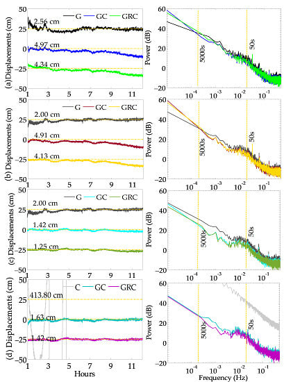
4.4. Assessment of Multi-GNSS PPP with Multipath Correction

As revealed by Geng et al. [16], the integration of GPS and GLONASS data led to a substantial reduction of the high-rate displacement noise by up to 40% compared to a GPS-only solution within European regions. In this section, the two major purposes investigated are presented. One shows the benefits from multi-GNSS in improving the precision of displacements; the other one concerns the question of whether the multi-GNSS data can suppress the effect of GEO periodic error. Four experiments numbered from (1) to (4) were designed, and the corresponding results of station GSWX in the east, north, and up direction are displayed in Figure 9a–d, Figure 10a–d, and Figure 11a–d, respectively.

Table 3. Data strategy of the designed four experiments.

Experiment	GRC with SF	GEO with SF	GEO Excluded
(1)	No	No	/
(2)	Yes	No	/
(3)	Yes	Yes	/
(4)	Yes	/	Yes

lists the data filtering strategy for the four experiments. Experiment (1) gives the results without sidereal filtering, whereas Experiments (2) to (4) present the sidereally filtered results. Note that the GEO observations are not filtered in Experiment (2), and they are excluded in Experiment (4).

From Figure 9a, it is observed that although the combined GPS/GLONASS/BDS (GRC) solution shows about 12.7% improvement compared to the GC combination, both of them are evidently inferior to the GPS-only solution. The fusion of GRC can effectively reduce most noise in contrast to the BDS solution without sidereal filtering, leading to a decline in the RMS values from 7.51, 3.50, and 11.38 cm to 4.34, 1.12, and 6.10 cm in the three components, respectively (see Figure 10; Figure 11), but there are still many fluctuations over the period of 5000 s remaining. After the sidereal filtering, a considerable reduction of 21.9% and 23.5% in terms of RMS can be found in the east and up components (see Figure 11), respectively, for GPS, whereas the SF approach may occasionally introduce undesirable ramps as shown in the north component around 6 to 7 h (see Figure 10). From a comparison between Figure 9a and Figure 9b, the application of SF on BDS IGSO and MEO observations can slightly reduce them by about 3.2 dB noise over periods from 50 s to 5000 s, but it fails in alleviating noise over longer periods. The RMS values for sidereally filtered GC and GRC solutions are comparable to those without sidereal filtering, which are 4.91 and 4.13 cm, respectively. Once the GEO observations are sidereally filtered (Experiment (3)), as delineated in Figure 9c, Figure 10c, and Figure 11c, the RMS values of the GRC solutions are reduced to 1.25, 0.81, and 3.79 cm from 4.34, 1.12, and 6.10 cm of Experiment (1), for the east, north, and up components, respectively, which are dramatic improvements of about 71.2%, 27.7%, and 37.9%, respectively. The PSDs across almost the entire frequency band decline substantially, especially for the longer periods where the PSDs decline on average by about 10.2 dB. Excluding the GEO satellites can improve the precision of GC and GRC solutions to some extent; however, it also increases the RMS values by 14.8% and 13.6% to 1.63 and 1.42 cm, respectively, compared with the sidereally filtered counterparts. Moreover, it seriously deteriorates the precision of the BDS-only PPP because of the poor geometry of the satellite constellation. Additionally, the sidereally filtered BDS-only solution (se Figure 7b) outperforms the unfiltered GPS solution in the east and up components (see Figure 9a and Figure 11a), but is slightly worse than the sidereally filtered GPS solution in the north and up components (see Figure 10b and Figure 11b).

4.5. A Case Study for the Mw6.3 Jiuzhaigou Earthquake

Two stations, SCJZ and GSZQ, close to the epicenter were selected to carry out the experiments, and the corresponding results are shown in Figure 12; Figure 13. The final coseismic displacements for these two stations were calculated using 15 days of GPS data before and 4 days after the event from [37]. For station SCJZ, although the data were interrupted after 48,032 s, the seismic waveforms were well recorded. The largest amplitudes of about 4 cm occurred in the north component for all the types of solutions. Compared with the north component for GPS, the seismic signal in the east displacement was indistinguishable from the noise, which might mislead preseismic analysis. In contrast, for BDS, the signal-to-noise ratio improved with the smaller fluctuations ahead of the event. The GRC solution without sidereal filtering was biased by about −1.30 cm in the east component, which was reduced by 89.2% to –0.14 cm after filtering. For station GSZQ, the largest fluctuation happened in the east component with a peak value of about –2.3 cm. The seismic waveforms embedded in the vertical direction were seemingly overwhelmed by high-level noise. Affected by the remaining systematic errors, some fluctuations of 2 to 3 cm spanning over several minutes could still be found in the east component for the BDS solutions. Because of the data interruption at station SCJZ, 2 h displacements of the sidereally filtered GRC solution before and after the arrival time of seismic waves were used to estimate the static offsets of station GSZQ, which were 1.9 mm and 5.4 mm with respect to the references 0.4 ± 1.2 mm and 3.6 ± 0.8 mm, in the east and north components, respectively. Overall, the superiority of the GRC solution with sidereal filtering over a single-system or unfiltered solution in alienating low-frequency errors on tens of seconds to minutes is clearly demonstrated.

5. Conclusions

For this study, the performance of multi-GNSS PPP, especially BDS PPP, in monitoring subtle deformation was investigated. The sidereal filtering approach was employed to mitigate the multipath in phase observations to improve the precision of PPP. The equations describing the relationship between phase residuals on different frequencies were rigorously derived, which could significantly reduce the complexity of multipath processing. A satellite-dependent periodic error term with an amplitude of up to ± 3 cm was found in the BDS GEO phase residuals, one of the main sources that limits the precision of BDS PPP. The results indicated that the systematic errors originated mainly from GEO, had periods longer than 2000 s, and could not be alleviated by the fusion of multi-GNSS, whereas the multipath errors from IGSO and MEO had periods from 50 to 5000 s. Traditionally, GEO observations are weighted lower to account for the imprecise orbit and clock products, but this also reduces the GEO’s contribution to the solution. The SF approach can effectively mitigate the periodic errors, thus improving the precision of the GEO phase to around 10 mm. Compared with the BDS-only PPP solutions without sidereal filtering, the one using the SF approach can effectively improve the positioning accuracy, with respect to the weekly averaged positioning solutions, by 75.2%, 42.8%, and 56.7% to 2.00, 2.23, and 5.58 cm in the east, north, and up components, respectively. It is comparable to that of GPS in the east component, and slightly worse in the north and up components. After applying sidereal filtering, the accuracy of the combined GPS, GLONASS, and BDS solution can also be improved by 71.2%, 27.7%, and 37.9% to 1.25, 0.81, and 3.79 cm in the three directions, respectively, compared to the unfiltered results.

References

1. Larson, K. GPS seismology. J. Geod. 2009, 83, 227–233. [Google Scholar] [CrossRef]
2. Bock, Y.; Melgar, D.; Crowell, B.W. Real-time strong-motion broadband displacements from collocated GPS and accelerometers. Bull. Seismol. Soc. Am. 2011, 101, 2904–2925. [Google Scholar] [CrossRef]
3. Crowell, B.W.; Bock, Y.; Melgar, D. Real-time inversion of GPS data for finite fault modeling and rapid hazard assessment. Geophys. Res. Lett. 2012, 39, L09305. [Google Scholar] [CrossRef]
4. Li, X.; Ge, M.; Guo, B.; Wickert, J.; Schuh, H. Temporal point positioning approach for real-time GNSS seismology using a single receiver. Geophys. Res. Lett. 2013, 40, 5677–5682. [Google Scholar] [CrossRef] [Green Version]
5. Larson, K.; Bodin, P.; Gomberg, J. Using 1-Hz GPS data to measure deformations caused by the Denali fault earthquake. Science 2003, 300, 1421–1424. [Google Scholar] [CrossRef] [PubMed]
6. Ruhl, C.J.; Melgar, D.; Chung, A.I.; Grapenthin, R.; Allen, R.M. Quantifying the Value of Real-Time Geodetic Constraints for Earthquake Early Warning Using a Global Seismic and Geodetic Data Set. J. Geophys. Res. 2019, 124, 3819–3837. [Google Scholar] [CrossRef]
7. Genrich, J.F.; Bock, Y. Instantaneous geodetic positioning with 10–50 Hz GPS measurements: Noise characteristics and implications for monitoring networks. J. Geophys. Res. 2006, 111, B03403. [Google Scholar] [CrossRef]
8. Zumberge, J.F.; Heflin, M.B.; Jefferson, D.C.; Watkins, M.M.; Webb, F.H. Precise point positioning for the efficient and robust analysis of GPS data from large networks. J. Geophys. Res. 1997, 102, 5005–5017. [Google Scholar] [CrossRef] [Green Version]
9. Collins, P.; Henton, J.; Mireault, Y.; Heroux, P.; Schmidt, M.; Dragert, H.; Bisnath, S. Precise point positioning for real-time determination of co-seismic crustal motion. In Proceedings of the ION GNSS 2009, Savannah, GA, USA, 22–25 September 2009; pp. 2479–2488. [Google Scholar]
10. Li, X.; Ge, M.; Zhang, X.; Zhang, Y.; Guo, B.; Wang, R.; Klotz, J.; Wickert, J. Real-time high-rate co-seismic displacement from ambiguity-fixed precise point positioning: Application to earthquake early warning. Geophys. Res. Lett. 2013, 40, 295–300. [Google Scholar] [CrossRef] [Green Version]
11. Li, X.; Ge, M.; Zhang, H.; Wickert, J. A method for improving uncalibrated phase delay estimation and ambiguity-fixing in real-time PPP. J. Geod. 2013, 87, 405–416. [Google Scholar] [CrossRef]
12. Li, X.; Ge, M.; Dai, X.; Ren, X.; Fritsche, M.; Wickert, J.; Schuh, H. Accuracy and reliability of multi-GNSS real-time precise positioning: GPS, GLONASS, BeiDou, and Galileo. J. Geod. 2015, 89, 607–635. [Google Scholar] [CrossRef]
13. Xu, P.; Shi, C.; Fang, R.; Liu, J.; Niu, X.; Zhang, Q.; Yanagidani, T. High-rate precise point positioning (PPP) to measure seismic wave motions: An experimental comparison of GPS PPP with inertial measurement units. J Geod. 2013, 87, 361–372. [Google Scholar] [CrossRef]
14. Zheng, K.; Zhang, X.; Li, X.; Li, P.; Sang, J.; Ma, T.; Schuh, H. Capturing coseismic displacement in real time with mixed single- and dual-frequency receivers: Application to the 2018 Mw7.9 Alaska earthquake. GPS Solut. 2019, 23, 9. [Google Scholar] [CrossRef]
15. Melgar, D.; Fan, W.; Riquelme, S.; Geng, J.; Liang, C.; Fuentes, M.; Vargas, G.; Allen, R.M.; Shearer, P.M.; Fielding, E.J. Slip segmentation and slow rupture to the trench during the 2015, Mw8.3 Illapel, Chile earthquake. Geophys. Res. Lett. 2016, 43, 961–966. [Google Scholar] [CrossRef]
16. Geng, J.; Jiang, P.; Liu, J. Integrating GPS with GLONASS for high-rate seismogeodesy. Geophys. Res. Lett. 2017, 44, 3139–3146. [Google Scholar] [CrossRef]
17. Cohen, C.; Parkinson, B. Mitigating multipath error in GPS-based attitude determination. In Proceedings of the Advances in the Astronautical Sciences, AAS Guidance and Control Conference, Keystone, CO, USA, 2–6 February 1991; pp. 74–78. [Google Scholar]
18. Dong, D.; Wang, M.; Chen, W.; Zeng, Z.; Song, L.; Zhang, Q.; Cai, M.; Cheng, Y.; Lv, J. Mitigation of multipath effect in GNSS short baseline positioning by the multipath hemispherical map. J. Geod. 2016, 90, 255–262. [Google Scholar] [CrossRef]
19. Choi, K.; Bilich, A.; Larson, K.; Axelrad, P. Modifed sidereal fltering: Implications for high-rate GPS positioning. Geophys. Res. Lett. 2004, 31. [Google Scholar] [CrossRef]
20. Zhang, Z.; Li, B.; Gao, Y.; Shen, Y. Real-time carrier phase multipath detection based on dual-frequency C/N0 data. GPS Solut. 2019, 23, 7. [Google Scholar] [CrossRef]
21. Fuhrmann, T.; Luo, X.; Knöpfler, A.; Mayer, M. Generating statistically robust multipath stacking maps using congruent cells. GPS Solut. 2015, 19, 83–92. [Google Scholar] [CrossRef]
22. Geng, J.; Pan, Y.; Li, X.; Guo, J.; Liu, J.; Chen, X.; Zhang, Y. Noise characteristics of high-rate multi-GNSS for subdaily crustal deformation monitoring. J. Geophys. Res. 2018, 123, 1987–2002. [Google Scholar] [CrossRef]
23. Yang, Y.; Li, J.; Wang, A.; Xu, J.; He, H.; Guo, H.; Shen, J.; Dai, X. Preliminary assessment of the navigation and positioning performance of BeiDou regional navigation satellite system. Sci. China Earth Sci. 2014, 57, 144–152. [Google Scholar] [CrossRef]
24. Shi, C.; Zhao, Q.; Hu, Z.; Liu, J. Precise relative positioning using real tracking data from COMPASS GEO and IGSO satellites. GPS Solut. 2013, 17, 103–119. [Google Scholar] [CrossRef]
25. Guo, F.; Zhang, X.; Wang, J. Timing group delay and differential code bias corrections for BeiDou positioning. J. Geod. 2015, 89, 427–445. [Google Scholar] [CrossRef]
26. Li, X.; Li, X.; Liu, G.; Feng, G.; Guo, F.; Yuan, Y.; Zhang, K. Spatial–temporal characteristic of BDS phase delays and PPP ambiguity resolution with GEO/IGSO/MEO satellites. GPS Solut. 2018, 22, 123. [Google Scholar] [CrossRef]
27. Kouba, J. A Guide to Using International GNSS Service (IGS) Products. Available online: http://kb.igs.org/hc/en-us/articles/201271873-A-Guide-to-Using-the-IGS-Products (accessed on 15 September 2019).
28. Li, P.; Zhang, X.; Ge, M.; Schuh, H. Three-frequency BDS precise point positioning ambiguity resolution based on raw observables. J. Geod. 2018, 92, 1357–1369. [Google Scholar] [CrossRef] [Green Version]
29. Deng, Z.; Zhao, Q.; Springer, T.; Prange, L.; Uhlemann, M. Orbit and clock determination-BeiDou. In Proceedings of the IGS workshop 2014, Pasadena, CA, USA, 23–27 June 2014. [Google Scholar]
30. Saastamoinen, J. Contributions to the theory of atmospheric refraction—Part II. Refraction corrections in satellite geodesy. Bull. Géod. 1973, 47, 13–34. [Google Scholar] [CrossRef]
31. Axelrad, P.; Larson, K.; Jones, B. Use of the correct satellite repeat period to characterize and reduce site-specific multipath errors. In Proceedings of the ION GNSS 18th International Technical Meeting of the Satellite Division, Long Beach, CA, USA, 13–16 September 2005; pp. 2638–2648. [Google Scholar]
32. Larson, K.; Bilich, A.; Axelrad, P. Improving the precision of high-rate GPS. J. Geophys. Res. 2007, 112, B05422. [Google Scholar] [CrossRef]
33. Agnew, D.C.; Larson, K.M. Finding the repeat times of the GPS constellation. GPS Solut. 2007, 11, 71–76. [Google Scholar] [CrossRef]
34. Shen, N.; Chen, L.; Liu, J.; Wang, L.; Tao, T.; Wu, D.; Chen, R. A Review of Global Navigation Satellite System (GNSS)-based Dynamic Monitoring Technologies for Structural Health Monitoring. Remote Sens. 2019, 11, 1001. [Google Scholar] [CrossRef]
35. Atkinson, K.E. An Introduction to Numerical Analysis; John Wiley & Sons: Hoboken, NJ, USA, 2018. [Google Scholar]
36. Ye, S.; Chen, D.; Liu, Y.; Jiang, P.; Tang, W.; Xia, P. Carrier phase multipath mitigation for BeiDou navigation satellite system. GPS Solut. 2015, 19, 545–557. [Google Scholar] [CrossRef]
37. Wang, Y.B.; Gan, W.J.; Chen, W.T.; You, X.Z.; Lian, W.P. Coseismic displacements of the 2017 Jiuzhaigou M7.0 earthquake observed by GNSS: Preliminary results. Chin. J. Geophys. 2018, 61, 161–170. [Google Scholar]
Figure 1. Distribution of the high-rate GNSS stations around the epicenter of the 2017 Mw 6.5 Jiuzhaigou earthquake event. The red star is the epicenter location.
Remotesensing 11 02232 g001
Figure 2. Correlation between the phase residuals from GPS (L1/L2), GLONASS (R1/R2), and BDS (B1/B2). The different color dots represent the residuals for different satellites. The regression lines, represented by the blue dashed lines, and the correlation coefficients (R) are also shown.
Remotesensing 11 02232 g002
Figure 3. Correlation between the residuals on frequencies B1 and B2 with different a priori precision of BDS GEO pseudo-range. The different color dots represent the residuals for different satellites. The regression lines, represented by the blue dashed lines, and the correlation coefficients (R) are also shown.
Remotesensing 11 02232 g003
Figure 4. The mean percentage errors of differences between the observed and projected phase residuals for L1/L2, R1/R2, and B1/B2.
Remotesensing 11 02232 g004
Figure 5. Carrier-phase residuals of C01 and C02 on two frequencies at station GMSD, CIBG, and JFNG from DOY 202 to 208, 2018. The opposite values of residuals on the second frequency are used.
Remotesensing 11 02232 g005
Figure 6. Carrier-phase residuals of C01 and C03 on two frequencies at stations DAE2, DAEJ, and GMSD from DOY 222 to 303, 2018. The opposite values of residuals on the second frequency are used.
Remotesensing 11 02232 g006
Figure 7. 12 h displacements (cm) with respect to weekly averaged positioning solutions for the east, north, and up components at station GSWX on DOY 219, 2018. The results with a priori phase precision of the GEO satellites of 15 mm, 10 mm, 6 mm, and 3 mm are depicted by black, blue, green, and purple lines, respectively, with the RMS statistics shown above the curves. Panel (a) presents the BDS PPP solution for which all BDS satellites except for the GEO satellites are sidereally filtered, while panel (b) presents solutions for which all the satellites are filtered. The lines have been shifted vertically to avoid overlap.
Remotesensing 11 02232 g007
Figure 8. Averaged power spectral density (PSD) (in dB) on a frequency band from 2 to 100,000 s over all five stations for the east, north, and up components on DOY 219, 2018. The sidereally filtered BDS solutions are exhibited by purple lines, while the solutions, for which all BDS satellites except for the GEO satellites are filtered, are exhibited by dark green lines.
Remotesensing 11 02232 g008
Figure 9. 12 h displacements (cm) with respect to daily solutions for the east component at station GSWX on DOY 219, 2018 and averaged power spectral density (PSD) (in dB) on a frequency band from 2 to 100,000 s over all 12 stations. (a) shows the solutions without sidereal filtering; (b) shows the solutions for which all satellites except for the GEO satellites are sidereally filtered; (c) shows the sidereally filtered solutions; (d) shows the sidereally filtered solutions excluding the GEO satellites from data processing. The yellow dashed-dotted horizontal lines denote the reference values.
Remotesensing 11 02232 g009
Figure 10. 12 h displacements (cm) with respect to daily solutions for the north component at station GSWX on DOY 219, 2018 and averaged power spectral density (PSD) (in dB) on a frequency band from 2 to 100,000 s over all 12 stations. (a) shows the solutions without multipath correction; (b) shows the solutions for which all satellites except for the GEO satellites are sidereally filtered; (c) shows the sidereally filtered solutions; (d) shows the sidereally filtered solutions excluding the GEO satellites from data processing. The yellow dashed-dotted horizontal lines denote the reference values.
Remotesensing 11 02232 g010
Figure 11. 12 h displacements (cm) with respect to daily solutions for the up component at station GSWX on DOY 219, 2018 and averaged power spectral density (PSD) (in dB) on a frequency band from 2 to 100,000 s over all 12 stations. (a) shows the solutions without sidereal filtering; (b) shows the solutions for which all satellites except for the GEO satellites are sidereally filtered; (c) shows the sidereally filtered solutions; (d) shows the sidereally filtered solutions excluding the GEO satellites from data processing. The yellow dashed-dotted horizontal lines denote the reference values.
Remotesensing 11 02232 g011
Figure 12. Displacements at station SCJZ during the Jiuzhaigou earthquake. The lines are shifted vertically to avoid overlap. The yellow dashed horizontal lines denote the mean of displacements. The black, blue, and purple lines refer to the sidereally filtered G, C, and GRC solutions, respectively, while the green lines refer to the GRC solution without sidereal filtering.
Remotesensing 11 02232 g012
Figure 13. Displacements at station GSZQ during the Jiuzhaigou earthquake. The lines are shifted vertically to avoid overlap. The yellow dashed horizontal lines denote the mean of displacements. The black, blue, and purple lines refer to the sidereally filtered G, C, and GRC solutions, respectively, while the green lines refer to the GRC solution without sidereal filtering.
Remotesensing 11 02232 g013