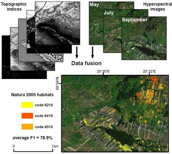
Multitemporal Hyperspectral Data Fusion with Topographic Indices—Improving Classification of Natura 2000 Grassland Habitats

Abstract

Accurately identifying Natura 2000 habitat areas with the support of remote sensing techniques is becoming increasingly feasible. Various data types and methods are used for this purpose, and the fusion of data from various sensors and temporal periods (terms) within the phenological cycle allows natural habitats to be precisely identified. This research was aimed at selecting optimal datasets to classify three grassland Natura 2000 habitats (codes 6210, 6410 and 6510) in the Ostoja Nidziańska Natura 2000 site in Poland based on hyperspectral imagery and botanical on-ground reference data acquired in three terms during one vegetative period in 2017 (May, July and September), as well as a digital terrain model (DTM) obtained by airborne laser scanning (ALS). The classifications were carried out using a random forest (RF) algorithm on minimum noise fraction (MNF) transform output bands obtained for single terms, as well as data fusion combining the topographic indices (TOPO) calculated from the DTM, multitemporal hyperspectral data, or a combination of the two. The classification accuracy statistics were analysed in various combinations based on the datasets and their terms of acquisition. Topographic indices improved the classification accuracy of habitats 6210 and 6410, with the greatest impact noted in increased classification accuracy of xerothermic grasslands. The best terms for identifying specific habitats were autumn for 6510 and summer for 6210 and 6410, while the best results overall were obtained by combining data from all terms. The highest obtained values of the F1 coefficient were 84.5% for habitat 6210, 83.2% for habitat 6410, and 69.9% for habitat 6510. Comparing the data fusion results for habitats 6210 and 6410, greater accuracy was obtained by adding topographic indices to multitemporal hyperspectral data, while for habitat 6510, greater accuracy was obtained by fusing only multitemporal hyperspectral data.

1. Introduction

Human activity causes constant transformation of the natural environment and affects biodiversity at all levels of its organization [1]. Being aware of the negative effects of this interference, human societies are attempting to counteract uncontrolled changes in the natural environment. The European network of Natura 2000 protected areas established under the Habitats Directive, sets out principles for protecting valuable habitats in Europe while identifying their threats [2]. Currently, the basic, widely used technique for identifying Natura 2000 habitats is on-ground measurement [3]. Based on the plant species composition, expert botanists categorise patches of given plant communities as relevant Natura 2000 habitats. The largest problems with such studies are that they are subjective, time-consuming for large areas and cannot penetrate inaccessible areas, such as swamps [4] and steep slopes [5]. In contrast to on-ground methods, remote sensing methods provide significant savings in the time and human resources needed to identify natural vegetation with suitable precision. As a consequence, they enable changes in extent or state of preservation to be determined [4]. Fusing data obtained from various sensors (e.g., spectral and airborne laser scanning (ALS) data) with ground reference data leads to improved classification quality compared to classification results from single-sensor data [6]. When using multiple data sources and types, an important consideration is the principled selection of data processing and analysis solutions specific to the purpose, in order to preserve one of the main advantages of using remote sensing methods: saving time [7].

Previous studies reported in the literature present different approaches to the classification of plant communities or Natura 2000 habitats using remote sensing data. Studies often use high spatial resolution data (a feature that is particularly relevant in object-based methods) [8,9] and high spectral resolution data (of importance in pixel-level classification) [10,11]. Various algorithms are used in classifying plant communities. These methods differ in the type of learning, assumptions about the number of training polygons, and input data types. The methods that are most commonly used and which provide the best results include: (a) machine learning algorithms, such as support vector machines (SVM) [12,13,14,15] and random forest (RF) [4,16,17]; and (b) methods that allow a probability threshold to be determined as to whether a given area belongs to a particular class, including linear discriminant analysis (LDA) [11] and spectral mixture analysis [8,10,18]. Authors who use machine learning methods like SVM or RF point out that they can achieve high accuracy [5,12,14], with greater simplicity and a somewhat briefer classification process than similar accuracy achieving neural networks [19,20]. The key advantage of using machine learning algorithms in image classification is that they cope with multidimensional data in ways that are acceptable statistically, which is why they are recommended as effective for use with hyperspectral data [21]. In the case of an iterative machine learning classification process, the speed of model training is significant, but is much shorter for the RF method than for other machine learning algorithms [22]. In the case of Natura 2000 habitats, several of which can often be identified in a single area, authors more often use the RF algorithm compared to other machine learning algorithms [4,16,17].

Vegetation mapping most often uses data obtained by sensors registering electromagnetic spectra in the visible, near- and mid-infrared ranges, both multispectral [23,24], and hyperspectral [5,10,25]. Authors who have sought to classify Natura 2000 habitat have also capitalized on ALS [4] fused with multispectral data [23] or hyperspectral data [9,26]. Products derived from ALS, such as those related to the vertical structure of vegetation [27], canopy height models (CHM) [9], topographic indices such as the topographic position index [23], and values calculated based on a digital terrain model (DTM; e.g., mean, maximum, standard deviation [9]), are commonly used in studies concerning habitat mapping. The selection of particular data products and derivatives depends on the specificity of a given habitat; in the case of vertical structure rasters and CHM, it is important that the species comprising the habitat in question differ in structure or height, while topographic indices present habitat features describing location, wetness, potential availability of solar energy and the like. This is particularly significant in topographically diverse terrain.

When using data fusion techniques, it is important to know the significance of individual input variables (layers) in the classification process [23]. One important factor for classifying plant communities is the term(s) in the meaning of temporal period of acquisition of remote sensing data. The literature is dominated by studies of plant communities and Natura 2000 habitat identification using remote sensing data obtained in a single term [10,16,28]. This is often the only approach possible due to the lack of appropriate multitemporal datasets. In such cases, remote sensing data may not be acquired at the optimum time for vegetation to be classified, which is indicated as the cause of lower-than-expected accuracy [4]. While less common, the literature also offers examples of the classification of plant communities using multitemporal datasets. In these cases, data from multiple phenological periods has proven to be extremely value in properly classifying vegetation communities [24,29,30]. Capitalizing on information from different terms can provide more reliable results, in part due to the possibility of capturing specific vegetative features in different phonological phases, such as flowering, fruiting and autumnal coloration.

The use of multitemporal data for vegetation analysis often falls within the domain of moderate resolution satellite data, such as MODIS (250–500 m) [31], Landsat (30 m) [32] and Sentinel-2 (10–20 m) [33] optical data. Authors using finer resolutions for vegetation classification have applied multitemporal data fusion to multispectral 5 m RapidEye data [24,29] and fusion of multitemporal data with data from active sensors, such as radar [34]. Many works present greater possibilities for detailed vegetation classification using hyperspectral data as compared to multispectral, due to the continuous nature of spectra [15,35,36]. There are currently no works in the scientific literature presenting the use of multitemporal hyperspectral data in natural vegetation classification of Natura 2000 habitats. Additionally, fused with ALS data, multitemporal hyperspectral data may be even more valuable in precisely identifying habitats. As underlined by the main objective of the data fusion approach, it leads to provide more accurate analytical outcome [37], and studies utilizing data fusion have shown increased accuracy related to increased numbers of variables used [9]. However, due to the high cost of aerial data acquisition, in order to optimize the classification process, it is important to know which datasets are the most relevant to the task at hand.

Remote sensing imaging is often accompanied by on-ground measurements to collect reference data [12,26,38]. In the absence of such field work, information from existing maps is used, in which case attention should be paid to their scale and degree of temporal coincidence. The use of reference data acquired in the field at the moment of remote sensing data acquisition is of particular importance in studies of vegetation, which is variable over the growing season, due to both phenology and land use. In multitemporal analysis, the key is to have multitemporal on-ground reference samples and reliable multitemporal image data representing all classes, the inter-relationship between them, and spatial and temporal variability. However, in real-world application this can be a challenging task [39].

This study aims to assess the impact on accuracy of the classification of three Natura 2000 habitats (semi-natural dry grasslands and scrubland facies on calcareous substrates, code 6210; Molinia meadows on calcareous, peaty or clayey silt-laden soils, code 6410; and lowland hay meadows, code 6510) and (a) aerial hyperspectral data and their fusion with topographic indices, and (b) the fusion of multitemporal hyperspectral data acquired in three different terms of the phenological period and their fusion with topographic indices. More specifically, our research aims to select the best dataset for classifying each habitat, focusing on optimizing this selection, where optimization is viewed as the compromise between high accuracy and time- and cost-effectiveness of data acquisition and processing. To realize these purposes, the following data were used: aerial hyperspectral data registered in the visible, near infrared (VNIR) and shortwave infrared (SWIR) ranges from measurement campaigns conducted in spring, summer and autumn of 2017; botanical on-ground reference data collected in the field synchronously with the aerial campaigns; and a DTM obtained in spring 2017 using ALS. Aerial data transformed into minimum noise fraction (MNF) bands and topographic indices were used to develop 14 classification datasets, in the following combinations: (a) MNF data from individual terms paired with topographic indices, (b) multitemporal fusion of MNF bands from more than one acquisition term, and (c) multitemporal fusion of MNF bands from more than one acquisition term paired with topographic indices. These sets were subjected to random forest iterative classification and validation using training data randomly sampled from botanical reference polygons. To the best of our knowledge, this is the first study to classify Natura 2000 grassland habitats using multitemporal hyperspectral data and, as a consequence, the first study fusing them with topographic indices.

2. Materials and Methods

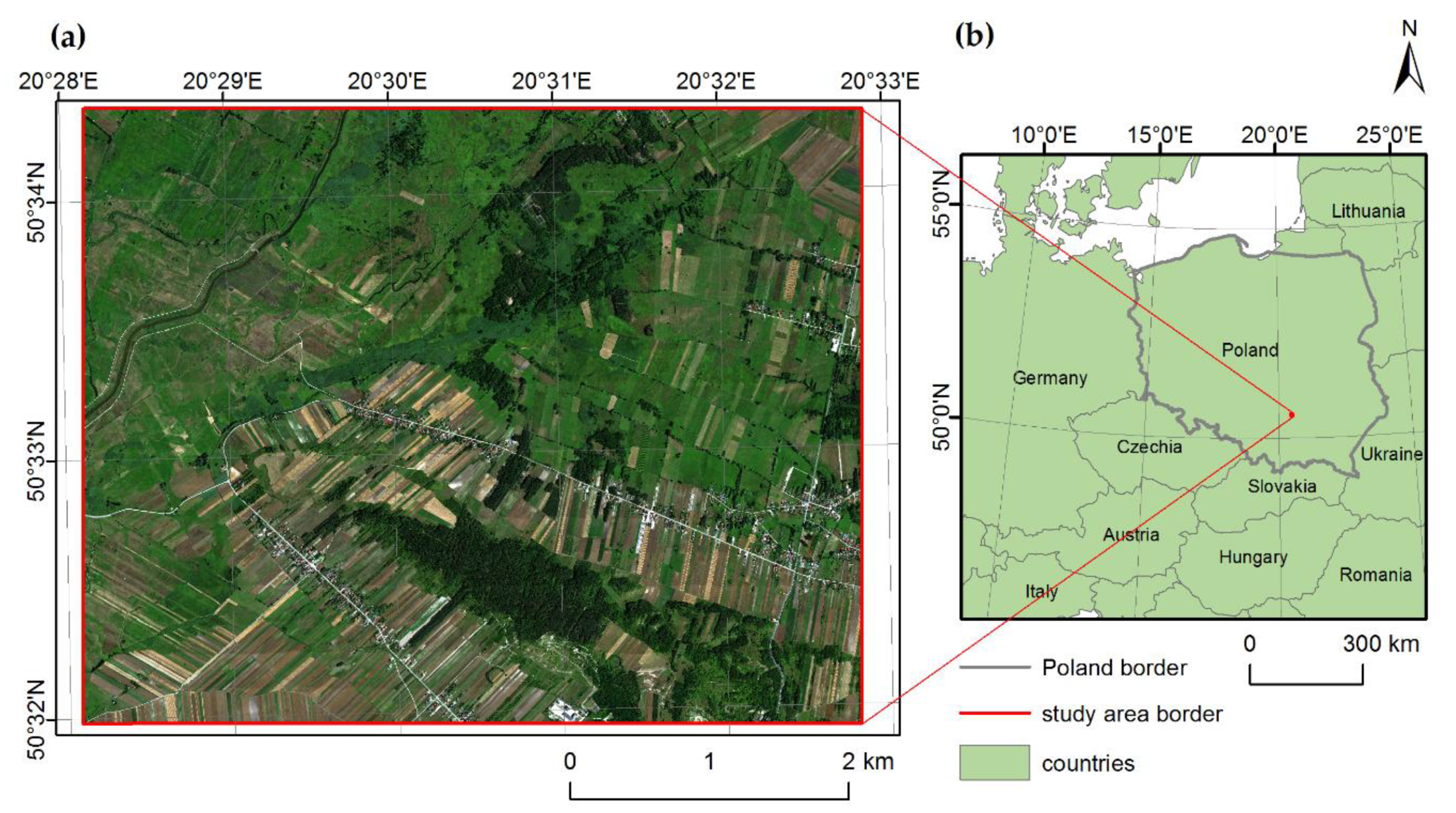
2.1. Study Area and Focus

The research area, approximately 24.6 km², is located in southern Poland, in the south of the Świętokrzyskie voivodeship (Figure 1). Most of the area (about 19.3 km²) is located within a special area of conservation (SAC) – Ostoja Nidziańska (code: PLH260003), which is protected as part of the Natura 2000 network. The vegetation in the area is semi-natural due to long-term agricultural and pastoral exploitation.

We analysed three Natura 2000 habitats (Figure 2): semi-natural dry grasslands and scrubland facies on calcareous substrates (Festuco-Brometalia, 6210); Molinia meadows on calcareous, peaty or clayey silt-laden soils (Molinion caeruleae, 6410); and lowland hay meadows (Alopecurus pratensis, Sanguisorba officinalis, 6510) [40]. To function optimally, these habitats should be extensively used by humans. The intensification or absence of agricultural use may cause the character of these habitats to be transformed or degraded. These habitats are characterized by high species diversity, and in most cases their patches have irregular boundaries which are not spatially cohesive within the borders of parcels.

Natura 2000 habitat 6210 most often occurs on calcium carbonate slopes in river valleys and on outcrops of limestone, usually in places with long sunshine duration on south-facing slopes. The habitat is diverse in terms of dominant species; patches can be dominated by, among others: Brachypodium pinnatum, Peucedanum cervaria, Carex humilis and Inula ensifolia. The plant composition of these semi-natural dry grasslands and scrubland facies is the result of extensive livestock grazing and mowing, and occasional burning. In the event that systematic use of these grasslands ceases, there is the threat that habitat 6210 will be transformed into thickets, as a result of secondary succession, and then into forest. There is also a threat to semi-natural dry grasslands and scrubland stemming from abandonment of agricultural use and artificial afforestation. The basic tasks of biodiversity conservation in habitat 6210 are to cut down trees and shrubs covering areas of grasslands, and to maintain or restore extensive forms of use (grazing, mowing, controlled burning).

Habitat 6410 is created by extensive human activity. The habitat requires mowing once a year or less, at the turn of August–September. In the research area in 2017, the patches that predominated still had not been mown by the third measurement campaign. Molinia meadows grow mainly in forest clearings with a broad spectrum of soils ranging from poor acidic to fertile alkaline [41]. Vegetation species diversity depends largely on water depth in a given habitat, which results in species with diverse habitat requirements occurring within one habitat. Typical species include Galium boreale and Molinia caerulea. The management of areas of variable moisture—on which habitat 6410 develops—as agricultural grasslands causes Molinia meadows to disappear from their area of natural occurrence. The succession resulting from the abandonment of extensive use of habitats of this type in favour of more valuable grassland threatens the existing sites of Molinia meadows.

Habitat 6510 is largely found in ameliorated sections of river valleys, on flats along floodplains or on gentle slopes of wide valleys. In terms of water–soil relations and thermal conditions, individual patches of this habitat are highly diverse. The character of each habitat 6510 also depends on the intensity of human activity (grazing, mowing). In the study area in 2017, the majority of the habitat patches were exploited by mowing twice a year. The species occurring in the patches of this habitat depend on the geographical and climatic conditions, and on the type and extent of human use. The predominant species are mainly grasses, such as: Festuca rubra, Avenula pubescens, Deschampsia caespitosa, Poa pratensis and Arrhenatherum elatius. Due to the anthropogenic nature of the creation of lowland hay meadows, their preservation in optimal condition depends on the perpetuation of regular, low- or medium-intensity mowing and fertilisation.

2.2. Remote Sensing Data

Aerial data were obtained using a combination of instruments on a Habitats Airborne Remote Sensing (HabitARS) multi-sensor platform [17] in 2017 in three campaigns—spring (18 May, C1), summer (30 July, C2) and autumn (27 September, C3). The data were obtained using an aerial hyperspectral scanner, VNIR sensor, SWIR sensor, laser scanner, and a red-green-blue RGB photogrammetric camera. Detailed characteristics of the HabitARS platform and sensors and its sensors and parameters, as well as the scope of processing of obtained data, are described in articles by Marcinkowska-Ochtyra et al. [30] and Sławik et al. [17]. The effectiveness of the methods used to prepare the hyperspectral data was verified in articles by Nimbalkar et al. [42] and Sabat-Tomala et al. [43].

2.2.1. Hyperspectral Data

Aerial hyperspectral images were registered using two HySpex scanners (Norsk Elektro Optikk, Oslo, Norway): a VNIR-1800 (range 400–1.000 nm, 182 bands, spectral sampling 3.26 nm, spatial resolution 0.5 m) and an SWIR-384 (range 950–2500 nm, 288 bands, spectral sampling 5.45 nm, spatial resolution 1 m). The combined data from both scanners were subjected to the necessary procedures [17]: radiometric calibration, parametric geometric correction in PARGE software (ReSe—Remote Sensing Applications, Wil, Switzerland) [44], and atmospheric correction using the MODTRAN5 radiative transfer model in the ATCOR4 software (ReSe Applications GmbH, Wil, Switzerland) [45]. The processed spectra of 1-m spatial resolution were mosaicked. Having so many spectral bands, it was essential to perform dimensionality reduction. In order to eliminate noise and select the most informative bands, the hyperspectral mosaics were subjected to an MNF transformation [46] using ENVI 5.5 software (Harris Geospatial Solutions, Broomfield, CO, USA). Covariance matrices and noise correlations on the original mosaics were used to calculate eigenvalues. Based on the highest eigenvalues (more than 1), 30 MNF bands were initially selected, and then, based on visual interpretation (on account of noticeable noise and artefacts surrounding mosaicking lines), 15 individual MNF bands were finally selected. These procedures were repeated for all data from campaigns C1, C2 and C3.

2.2.2. Airborne Laser Scanning Data

Airborne laser scanning data were registered as a point cloud with a density of 7 point/m² using a Riegl LMS-Q 680i laser scanner (Integrated Geospatial Innovations, Kreuztal, Germany). ALS data processing included orientation, decomposition and classification of the point cloud. Orientation was carried out with accuracy assessed at the level of 1S = 0.010 cm and the point cloud from full-waveform decomposition was classified into noise, ground, and vegetation classes automatically with further manual validation [5,17] (developed features were excluded from our analysis through masking). Processed ALS data was used to generate the DTM. Due to the specific nature of our study site (see Section 2.1), we decided to derive layers from the ALS associated with topographic features that might affect habitat conditions. It was assumed that the terrain, which conditions the moisture and, thus, the potential species composition, might be helpful in identifying the examined habitats. Of the three dates on which ALS data were obtained, the springtime data had the highest degree of plant cover penetration by the laser beam, due to plant growth being in its earliest stage. As a result, the measurement of the site’s true elevation was considered the most accurate in this season. Based on the DTM, five topographic indices were calculated (TOPO) [17] with a spatial resolution of 1 m (

Table 1. Topographic indices.

Application	Product	Acronym	Reference
Morphometric analysis	Multiresolution Index of Valley Bottom Flatness	MRVBF	[48]
	Multiresolution Index of the Ridge Top Flatness	MRRTF
	Topographic Position Index	TPI	[49,50]
Hydrologic analysis	Topographic Wetness Index	TWI	[51,52,53]
	Modified Catchment Area	MCA	[53,54]

), using SAGA 2.3.2. software [47] (System for Automated Geoscientific Analyses, Hamburg, Germany).

2.2.3. Data Fusion

In order to investigate the impact of data fusion strategies on classification accuracy, we combined our three sets of MNF layers and our five topographic layers in 10 unique ways. We subjected each of these 10 input datasets to RF classification (

Table 2. Datasets subjected to random forest (C1, C2, C3—campaign number, MNF—minimum noise fraction, TOPO—topographic indices).

Dataset Name	MNF			TOPO
	Spring (C1)	Summer (C2)	Autumn (C3)
C1_MNF	X
C2_MNF		X
C3_MNF			X
C1_MNF+TOPO	X			X
C2_MNF+TOPO		X		X
C3_MNF+TOPO			X	X
C1_C2_MNF7	X	X
C1_C3_MNF	X		X
C2_C3_MNF		X	X
C1_C2_C3_MNF	X	X	X
C1_C2_MNF+TOPO	X	X		X
C1_C3+TOPO	X		X	X
C2_C3+TOPO		X	X	X
C1_C2_C3+TOPO	X	X	X	X

). Our analysis relied on three core assumptions. First was that for the fusion of hyperspectral and topographic data, the MNF layer was the primary determinant of the classification, and the TOPO layer played a complementary role (Table 2). Second assumption was that for the multitemporal fusion of hyperspectral data the C1, C2, and C3 campaigns were all equally important, and so each was combined with the others, and all were combined together (Table 2). Third assumption was that the application of both types of fusion (MNF + TOPO and multitemporal MNF fusion) will improve the accuracy. Based on this, we combined all the data, in order to compare the results of all data fusion set to MNF + TOPO and multitemporal MNF fusion. This step enabled us to select optimal dataset.

2.3. Reference Data

While aerial remote sensing data was being acquired, ground-based measurements were conducted in parallel, during which training and validation sets were collected. The measurements were carried out within seven days of the aerial data acquisition date in order to obtain reference data with maximal fidelity to the true state of the vegetation as represented in the remote sensing data. Reference polygons, each with a 3 m buffer, were collected for three Natura 2000 habitats (6210, 6410 and 6510) and for other communities or plant complexes, collectively referred to as the “background” class. Botanists used Global Navigation Satellite System (GNSS) Spectra Precision GPS MobileMapper 120 receivers (Spectra Geospatial, Westminster, CA, USA) with real-time differential correction and a measurement accuracy from 1.0 m to 0.2 m. During the work, information was collected on land cover types in a given polygon, date of measurement, and the polygon’s dominant species. Polygons were validated using data from all three campaigns, such that polygons that were in shade or recently mown in any campaign were removed from the reference dataset. A single reference dataset was prepared for evaluating all of our classifications. It contained polygonal features gathered across all campaigns, while ensuring there was no duplication or confounding effects from inter-campaign land-use change (

Table 3. Number of polygons collected for each campaign and in combined multitemporal reference dataset for each habitat and associated background (C1, C2, C3—campaign number).

Class	No. of Polygons
	C1	C2	C3	Combined into Multitemporal Set
6210	323	339	321	347
6410	262	229	232	292
6510	250	236	250	267
background	892	868	896	954

).

In order to exclude areas which did not belong to the habitat of interest or other non-forest natural vegetation classes, we excluded forest and water from our analysis by masking representative areas. For forest masking, we applied a threshold of 2 m in height as derived from the CHM. For water masking, we used the near-infrared band (844 nm) of our hyperspectral mosaic. Additionally, we masked buildings within parcels using orthophoto interpretation and local land parcels database.

2.4. Classification and Iterative Accuracy Assessment

All ten datasets were classified using the random forest algorithm with the ‘randomForest’ package [55] of R software [56]. In the RF algorithm, training data in the form of class signature pixel values are used as the basis for determining the rules by which all pixels are allocated to specific classes according to the majority vote across all decision trees [57]. Random selection of the training sample and rules of split enables algorithm to be robust to classification model overfitting [58]. For each classification we used 500 trees (ntree parameter). This selection was made based on testing the stability of out-of-bag (OOB) error rate (we tested 100-1000 trees in steps of 100). The number of variables to be selected for the split (mtry parameter) was set to the square root of the number of input variables for each dataset individually [59]. In RF, the variable importance measure is useful for identifying the most relevant explanatory variables, hence it was applied to this work. For the best iterations obtained across all data fusion sets (multitemporal with TOPO fusion), we present variable importance plots showing the top 10 most influential variables (Supplementary Materials, Figures S1–S3).

To ensure that each observation in our reference dataset contributed to the analysis, iterative classification and validation of results was performed 100 times using a bootstrap procedure [60,61]. The reference data were split into 50/50 proportions of training and validation sets using per-class stratified random sampling, assigning equal numbers of polygons to each class for model training and validation [62,63]. This approach ensured 100 unique training and testing datasets, which (a) helped reduce bias associated with any particular 50/50 split, and (b) enabled us to evaluate the variability and stability of classification accuracy [61]. We applied an identical workflow to each of our 14 input datasets (Table 2), leading us to implement the RF classifier a total of 1400 times.

For all classifications, accuracy was assessed using the following measures: overall accuracy (OA; the sum of correctly classified pixels divided by the total number of classified pixels) [64] and the F1 coefficient for individual classes, which is the harmonic mean of producer’s accuracy (PA; the number of correctly classified pixels divided by the total number of pixels in the reference class) and user’s accuracy (UA; the number of correctly classified pixels divided by the number of pixels classified into the class) [65]: F1 = 2 × (UA + PA) / (UA × PA). The statistical significance of differences in OA and F1 accuracy obtained for each dataset was assessed using the nonparametric U Mann–Whitney Wilcoxon test at α = 0.05. The classification accuracies obtained during the 100 iterations allowed accuracy statistics to be presented and interpreted as boxplots of their distributions. In order to avoid the influence of outliers, we adopted the median accuracies from each set of 100 iterations as our best-fit values [66]. This allowed the results of particular combinations to be compared with greater certainty than using single values (e.g., maxima) obtained using a one-time random selection of a set of training and validation polygons. In order to present all classified habitats on one map, the classification image of the iteration with the highest mean of three median F1 values for the three habitats was selected, for which commission and omission errors were also calculated.

3. Results

All obtained results in the form of OA and F1 accuracy are presented in Figure 3 and Figure 4, and

Table 4. The results of all classifications (C1, C2, C3—campaign number, MNF—minimum noise fraction, TOPO – topographic indices).

Dataset	OA [%]	Median F1 [%] for Natura 2000 Habitat			Mean F1 for 3 Natura 2000 Habitats [%]
		6210	6410	6510
C1_MNF	70.6	74.0	68.9	51.7	64.9
C2_MNF	75.1	79.5	75.2	59.5	71.4
C3_MNF	75.5	78.3	75.0	61.1	71.5
C1_MNF+TOPO	74.1	79.5	73.4	55.8	69.6
C2_MNF+TOPO	76.9	82.3	77.7	60.5	73.5
C3_MNF+TOPO	77.6	83.1	79.6	61.6	74.8
C1_C2_MNF	78.6	81.6	80.1	65.5	75.7
C2_C3_MNF	80.0	82.9	80.8	68.0	77.2
C1_C3_MNF	78.5	81.4	80.1	64.3	75.3
C1_C2_C3_MNF	81.0	83.7	82.4	69.9	78.7
C1_C2_MNF+TOPO	79.5	83.7	80.9	65.8	76.8
C2_C3_MNF+TOPO	79.8	83.1	81.2	67.9	77.4
C1_C3_MNF+TOPO	79.4	83.6	82.0	64.8	76.8
C1_C2_C3_MNF+TOPO	81.1	84.5	83.2	68.9	78.9

. The descriptions of each result in relation to the dataset used are presented in Section 3.1, Section 3.2 and Section 3.3. Single date MNF + TOPO and multitemporal MNF classification results were first analysed in comparison to a reference set of one-date MNF, showing increased accuracy with the application of each fusion. In Section 3.4 we compare the results achieved with all datasets to the multitemporal MNF + TOPO set, which we believed, a priori, would yield the highest accuracy. Based on the differences between these datasets, we indicate the optimal variant for each habitat classification. Classification image most reliably presenting the distribution of habitats in the study area has been chosen on the basis of highest mean F1 coefficient value of three habitats.

3.1. Single Date Hyperspectral Data Classification

As a result of the classification of MNF data from individual terms (C1_MNF, C2_MNF, C3_MNF), 300 classification statistics were obtained—100 for each of the three terms. The results were analysed for overall classification accuracy (Figure 3). Medians of overall accuracy were in the range 70.6–75.5%. The lowest OA was achieved using the MNF set from campaign C1, and the highest using campaign C3. Differences between the minimum and maximum values for each campaign were similar, and ranged from 3.4% (C3_MNF) to 5.1% (C1_MNF).

Habitat 6210 had the highest median F1 coefficient, at 79.5% for the C2_MNF set, with the C3_MNF set not far behind (78.3%), while the lowest was for the C1_MNF set, at 71.7% (Figure 4a). For the median F1 coefficient for habitat 6410, the variance was 9.7% (in the range of 68.9% for C1_MNF to 75.2% for C2_MNF, Figure 4b). The second highest F1 value was for the C3 campaign (75.0%). The values of the F1 coefficient for habitat 6510 ranged from a minimum of 51.7% (C1_MNF) to a maximum of 61.1% (C3_MNF, Figure 4c).

3.2. Hyperspectral and Topographic Data Fusion Classification

As a result of classifying data using the fused MNF + TOPO from individual terms (C1_MNF + TOPO, C2_MNF + TOPO, C3_MNF + TOPO), 300 sets of classification statistics were also obtained, 100 for each of the three datasets. An analysis of the overall classification accuracy (Figure 3) revealed higher median values than for MNF bands alone, and these ranged from 74.1% to 77.6%. Similarly, the lowest OA was achieved for the set using MNF bands from campaign C1, and the highest for the set with campaign C3 MNF bands. Differences between the maximum and minimum values among those obtained from the 100 iterations were similar for each of the campaigns, and amounted to 4.7% for the autumn campaign, 4.9% for the spring campaign and 5.5% for the summer campaign. The greatest improvement over OA for MNF bands alone was obtained for the C1 campaign (3.5%), and the lowest gain in accuracy was observed for the C2 campaign (1.8%).

Analysing the F1 values, the highest median for habitat 6210 was observed for the set C3_MNF+TOPO (83.1%), and the lowest for C1_MNF + TOPO (79.5%, Figure 4a). For this habitat, the improvement over F1 medians for MNF bands alone was greatest, and amounted to 4.9% and 5.5%, respectively. For the C2 campaign, the fused set of MNF and topographic indices gave an accuracy of 82.3%, which was 2.8% higher than for MNF alone. For habitat 6410, the highest median F1 value was also obtained for the C3_MNF+TOPO set, and this value was as much as 8.9% higher than the lowest, which was again obtained for the C1_MNF+TOPO set (Figure 4b). These values were also higher than those obtained on the MNF bands alone, by 4.6% and 4.5%, respectively. For the C2 campaign, the improvement over the set consisting of MNF bands alone was small (2.5%). For habitat 6510 the F1 coefficient values for the C2 and C3 campaigns were very similar, with the autumn campaign (61.6%) slightly higher than the summer one (60.5%; Figure 4c). The lowest value, as for the other habitats, was obtained for the MNF + TOPO set from the spring campaign (55.8%). The fusion of MNF bands with topographic indices brought improvement in accuracy of habitat 6510 F1 values at 4.1%, 1.0% and 0.5% over MNF bands only for spring, summer and autumn sets, respectively.

3.3. Multitemporal Hyperspectral Data Fusion Classification

Using the fused multitemporal data, 400 classification statistics were obtained. Among the fused multitemporal hyperspectral datasets, the highest median overall classification accuracy was achieved for the set consisting of a combination of all hyperspectral data-acquisition terms C1_C2_C3_MNF, at 81.0% (Figure 3). The second-highest median OA was for the C2_C3_MNF set, at 80.0%. The set with the lowest median OA was the combined data from the spring and autumn campaigns (78.5%). The differences between minimum and maximum OA values of individual sets were reasonably stable between 3.6% for C1_C2_MNF and 4.1% for C2_C3_MNF. Median overall accuracies for data fusion consisting of more than one term was higher than the results of OA for single terms (the difference between the highest OAs obtained for C3_MNF and C1_C2_C3_MNF was 5.5% and between the lowest OAs obtained for C1_MNF and C1_C3_MNF was 7.9%).

For each habitat, the highest median accuracy of the F1 coefficient was obtained from the C1_C2_C3_MNF dataset (Figure 4). For habitat 6210, the median F1 values ranged from 83.7% (C1_C2_C3_MNF) to 81.4% (C1_C3_MNF, Figure 4a). These were, respectively, 5.4% and 7.4%, higher than the values obtained for the sets with the highest and lowest median F1 for MNF bands alone. The combination of MNF bands from summer and autumn terms provided the second highest median accuracy (82.9%). For habitat 6410, the highest median F1 was 82.4% (C1_C2_C3_MNF), and a slightly lower accuracy of 80.8% was obtained for the C2_C3_MNF dataset (Figure 4b). They were, respectively, 7.2% and 5.6% higher than the best single-term set (C3_MNF). Slightly lower multitemporal fusion results for this habitat were observed for the C1_C2_MNF and C1_C3_MNF sets (80.1%) which was 11.2% higher than the lowest value obtained for the C1_MNF set. The median F1 for class 6510 ranged from 64.3% (C1_C3_MNF) to 69.9% (C1_C2_C3_MNF, Figure 4c). The second-best multitemporal fusion set combined data from summer and autumn (68.0%). As with the previous habitats, accuracy obtained for the multitemporal fusion data was higher than that obtained for single terms. The differences between the best and worst sets for habitat 6510 were 8.8% and 12.6%, respectively.

3.4. Multitemporal Hyperspectral and Topographic Data Fusion Classification

Another 400 sets of classification statistics were obtained for the fused multitemporal hyperspectral data and topographic indices. The highest median OA from 100 iterations was measured for the C1_C2_C3_MNF + TOPO set (81.0%; Figure 3). The difference in OA between the three remaining multitemporal MNF + TOPO sets was just 0.4% (79.3–79.7%). Amplitudes of OA among iterations of the sets were in the range of 3.5–4.2%.

Each of the highest median F1 values for all three habitats was achieved with the C1_C2_C3_MNF + TOPO dataset (Figure 4). The best result for habitat 6210 (84.5%) was 0.7% better than the second best result (C1_C2_MNF+TOPO) and 5% higher than the highest F1 achieved with the respective one-data MNF dataset (Figure 4a). For habitat 6410, the best result of 83.2% was followed by 82.0% (C1_C3_MNF + TOPO), with the lowest accuracy of 80.9% was obtained using the C1_C2_MNF + TOPO dataset (Figure 4b). The maximum F1 accuracy achieved for habitat 6410 using all available data (83.2%) was 8.0% better than the best result achieved with one-date MNF bands. The results of 6510 habitat classification were in the range of 64.7% (C1_C3_MNF + TOPO) and 68.9%, with the second best accuracy (67.9%) captured by the C2_C3_MNF + TOPO dataset (Figure 4c). The difference between the highest F1 values for habitat 6510 achieved with one-date MNF bands and multitemporal MNF + TOPO data was 7.8%.

3.5. Comparison of Results for All Datasets

To select a single best input dataset for use in classifying all three of our target habitats, we compared median OA values, median F1 coefficients calculated for habitats (Figure 3 and Figure 4, Table 4), statistical significance of differences in accuracy statistics among datasets (

Table 5. Datasets for which F1 accuracy differences were not significant statistically using U Mann-Whitney Wilcoxon test (α = 0.05; C1, C2, C3—campaign number, MNF—Minimum Noise Fraction, TOPO – topographic indices, a—habitat 6210, b—habitat 6410, c—habitat 6510).

C1_MNF

abc

C2_MNF

abc

b

a

C3_MNF

b

abc

c

c

C1_MNF+TOPO

a

abc

C2_MNF+TOPO

c

abc

C3_MNF+TOPO

c

abc

a

b

a

C1_C2_MNF

abc

ab

c

C2_C3_MNF

a

abc

b

abc

C1_C3_MNF

b

ab

abc

c

C1_C2_C3_MNF

abc

a

a

c

C1_C2_MNF+TOPO

c

b

a

abc

b

a

C2_C3_MNF+TOPO

a

abc

b

abc

C1_C3_MNF+TOPO

c

a

a

abc

C1_C2_C3_MNF+TOPO

c

abc

C1_MNF

C2_MNF

C3_MNF

C1_MNF+TOPO

C2_MNF+TOPO

C3_MNF+TOPO

C1_C2_MNF

C2_C3_MNF

C1_C3_MNF

C1_C2_C3_MNF

C1_C2_MNF+TOPO

C2_C3_MNF+TOPO

C1_C3_MNF+TOPO

C1_C2_C3_MNF+TOPO

, Table S1), as well as means of the three median F1 coefficients (Table 4).

The largest difference in median OA among all datasets (Figure 3) was noted between C1_C2_C3_MNF + TOPO (best) and C1_MNF (worst)—over 10%. Disparities in median F1 coefficient values for habitats (Figure 4) were also the most significant between aforementioned datasets—approximately 8% for 6210 and 6410 habitats and 17% for 6510 habitat. This habitat (6510) is a particular example of higher F1 accuracy obtained for datasets other than C1_C2_C3_MNF + TOPO, which we treated as a reference; for C1_C2_C3_MNF, the median accuracy increased by 1% (Table 4) and the difference was not significant statistically (Table 5). It confirms that for classification of habitat 6510, fusion of hyperspectral and TOPO data does not improve classification accuracy, but the dataset consisting of all, or even only summer and autumn, sets could be enough. The C3 MNF + TOPO dataset is the only example of a difference smaller than 2% in decreased F1 accuracy when using fusion without multitemporal data, which was noticed for habitat 6210 (Table 4). It confirms that for this habitat, adding TOPO indices to MNF from C3 has particular meaning and it could be exchanged with the use of the multitemporal dataset (see Table 5). For habitat 6410 including TOPO in the combination of the two terms C1 and C3 allowed increased accuracy at a similar level as including C2 term (Table 4 and Table 5). For all habitats we observed differences in F1 values between datasets consisted of C2_C3_MNF and C2_C3_MNF+TOPO not significant statistically, which presents that only hyperspectral data from summer and autumn are sufficient for classification (Table 5).

Majority of the highest accuracies were achieved for the dataset consisting of fused multitemporal MNF with TOPO indices, which is in line in our assumption that using the greatest number of variables will yield the greatest accuracy. The classification image selected to present all classified habitats on a single map was that of iteration from the C1_C2_C3_MNF + TOPO dataset, which had the highest mean of F1 coefficient values achieved for each of three habitats (

Table 6. Errors and accuracy of C1_C2_C3_MNF + TOPO class dataset (the highest mean of F1 values for all habitats).

Class	Errors [%]		Accuracy [%]
	Commission	Omission	F1
6210	18.9	13.3	83.8
6410	17.0	14.6	84.2
6510	23.9	23.9	76.1
background	15.6	18.2	83.1

, Figure 5).

The largest commission error was observed for habitat 6510 (23.9%), and the lowest for habitat 6210 (17.0% excluding background, Table 5). Omission, too, was greatest for habitat 6510 (23.9%) and lowest for habitat 6210 (13.3%).

4. Discussion

4.1. Optimal Term for Hyperspectral Data Acquisition

The highest classification accuracy was obtained using data from the autumn term; however, a very similar value was obtained for the summer term (Figure 3, Table 4). The best result for habitat 6510 based on F1 coefficient came from the autumn term, while for habitats 6210 and 6410 the summer term results were slightly higher. During the September and July data collection campaigns, spectral characteristics for habitats 6210 and 6410 were more clearly distinguishable from the surrounding background in all spectral ranges, as compared to data collected in May. It allowed for the best possible classification. For example, habitat 6410 is characterised by domination of the species Molinia caerulea, which turns a very bright colour in autumn, allowing it to be better identified in the visible range of the electromagnetic spectrum, which has also been observed by authors classifying this species using hyperspectral data [30] and fused multispectral and radar data [34]. For habitats 6410 and 6510, the most important variables in classification of datasets consisting of all variables (C1_C2_C3_MNF + TOPO) were the MNF bands from the C3_MNF dataset (Supplementary Materials, Figures S2 and S3). Spectral differences between analysed habitats and background were smallest in spring when the indicator species have not been developed yet. In the variable importance plots, MNF bands from this term appeared only once for habitats 6410 and 6510 (Supplementary Materials, Figures S2 and S3), for habitat 6210 not at all (Supplementary Materials, Figure S1). The accuracy results and the differences between individual campaigns were also influenced by the agricultural use of habitat 6510 and the lack of agricultural activity on patches of 6210 and 6410 in 2017. A large proportion of the patches of habitat 6510 patches that were mown in a given year and grew back are characterised by species such as Trifolium pratense and Ranunculus acris. These species are not good habitat indicators because they also occur in, and even dominate in other meadow types considered part of our background class. This habitat should therefore be classified before the first mowing, when indicator species (e.g., Leucanthemum vulgare) dominate the species composition. The lack of agricultural activity in 2017 on patches covered by habitat 6410 meant that the perfect habitat indicator grass (Molinia caerulea) had not been mown, so it could change colour brightly in autumn and attain maximum coverage in the patch. The decreased accuracy of habitat 6210 classification in autumn compared to summer can be explained by the phenological state of development of the dominant indicator species. During C2, key habitat indicator species, i.e., Inula ensifolia and Peucedanum cervaria, were at their optimum.

4.2. Hyperspectral and Topographic Data Fusion

Vegetation classification studies increasingly use ALS derivative products, mainly as support layers for spectral data, or as basic input sets for classifiers. Depending on the product, such data add information about a site’s vegetation structural or topographic features, which can help in identifying Natura 2000 habitats. While vegetation structure characteristics are variable and sensitive to changes in exploitation and to the phenology, topographic layer characteristics are constant and up-to-date, regardless of their date of acquisition. In this study, the best classification results for two habitats (6210 and 6410) were achieved using sets combining hyperspectral data and topographic indices as compared to hyperspectral data alone (Figure 3, Figure 4). The validity of combining different data types is also confirmed by other authors. In a study conducted in Biebrza National Park, the authors found improved classification accuracy when fusing hyperspectral and ALS data (vegetation structure and topographic indices) compared to using a single data type [17]. They pointed out the importance of using a combination of instruments to allow both data types to be acquired at the same time. However, simultaneity of hyperspectral and ALS data acquisition can be important when using layers presenting dynamic changes in plant communities over the growing season (like vegetation structure, species composition and development phase). The use of TOPO indices in the classification does not require a fusion of data from multiple instruments, and these layers can even come from archival ALS data obtained in many countries as part of national projects, (e.g., the information technology system for protection from extraordinary hazards project in Poland, ISOK) [67,68]. Improved plant community classification results when using additional ALS data layers has also been shown by Corbane et al. [23], who indicated the need to choose appropriate products for the plant community under study. In a study using ALS products (elevation, intensity and topography) added to AVIRIS MNF bands, Zhang et al. [27] highlighted the advantage of topographic characteristics and their homogeneity within classified vegetation units, which can help reduce the variance caused within a class by shadows, soil clearings, etc. Onojeghuo and Onojeghuo [9] added ALS products (CHM, intensity and topographic rasters) to Quickbird spectral bands and AISA Eagle MNF bands. In both cases, they showed an increase in classification accuracy by including ALS derivatives; they obtained the same increase in accuracy (11%) when adding either CHM or topographic layers to the Quickbird bands. In the case of adding topographic layers to the MNF bands, AISA Eagle hyperspectral data registered the highest increase in accuracy (of 2.2%). As in our work, they observed the best results with fusion of all available data, but they also suggested finding the most optimal dataset and the most cost- and time-effective approach.

In this study, the analysis of topographic variables importance using plots presenting the 10 most important variables in sets consisting of combined MNF bands and TOPO indices shows that in the classification of habitat 6210, the most important topographic variables, in order of importance, were TWI, MRRTF, MRVBF, MCA, and TPI (Supplementary Materials, Figure S1). They were located at the top of the variable importance plot, including the first three places. This is connected to the conditions in which the habitat develops; semi-natural dry grassland and scrubland facies on calcareous substrates develop in specific habitat conditions on relatively steep slopes with southern exposure and high insolation [57] and, therefore, inclusion of topographic indices in classification sets helps in locating areas where habitat 6210 occurs. For habitat 6410, TWI and MRRTF have the highest influence on classification accuracy, with MCA being ninth in order of importance (Supplementary Materials, Figure S2). Topographic layers have a smaller impact on improving classification results of habitat 6510. TWI, MRRTF, and MCA variables appeared in the importance plot; however, the first three places were occupied by MNF bands from the C3 and C1 campaigns (Supplementary Materials, Figure S3). For this habitat, there was no significant increase when compared only MNF bands (both single date and multitemporal) to the fused datasets with TOPO indices.

4.3. Multitemporal Data Fusion

One of the key aspects of this work was to ascertain the change in accuracy obtained through the use of multitemporal data when identifying Natura 2000 habitats. Our analysis of a single area across several termsmade it possible to determine the significance of the phenological period, as well as the fusion of data from various terms on the classification accuracy. The combination of data from individual terms allows simultaneous consideration of characteristics that appear only in specific phenological periods, but there is no single optimal term for obtaining data for all natural habitats. For the studied habitats, the dominant indicator species have different phenological developmental optima. For habitat 6410, it is the autumn, when Molinia caerulea changes to an intense colour, and for habitat 6120 it is summer, when the indicator species (Inula ensifolia and Peucedanum cervaria) bloom and attain their maximum biomass. For all habitats, the combination of terms C1, C2 and C3 gave higher F1 coefficient accuracy than either one or two terms. The sets of combined multitemporal MNF data also provided the highest mean F1 coefficient for classification of a group of the three examined Natura 2000 habitats. However, we observed that a fusion of C2 and C3 MNF data was enough to classify habitats with very similar high levels of accuracy (Table 4). Taking into account the time and cost related to acquiring field data, we cannot justify the acquisition of the C1 field data, which proved least useful in each of habitat classifications.

Other authors who use multitemporal data to classify plant communities note the advantages of a multitemporal approach. Four Natura 2000 habitats were classified using multitemporal RapidEye data (F1 from 34% to 91%) [24]. It was found that the use of multitemporal data was only valid when the optimal term for the studied vegetation can be determined. In the case of identifying semi-natural plant communities in Germany using RapidEye data, researchers drew attention to the effect of the term of acquisition of imaging data on classification effectiveness [69]. They found that early spring, late summer, and early autumn were the most useful. The term of data acquisition was also significant in identifying Natura 2000 grassland habitats in Hungary using multitemporal ALS data (F1 values ranged from 39% to 72%, depending on the habitat) [4]. The results for the worst-classified habitats have been explained by an unfavourable data-acquisition term in the leafing period, among other reasons. The advantage of multitemporal data has also been mentioned in studies based on single-term data as a potential way to improve classification accuracy [70], which was confirmed by research carried out in the present work.

The use of multitemporal data is particularly important in the case of grassland vegetation, where authors using satellite data for classification heavily attribute the quality of obtained maps to high temporal resolution and the use of as much available data as possible [32,34]. Prischepov et al. [32] used six Landsat images from spring, summer and fall for SVM classification of arable land and managed grassland and demonstrated that classification with fewer dates led to substantially decreased accuracy. Schuster et al. [34] used intra-annual (21) time series data of RapidEye and TerraSAR-X with the SVM classifier and observed that very dense time series allowed for more than 90% OA, while with single-date data it was about 40%, with two, 60–70% and with three images, 80%. However, they also suggested that, from an operational point of view, it is important to consider the relationship between cost and quality standards. We also applied this consideration to our work.

4.4. Habitat Classification Performance

Classification of three Natura 2000 natura habitats within the Ostoja Nidziańska Natura 2000 site was carried out using hyperspectral data acquired in three terms of the phenological period, topographic indices, and botanical reference data acquired in the field. In comparing our highest F1 accuracies with those found in the literature, we have found that our results from Ostoja Nidziańska are more accurate. The range of F1 coefficient values obtained in other studies varies depending on the examined habitat. In the case of semi-natural dry grasslands and scrubland facies on calcareous substrates (code 6210), which was classified in this work at an F1 of about 85%, other authors achieved accuracy in the range of 53–78% [4,12,23]. Meanwhile, Molinia meadows (code 6410) were classified at an F1 of about 83%, while other studies achieved 39–75% [4,16,24,29]. Finally, lowland hay meadows (code 6510) were identified with an F1 of about 70% accuracy, compared to 32–66% [4,23,29]. Other researchers whose results achieved similar accuracy to this work, primarily used hyperspectral data and the RF classifier [16]. In the case of habitat 6210, the lowest accuracy results (F1 = 53%) were reported in a study that did not use ALS data in the classification [29]. In other works regarding this habitat, ALS data layers were used, and the results were 19–31% better. F1 classification accuracy in all studies on non-forest grassland was in the range of roughly 30% to more than 80%. This indicates the complexity of the problem of identification stemming from the term of data acquisition, the heavy impact of land use, the similarity of the target habitats’ species compositions to those of other non-forest communities, the type of data used, and/or the study area. In the case of grassland habitats, their blurred boundaries cause a mutual penetration of, and smooth transition between, plant communities, which also makes them difficult to designate (Figure 5c). The habitats that seem most difficult to classify in this respect are hay meadows (code 6510), for which the lowest accuracy was achieved in this study, a result consistent with the accuracy described in the literature [23,29].

The spatial resolution of layers used is an important factor. In general, finer spatial resolution results in increased local variance of objects that could be harder to capture with classifiers [71]. However, this relationship depends on the classified object. The improvement in accuracies demonstrated by the present work may be attributable to spatial resolution, in that we employed a resolution of 1 m while previous studies have relied on resolutions of 5–10 m [16,23,72]. Nevertheless, Haest et al. [70] indicated that it is impossible to determine the exact coverage of certain habitats, even using very high resolution data. The higher accuracies obtained in this work may also be supported by the higher spectral resolution of hyperspectral data over the multispectral data used by most authors [23,24,29]. Feilhauer et al. [16] explained this in their comparative analysis of the possibility of using bands in the 1000–1100 nm spectral range, among others, which reveals differences in the structure of particular vegetation types, but which is not registered by some multispectral sensors.

In the case of the two best-classified habitats in this study (codes 6210, 6410), each reveals a lower degree of mixing of habitat and background classes than does habitat 6510 (Table 6). In the applied methodology, other non-forest communities or plant complexes have been included as background polygons. Among the background polygons were plant species that formed complexes whose spectral characteristics were extremely close to those found in habitat 6510. These included such species as Arrhenatherum elatius, Bromus hordeaceus, Dactylis glomerata and Trisetum flavescens. Our errors of omission and commission for class 6510 reflect this spectral mixing (Table 6). Distinguishing more grassland vegetation classes that divide the habitat internally into subclasses by dominant species could help identify what community type is spectrally most similar to habitat 6510 and is causing the difficulty with effectively detecting it in the image. In general, the final results of our classifications were also greatly influenced by the quality of the applied reference data. In many of the cited studies, the authors used on-ground reference data as a source of information for their algorithms, considering them crucial to achieving satisfactory results [16,23]. We believe that it is important to verify reference samples in order to exclude from the set any erroneous measurements or polygons for which changes in land use may adversely affect classifier training and validation of the resulting image [69]. Of utmost usefulness are botanical reference data acquired at the same time as aerial data, with the number of samples for each surveyed terrain type representing the full spectral signature [73] and elevation range [4], which is also confirmed by the specifics of the data used in this study.

5. Conclusions

The approach investigated in this paper, which used multitemporal aerial hyperspectral data and topographic indices to classify grassland Natura 2000 habitats 6210, 6410 and 6510, enabled their identification. The main conclusions are as follows:

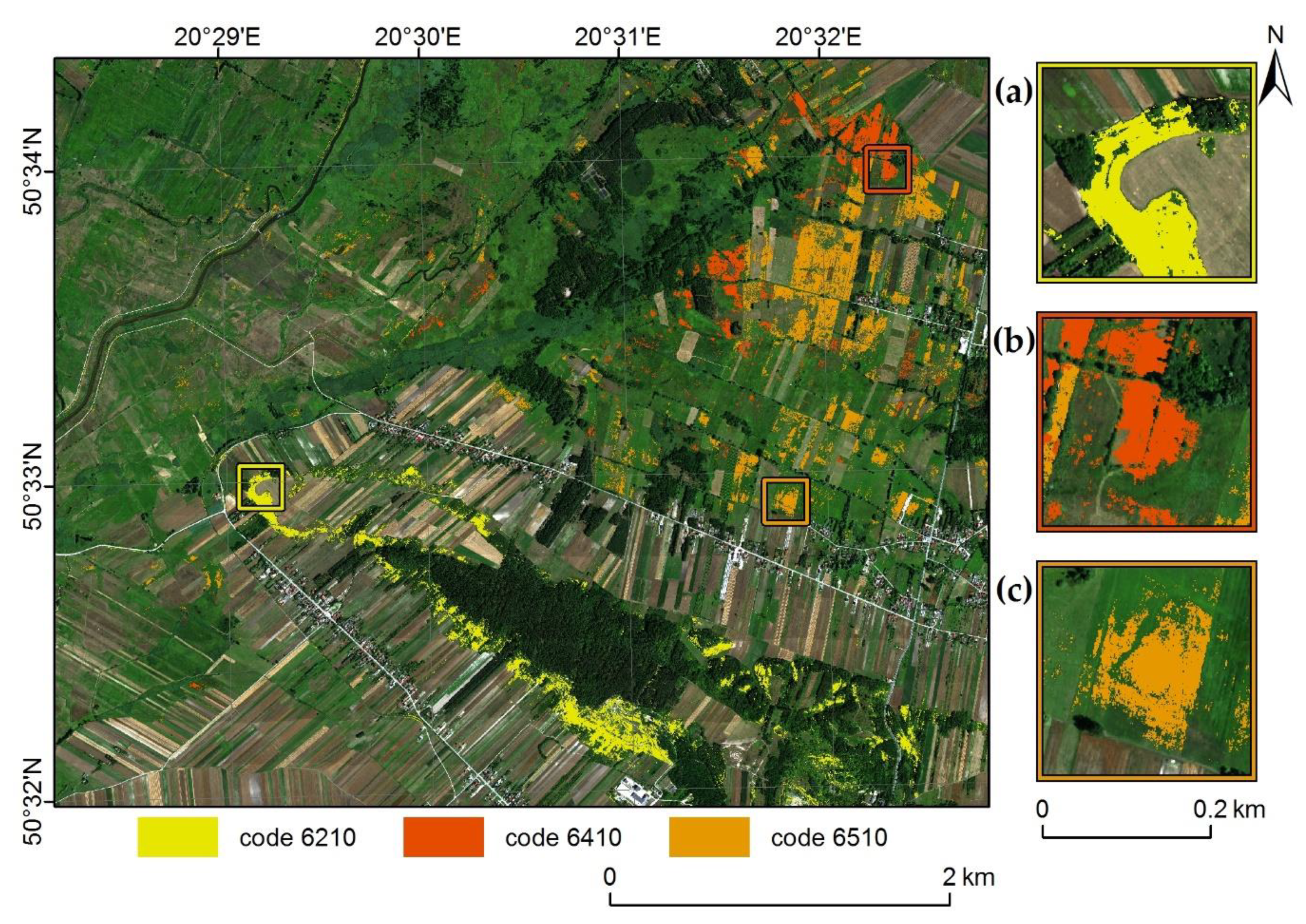
• Summer and early autumn were indicated as the optimal times to obtain remote sensing data to map grassland Natura 2000 habitats. Autumn is the best time of year to identify habitat 6510, while for habitats 6210 and 6410, results were slightly better for summer than autumn. Spring was the worst period of the year to identify non-forest Natura 2000 habitats.
• The use of fused multitemporal hyperspectral data allowed higher classification accuracy to be achieved than the use of data from a single collection. The fusion of hyperspectral data obtained from spring, summer, and autumn always provided the best results, regardless of habitat type. However, the fusion of data from summer and autumn provided comparable results to the fusion of data from all terms, and from a practical point of view it could be used instead. The difference in F1 accuracy between the classification results achieved by the merger of two (summer and autumn) versus three terms, regardless of the Natura 2000 habitat, is no more than 2%.
• For semi-natural dry grasslands and scrubland facies on calcareous substrates (code 6210), whose presence is most strongly associated with appropriate terrain conditions, the classification of hyperspectral data fused with topographic indices was much more effective than the classification of single date hyperspectral data, and comparable to data fusion performed with all available data.
• For Molinia meadows (code 6410), the best classification accuracy was obtained using a fusion of three-term multitemporal hyperspectral data and topographic indices; however, multitemporal fusion of only hyperspectral data from three terms can be assessed as comparably suitable.
• For lowland hay meadows (code 6510), whose presence is not related to particular topographical conditions, it was confirmed that fusion of hyperspectral data and topographic indices did not influence classification results, both single-date and multitemporal. The highest accuracy was obtained using fused multitemporal hyperspectral data from all terms; however, fused summer and autumn data provided also satisfactory results.

References

1. Turner, B.; Ii, B.T. Land Change Science. Int. Encycl. Hum. Geogr. 2009, 107–111. [Google Scholar] [CrossRef]
2. European Comission Council. Directive 92/43/EEC of 21 May 1992 on the conservation of natural habitats and of wild fauna and flora (OJ L 206 22.07.1992 p. 7). Doc. Eur. Community Environ. Law 2010, 568–583. [Google Scholar] [CrossRef]
3. Dimopoulous, P.; Chytry, M.; Loidi Arregui, J.J.; Etlicher, B.; Mazagol, P.-O.; Sacca, C.; Just, A.; Debarros, G.; Millet, J.; Savia, L.; et al. The survey of mapping projects in European countries: A focus on mapping methodology. Terr. Habitat Mapp. Eur. Overv. 2014, 55–72. [Google Scholar] [CrossRef]
4. Zlinszky, A.; Schroiff, A.; Kania, A.; Deák, B.; Mücke, W.; Vári, Á.; Székely, B.; Pfeifer, N. Categorizing grassland vegetation with full-waveform airborne laser scanning: A feasibility study for detecting natura 2000 habitat types. Remote Sens. 2014, 6, 8056–8087. [Google Scholar] [CrossRef]
5. Marcinkowska-Ochtyra, A.; Zagajewski, B.; Raczko, E.; Ochtyra, A.; Jarocińska, A. Classification of High-Mountain Vegetation Communities within a Diverse Giant Mountains Ecosystem Using Airborne APEX Hyperspectral Imagery. Remote Sens. 2018, 10, 570. [Google Scholar] [CrossRef]
6. Wald, L. Some terms of reference in data fusion. IEEE Trans. Geosci. Remote Sens. 1999, 37, 1190–1193. [Google Scholar] [CrossRef] [Green Version]
7. Serpico, S.; Bruzzone, L. A new search algorithm for feature selection in hyperspectral remote sensing images. IEEE Trans. Geosci. Remote Sens. 2001, 39, 1360–1367. [Google Scholar] [CrossRef]
8. Mücher, C.A.; Kooistra, L.; Vermeulen, M.; Haest, B.; Spanhove, T.; Delalieux, S.; Vanden Borre, J.; Schmidt, A.M. Object identification and characterization with hyperspectral imagery to identify structure and function of Natura 2000 habitats. In Proceedings of the GEOBIA 2010—The Geographic Object-Based Image Analysis Conference, Ghent, Belgium, 29 June–2 July 2010; Volume XXXVIII-4/C7, pp. 1–6. [Google Scholar]
9. Onojeghuo, A.O.; Onojeghuo, A.R. Object-based habitat mapping using very high spatial resolution multispectral and hyperspectral imagery with LiDAR data. Int. J. Appl. Earth Obs. Geoinf. 2017, 59, 79–91. [Google Scholar] [CrossRef]
10. Delalieux, S.; Somers, B.; Haest, B.; Spanhove, T.; Vanden Borre, J.; Mücher, C.A. Heathland conservation status mapping through integration of hyperspectral mixture analysis and decision tree classifiers. Remote Sens. Environ. 2012, 126, 222–231. [Google Scholar] [CrossRef]
11. Hufkens, K.; Thoonen, G.; Borre, J.V.; Scheunders, P.; Ceulemans, R. Habitat reporting of a heathland site: Classification probabilities as additional information, a case study. Ecol. Inform. 2010, 5, 248–255. [Google Scholar] [CrossRef]
12. Burai, P.; Deák, B.; Valkó, O.; Tomor, T. Classification of Herbaceous Vegetation Using Airborne Hyperspectral Imagery. Remote Sens. 2015, 7, 2046–2066. [Google Scholar] [CrossRef] [Green Version]
13. Marcinkowska-Ochtyra, A.; Zagajewski, B.; Ochtyra, A.; Jarocińska, A.; Wojtuń, B.; Rogass, C.; Mielke, C.; Lavender, S. Subalpine and alpine vegetation classification based on hyperspectral APEX and simulated EnMAP images. Int. J. Remote Sens. 2017, 38, 1839–1864. [Google Scholar] [CrossRef] [Green Version]
14. Jędrych, M.; Zagajewski, B.; Marcinkowska-Ochtyra, A. Application of Sentinel-2 and EnMAP new satellite data to the mapping of alpine vegetation of the Karkonosze Mountains. Pol. Cartogr. Rev. 2017, 49, 107–119. [Google Scholar] [CrossRef] [Green Version]
15. Kupková, L.; Červená, L.; Suchá, R.; Jakešová, L.; Zagajewski, B.; Březina, S.; Albrechtová, J. Classification of tundra vegetation in the Krkonoše Mts. National park using APEX, AISA dual and sentinel-2A data. Eur. J. Remote Sens. 2017, 50, 29–46. [Google Scholar] [CrossRef]
16. Feilhauer, H.; Dahlke, C.; Doktor, D.; Lausch, A.; Schmidtlein, S.; Schulz, G.; Stenzel, S. Mapping the local variability of Natura 2000 habitats with remote sensing. Appl. Veg. Sci. 2014, 17, 765–779. [Google Scholar] [CrossRef]
17. Sławik, Ł.; Niedzielko, J.; Kania, A.; Piórkowski, H.; Kopeć, D. Multiple Flights or Single Flight Instrument Fusion of Hyperspectral and ALS Data? A Comparison of their Performance for Vegetation Mapping. Remote Sens. 2019, 11, 970. [Google Scholar] [CrossRef]
18. Landmann, T.; Piiroinen, R.; Makori, D.M.; Abdel-Rahman, E.M.; Makau, S.; Pellikka, P.; Raina, S.K. Application of hyperspectral remote sensing for flower mapping in African savannas. Remote Sens. Environ. 2015, 166, 50–60. [Google Scholar] [CrossRef]
19. Camps-Valls, G.; Calpe-Maravilla, J.; Olivas, E.S.; Alonso-Chorda, L.; Gómez-Chova, L.; Martín-Guerrero, J.D.; Moreno, J. Robust support vector method for hyperspectral data classification and knowledge discovery. IEEE Trans. Geosci. Remote Sens. 2004, 42, 1530–1542. [Google Scholar] [CrossRef]
20. Raczko, E.; Zagajewski, B. Comparison of support vector machine, random forest and neural network classifiers for tree species classification on airborne hyperspectral APEX images. Eur. J. Remote Sens. 2017, 50, 144–154. [Google Scholar] [CrossRef] [Green Version]
21. Zhang, C.; Xie, Z. Object-based Vegetation Mapping in the Kissimmee River Watershed Using HyMap Data and Machine Learning Techniques. Wetlands 2013, 33, 233–244. [Google Scholar] [CrossRef]
22. Chan, J.C.-W.; Beckers, P.; Spanhove, T.; Borre, J.V. An evaluation of ensemble classifiers for mapping Natura 2000 heathland in Belgium using spaceborne angular hyperspectral (CHRIS/Proba) imagery. Int. J. Appl. Earth Obs. Geoinf. 2012, 18, 13–22. [Google Scholar] [CrossRef]
23. Corbane, C.; Alleaume, S.; Deshayes, M. Mapping natural habitats using remote sensing and sparse partial least square discriminant analysis. Int. J. Remote Sens. 2013, 34, 7625–7647. [Google Scholar] [CrossRef] [Green Version]
24. Stenzel, S.; Feilhauer, H.; Mack, B.; Metz, A.; Schmidtlein, S. Remote sensing of scattered Natura 2000 habitats using a one-class classifier. Int. J. Appl. Earth Obs. Geoinf. 2014, 33, 211–217. [Google Scholar] [CrossRef]
25. Marcinkowska, A.; Zagajewski, B.; Ochtyra, A.; Jarocińska, A.; Raczko, E.; Kupková, L.; Stych, P.; Meuleman, K. Mapping vegetation communities of the Karkonosze National Park using APEX hyperspectral data and Support Vector Machines. Misc. Geogr. 2014, 18, 23–29. [Google Scholar] [CrossRef] [Green Version]
26. Kopeć, D.; Michalska-Hejduk, D.; Sławik, Ł.; Berezowski, T.; Borowski, M.; Rosadziński, S.; Chormański, J. Application of multisensoral remote sensing data in the mapping of alkaline fens Natura 2000 habitat. Ecol. Indic. 2016, 70, 196–208. [Google Scholar] [CrossRef]
27. Zhang, C. Combining Hyperspectral and Lidar Data for Vegetation Mapping in the Florida Everglades. Photogramm. Eng. Remote Sens. 2014, 80, 733–743. [Google Scholar] [CrossRef] [Green Version]
28. Zagajewski, B.; Tømmervik, H.; Bjerke, J.W.; Raczko, E.; Bochenek, Z.; Kłos, A.; Jarocińska, A.; Lavender, S.; Ziółkowski, D. Intraspecific Differences in Spectral Reflectance Curves as Indicators of Reduced Vitality in High-Arctic Plants. Remote Sens. 2017, 9, 1289. [Google Scholar] [CrossRef]
29. Buck, O.; Millán, V.E.G.; Klink, A.; Pakzad, K. Using information layers for mapping grassland habitat distribution at local to regional scales. Int. J. Appl. Earth Obs. Geoinf. 2015, 37, 83–89. [Google Scholar] [CrossRef]
30. Marcinkowska-Ochtyra, A.; Jarocińska, A.; Bzdęga, K.; Tokarska-Guzik, B. Classification of Expansive Grassland Species in Different Growth Stages Based on Hyperspectral and LiDAR Data. Remote Sens. 2018, 10, 2019. [Google Scholar] [CrossRef]
31. Alcantara, C.; Kuemmerle, T.; Prishchepov, A.V.; Radeloff, V.C. Mapping abandoned agriculture with multi-temporal MODIS satellite data. Remote Sens. Environ. 2012, 124, 334–347. [Google Scholar] [CrossRef]
32. Prishchepov, A.V.; Radeloff, V.C.; Dubinin, M.; Alcantara, C. The effect of Landsat ETM/ETM+ image acquisition dates on the detection of agricultural land abandonment in Eastern Europe. Remote Sens. Environ. 2012, 126, 195–209. [Google Scholar] [CrossRef]
33. Rapinel, S.; Mony, C.; Lecoq, L.; Clément, B.; Thomas, A.; Hubert-Moy, L. Evaluation of Sentinel-2 time-series for mapping floodplain grassland plant communities. Remote Sens. Environ. 2019, 223, 115–129. [Google Scholar] [CrossRef]
34. Schuster, C.; Schmidt, T.; Conrad, C.; Kleinschmit, B.; Forster, M. Grassland habitat mapping by intra-annual time series analysis—Comparison of RapidEye and TerraSAR-X satellite data. Int. J. Appl. Earth Obs. Geoinf. 2015, 34, 25–34. [Google Scholar] [CrossRef]
35. Lawrence, R.L.; Wood, S.D.; Sheley, R.L. Mapping invasive plants using hyperspectral imagery and Breiman Cutler classifications (randomForest). Remote Sens. Environ. 2006, 100, 356–362. [Google Scholar] [CrossRef]
36. Govender, M.; Chetty, K.; Bulcock, H. A review of hyperspectral remote sensing and its application in vegetation and water resource studies. Water SA 2007, 33. [Google Scholar] [CrossRef]
37. Pohl, C.; Van Genderen, J.L. Review article Multisensor image fusion in remote sensing: Concepts, methods and applications. Int. J. Remote Sens. 1998, 19, 823–854. [Google Scholar] [CrossRef] [Green Version]
38. Kycko, M.; Zagajewski, B.; Lavender, S.; Romanowska, E.; Zwijacz-Kozica, M. The Impact of Tourist Traffic on the Condition and Cell Structures of Alpine Swards. Remote Sens. 2018, 10, 220. [Google Scholar] [CrossRef]
39. Ghamisi, P.; Rasti, B.; Yokoya, N.; Wang, Q.; Hofle, B.; Bruzzone, L.; Bovolo, F.; Chi, M.; Anders, K.; Gloaguen, R.; et al. Multisource and Multitemporal Data Fusion in Remote Sensing: A Comprehensive Review of the State of the Art. IEEE Geosci. Remote Sens. Mag. 2019, 7, 6–39. [Google Scholar] [CrossRef] [Green Version]
40. Yeadon, M.; King, M. A method for synchronising digitised video data. J. Biomech. 1999, 32, 983–986. [Google Scholar] [CrossRef]
41. Ka̧cki, Z.; Michalska-Hejduk, D. Assessment of biodiversity in Molinia meadows in Kampinoski National Park based on biocenotic indicators. Pol. J. Environ. Stud. 2010, 19, 351–362. [Google Scholar]
42. Nimbalkar, P.; Jarocinska, A.; Zagajewski, B. Optimal Band Configuration for the Roof Surface Characterization Using Hyperspectral and LiDAR Imaging. J. Spectrosc. 2018, 2018, 1–15. [Google Scholar] [CrossRef]
43. Sabat-Tomala, A.; Jarocińska, A.M.; Zagajewski, B.; Magnuszewski, A.S.; Sławik, Ł.M.; Ochtyra, A.; Raczko, E.; Lechnio, J.R. Application of HySpex hyperspectral images for verification of a two-dimensional hydrodynamic model. Eur. J. Remote Sens. 2018, 51, 637–649. [Google Scholar] [CrossRef] [Green Version]
44. Schläpfer, D.; Richter, R. Geo-atmospheric processing of airborne imaging spectrometry data. Part 1: Parametric orthorectification. Int. J. Remote Sens. 2002, 23, 2609–2630. [Google Scholar] [CrossRef]
45. Richter, R.; Schläpfer, D. ATCOR-4 User Guide; German Aerospace Center: Cologne, Germany, 2016. [Google Scholar]
46. Green, A.; Berman, M.; Switzer, P.; Craig, M. A transformation for ordering multispectral data in terms of image quality with implications for noise removal. IEEE Trans. Geosci. Remote Sens. 1988, 26, 65–74. [Google Scholar] [CrossRef] [Green Version]
47. Conrad, O.; Bechtel, B.; Bock, M.; Dietrich, H.; Fischer, E.; Gerlitz, L.; Wehberg, J.; Wichmann, V.; Böhner, J. System for Automated Geoscientific Analyses (SAGA) v. 2.1.4. Geosci. Model Dev. 2015, 8, 1991–2007. [Google Scholar] [CrossRef] [Green Version]
48. Dowling, T.I.; Gallant, J.C. A multiresolution index of valley bottom flatness for mapping depositional areas. Water Resour. Res. 2003, 39. [Google Scholar] [CrossRef]
49. Guisan, A.; Weiss, S.B. GLM versus CCA spatial modeling of plant species distribution. Plant Ecol. 1999, 143, 107–122. [Google Scholar] [CrossRef]
50. Weiss, A. Topographic position and landforms analysis. Poster Present. ESRI User Conf. San Diego, CA (2001). Available online: http://www.jennessent.com/downloads/TPI-poster-TNC_18x22.pdf (accessed on 28 September 2019).
51. Beven, K.J.; Kirkby, M.J. A physically based, variable contributing area model of basin hydrology. Hydrol. Sci. Bull. 1979, 24, 43–69. [Google Scholar] [CrossRef]
52. Moore, I.D.; Grayson, R.B.; Ladson, A.R. Digital terrain modelling: A review of hydrological, geomorphological, and biological applications. Hydrol. Process. 1991, 5, 3–30. [Google Scholar] [CrossRef]
53. Shaw, R.L.; Booth, A.; Sutton, A.J.; Miller, T.; Smith, J.A.; Young, B.; Jones, D.R.; Dixon-Woods, M. Finding qualitative research: An evaluation of search strategies. BMC Med. Res. Methodol. 2004, 4, 5. [Google Scholar] [CrossRef]
54. Böhner, J.; Köthe, R.; Conrad, O.; Gross, J.; Ringeler, A.; Selige, T. Soil regionalisation by means of terrain analysis and process parameterisation. Eur. Soil Bur. 2001, 7, 213–222. [Google Scholar]
55. Liaw, A.; Wiener, M. Classification and Regression by randomForest. R News 2002, 2–3, 18–22. [Google Scholar]
56. R Core Team. R: A Language and Environment for Statistical Computing; R Foundation for Statistical Computing: Vienna, Austria, 2018. [Google Scholar]
57. Breiman, L. Random forests. Mach. Learn. 2001, 45, 5–32. [Google Scholar] [CrossRef]
58. Breiman, L. Prediction Games and Arcing Algorithms. Neural Comput. 1999, 11, 1493–1517. [Google Scholar] [CrossRef] [PubMed]
59. Cutler, D.R.; Edwards, T.C.; Beard, K.H.; Cutler, A.; Hess, K.T.; Gibson, J.; Lawler, J.J. Random forests for classification in ecology. Ecology 2007, 88, 2783–2792. [Google Scholar] [CrossRef]
60. Kim, J.-H. Estimating classification error rate: Repeated cross-validation, repeated hold-out and bootstrap. Comput. Stat. Data Anal. 2009, 53, 3735–3745. [Google Scholar] [CrossRef]
61. Ghosh, A.; Fassnacht, F.E.; Joshi, P.; Koch, B. A framework for mapping tree species combining hyperspectral and LiDAR data: Role of selected classifiers and sensor across three spatial scales. Int. J. Appl. Earth Obs. Geoinf. 2014, 26, 49–63. [Google Scholar] [CrossRef]
62. Champagne, C.; McNairn, H.; Daneshfar, B.; Shang, J. A bootstrap method for assessing classification accuracy and confidence for agricultural land use mapping in Canada. Int. J. Appl. Earth Obs. Geoinf. 2014, 29, 44–52. [Google Scholar] [CrossRef] [Green Version]
63. Stehman, S.V.; Czaplewski, R.L. Design and analysis for thematic map accuracy assessment: Fundamental principles. Remote Sens. Environ. 1998. [Google Scholar] [CrossRef]
64. Congalton, R.G. A review of assessing the accuracy of classifications of remotely sensed data. Remote Sens. Environ. 1991, 37, 35–46. [Google Scholar] [CrossRef]
65. Van Rijsbergen, C.J. Information Retrieval, 2nd ed.; Butterworths: London, UK, 1979. [Google Scholar]
66. Potvin, C.; Roff, D.A. Distribution-Free and Robust Statistical Methods: Viable Alternatives to Parametric Statistics. Ecology 1993, 74, 1617–1628. [Google Scholar] [CrossRef]
67. Maślanka, M. Factors influencing ground point density from Airborne Laser Scanning—A case study with ISOK Project data. Ann. Geomat. 2016, 14, 511–519. [Google Scholar]
68. Szostak, M.; Wężyk, P.; Pająk, M.; Haryło, P.; Lisańczuk, M. Determination of the spatial structure of vegetation on the repository of the mine “Fryderyk” in Tarnowskie Góry, based on airborne laser scanning from the ISOK project and digital orthophotomaps. Geodesy Cartogr. 2015, 64, 87–99. [Google Scholar] [CrossRef]
69. Raab, C.; Stroh, H.G.; Tonn, B.; Meißner, M.; Rohwer, N.; Balkenhol, N.; Isselstein, J. Mapping semi-natural grassland communities using multi-temporal RapidEye remote sensing data. Int. J. Remote Sens. 2018, 39, 5638–5659. [Google Scholar] [CrossRef]
70. Haest, B.; Borre, J.V.; Spanhove, T.; Thoonen, G.; Delalieux, S.; Kooistra, L.; Mücher, C.A.; Paelinckx, D.; Scheunders, P.; Kempeneers, P. Habitat Mapping and Quality Assessment of NATURA 2000 Heathland Using Airborne Imaging Spectroscopy. Remote Sens. 2017, 9, 266. [Google Scholar] [CrossRef]
71. Woodcock, C.E.; Strahler, A.H. The factor of scale in remote sensing. Remote Sens. Environ. 1987, 21, 311–332. [Google Scholar] [CrossRef]
72. Mack, B.; Roscher, R.; Stenzel, S.; Feilhauer, H.; Schmidtlein, S.; Waske, B. Mapping raised bogs with an iterative one-class classification approach. ISPRS J. Photogramm. Remote Sens. 2016, 120, 53–64. [Google Scholar] [CrossRef]
73. Kopeć, D.; Zakrzewska, A.; Halladin-Dąbrowska, A.; Wylazłowska, J.; Kania, A.; Niedzielko, J. Using Airborne Hyperspectral Imaging Spectroscopy to Accurately Monitor Invasive and Expansive Herb Plants: Limitations and Requirements of the Method. Sensors 2019, 19, 2871. [Google Scholar] [CrossRef]
Figure 1. Study area location. Ostoja Nidziańska (a), basemap: HySpex image in natural colour Red, Green, Blue (RGB) composition, acquired in September 2017; Central Europe (b), basemap: © EuroGeographics for the administrative boundaries.
Remotesensing 11 02264 g001
Figure 2. Selected Natura 2000 habitats in Ostoja Nidziańska area: (a) 6210; (b) 6410; (c) 6510 (photos by: B. Tokarska-Guzik, B. Babczyńska-Sendek and T. Nowak, all taken in July).
Remotesensing 11 02264 g002
Figure 3. Overall accuracies for each dataset in three campaigns (C1, C2, C3—campaign number, MNF—minimum noise fraction, TOPO—topographic indices).
Remotesensing 11 02264 g003
Figure 4. F1 classification accuracies for all datasets in three campaigns calculated for habitat: code 6210 (a); code 6410 (b) and code 6510 (c) (C1, C2, C3—campaign number, MNF—minimum noise fraction, TOPO—topographic indices).
Remotesensing 11 02264 g004
Figure 5. Distribution of all classified habitats based on the classification with the highest average F1 = 78.9% (C1_C2_C3_MNF + TOPO) (codes: 6210 (a); code 6410 (b) and code 6510 (c); basemap: HySpex image in natural red, green, blue (RGB) composition, acquired in July 2017).
Remotesensing 11 02264 g005