Retrieval of Suspended Particulate Matter in Inland Waters with Widely Differing Optical Properties Using a Semi-Analytical Scheme

Abstract

Suspended particulate matter (SPM) directly affects the underwater light field and, as a consequence, changes the water clarity and can reduce the primary production. Remote sensing-based bio-optical modeling can provide efficient monitoring of the spatiotemporal dynamics of SPM in inland waters. In this paper, we present a novel and robust bio-optical model to retrieve SPM concentrations for inland waters with widely differing optical properties (the Tietê River Cascade System (TRCS) in Brazil). In this system, high levels of Chl-a concentration of up to 700 mg/m³, turbidity up to 80 NTU and high CDOM absorption highly complicate the optical characteristics of the surface water, imposing an additional challenge in retrieving SPM concentration. Since K_d is not susceptible to the saturation issue encountered when using remote sensing reflectance (R_rs), we estimate SPM concentrations via K_d. K_d was derived analytically from inherent optical properties (IOPs) retrieved through a re-parameterized quasi-analytical algorithm (QAA) that yields relevant accuracy. Our model improved the estimates of the IOPs by up to 30% when compared to other existing QAAs. Our developed bio-optical model using K_d(655) was capable of describing 74% of SPM variations in the TRCS, with average error consistently lower than 30%.

1. Introduction

Suspended particulate matter (SPM—see

Table 1. List of acronyms and symbols.

Acronym	Description
AOPs	Apparent optical properties
IOPs	Inherent optical properties
BB	Barra Bonita Hydroelectric Reservoir
BAR	Bariri Hydroelectric Reservoir
IBI	Ibitinga Hydroelectric Reservoir
NAV	Nova Avanhandava Hydroelectric Reservoir
CDOM	Colored dissolved organic matter
Chl-a	Chlorophyll-a
QAA	Quasi analytical algorithm
NAP	Non-algae particles
OSC	Optical significant compounds
TRCS	Tietê River Cascade System
Symbol	Parameter	Unit
γ	Geometrical light factor	-
Rrs	Remote sensing reflectance above water surface	sr−1
rrs	Remote sensing reflectance below water surface	sr−1
Υ	Spectral power of particle backscattering coefficient	-
S	Spectral slope for non-algae particles (Snap) or CDOM (Scdom)	nm−1
SPM	Suspended particulate matter	mg.L−1
Ed(λ)	Spectral downwelling irradiance below the water surface	W.m−2. nm−1
Es(λ)	Spectral downwelling irradiance incident onto the water surface	W.m−2. nm−1
Lt(λ)	Spectral total radiance above water surface	W.m−2.sr−1.nm−1
Lsky(λ)	Spectral incident sky radiance	W.m−2.sr−1.nm−1
Kd(λ)	Downwelling diffuse attenuation coefficient	m−1
a(λ), at(λ)	Spectral total absorption coefficient (a(λ) = acdom(λ)+ ap(λ)+ aw(λ))	m−1
acdom(λ)	Spectral absorption coefficient of CDOM	m−1
ap(λ)	Spectral absorption coefficient of particulate matter (ap(λ) = ap(λ)+ anap(λ))	m−1
aφ(λ)	Spectral absorption coefficient of phytoplankton pigments	m−1
anap(λ)	Spectral absorption coefficient of non-algae particles	m−1
aw(λ)	Spectral absorption coefficient of water	m−1
atnw(λ), at-w	Spectral non-water total absorption coefficient	m−1
b(λ)	Spectral scattering coefficient	m−1
bb(λ)	Spectral total backscattering coefficient (bb(λ)=bbp(λ)+ bbw(λ))	m−1
bbp(λ)	Spectral total backscattering coefficient of particulate matter	m−1
bbw(λ)	Spectral total backscattering coefficient of water	m−1
u(λ)	Ratio of backscattering coefficient to the sum of absorption and backscattering coefficient (bb(λ)/bb(λ)+ a(λ))	-
Z	Depth within the water column	m
zi	Depth for time - i	m
ZSD	Secchi disk depth	m
Q	Ratio between
T	radiance transmittance
t	time of scan	ms
$\gamma$	water to air internal reflection coefficient
${\lambda }_0$	Reference wavelength	nm

for symbols and acronyms) is a major component of the aquatic environment, composed by organic and inorganic fractions. It plays an important role in the hydrophysical functioning and biogeochemical cycles of inland waters [1]. It essentially controls, through the absorption and backscattering of light and the turbidity and transparency of the water column, which can affect the total available energy for photosynthetic activities [2]. Furthermore, SPM controls the transport of materials and contaminants in aquatic systems, representing an index of general uses of water resources [3]. Thus, mapping the distribution of SPM concentration is considered critical in water resource management. High levels of SPM may alter the nutrient composition available in water and decreases the water clarity, affecting the light penetration through the water column [4]. The gradient of available energy underwater largely determines the biogeochemical cycles and biodiversity of aquatic organisms [5,6,7].

Although the SPM in inland water systems has been monitored using several different approaches [8], remote sensing can be considered the most promising and efficient way to map the large-scale spatiotemporal dynamics of SPM [9,10]. Traditionally, SPM could be estimated from inherent (IOPs) or apparent (AOPs) optical properties using empirical or analytical models [11]. Using the IOPs, SPM concentrations can be obtained by employing a spectral absorption index (SAI [12]) or by applying empirical regressions with backscattering coefficient (b_b) [13]. Using the AOPs, SPM can be derived from the remote sensing reflectance (R_rs) from unique or band ratios [14,15]. Establishing a reliable model to estimate SPM concentration using R_rs in inland waters, however still remains a challenge, because R_rs saturates at certain levels of SPM [16]. Further, the chlorophyll-a (Chl-a), colored dissolved organic matter (CDOM), and organic and inorganic fractions of SPM respond differently to the incident energy, resulting in a wide range of magnitudes and shapes of R_rs spectra [17,18]. The Tietê River is a representative case that presents widely ranging IOPs, where the phytoplankton absorption coefficient (a_∅) at 443 nm ranges from 0.02 to 10.9 m⁻¹ [19].

The Tietê River is the longest river in São Paulo State, running more than 1000 km before meeting the Parana River, which later becomes the Plata River reaching the Atlantic Ocean. The Tiete River is an important water resource for the communities at the local scale, providing valuable drinking water, food sources, irrigation, water for industrial use, transportation and recreation [20]; thus, the water quality of the river is considered a critical issue in this region. A series of six hydroelectrical reservoirs along the Tietê River are constantly filtering the water, and intensive anthropogenic activities occur within the catchments (e.g., agriculture, dredging, industrial production and fishing activities). Therefore, different types of water draining the surrounding catchments are impacting directly the dynamics of the SPM in the Tiete River [21,22], resulting in a wide range of magnitude concentration and varying composition of the SPM. Several attempts were made to assess the spatiotemporal patterns of the SPM in the Tietê River Cascade System (TRCS); however, they were not successful in retrieving a robust result. For instance, empirical algorithms have been used to estimate the SPM over a specific [23] or combined reservoirs [18]. However a universal model that accounts for both a large variability (and spatially heterogeneous) in SPM concentrations and its varying biogeochemical composition still does not exist by considering K_d, retrieved from an semianalytical scheme, as the main predictor of SPM in wide ranges.

In this paper we used diffuse attenuation coefficient (K_d) as a key parameter for the SPM retrieval. K_d depends on several factors, such as depth (z), incident light (E_d), IOPs (a and b_b) and optically significant constituents (OSCs—Chl-a, CDOM and SPM). In the inland water systems such as the TRCS, SPM concentrations are the main OSC that control the K_d values [24]. As an AOP, K_d is largely determined by the IOPs (a and b_b) and secondarily on the light field geometry [25]. Therefore, K_d is considered more stable than the R_rs in estimating SPM, because it is directly derived by summing the IOPs [25], while R_rs is a function of the ratio of IOP, due to the analytical configuration of absorption and backscattering. In addition, K_d is also relatively easier to validate compared to SPM models based on b_b [26,27]. Thus, K_d can be used efficiently to map SPM dynamics over inland waters where the SPM concentration varies widely, which has only been used so far in some coastal waters [27].

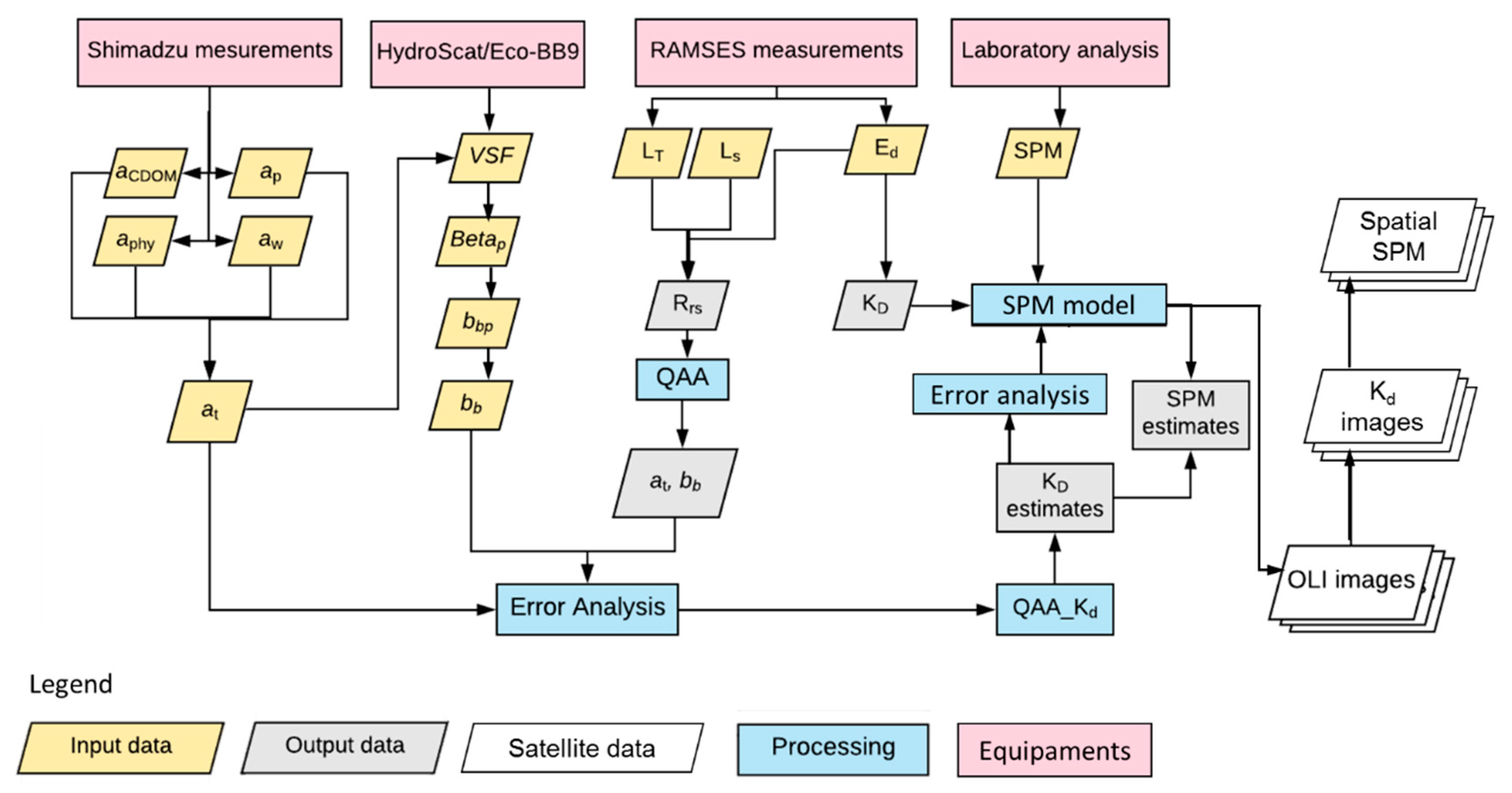
We aim to develop a semi-analytical scheme to estimate SPM in the TRCS that is sensitive enough to capture the widely varying effects of OSCs. For this, K_d is estimated based on the methods by Lee et al. [28], derived from the IOPs (a and b_b) estimated using a re-parameterized version of a quasi-analytical algorithm (QAA [29]). The QAA was tested for the TRCS [20,30] and the results suggested that further re-parameterizations of the QAA are required for more accurate results. The K_d model from Lee et al. (2013 [28], 2015 [31]) was also evaluated for other inland waters [22,30], which provided the lowest error when compared with other published algorithms to retrieved K_d. However, the suitability of Lee’s model was never tested for the entire TRCS where the optical composition of surface water varies over reservoirs. Therefore, the specific objectives of this paper are to (i) re-parameterize the QAA considering the optical composition and the available spectral bands onboard Landsat-8, (ii) compare our results with other versions of QAA tuned for inland waters, (iii) evaluate the suitability OLI bands to estimate Kd for the first time, and (iv) evaluate the influence of different water compositions on SPM estimates.

2. Materials and Methods

2.1. Fieldsite and Dataset

The TRCS is located in the southeast of Brazil and contains six reservoirs—Barra Bonita (BB, 22°31’S, 48°32’W), Bariri (BAR, 22° 9’S,48°44’W), Ibitinga (IBI, 21°45’S, 48°59’), Promissão (21°48’ S, 49°23’W), Nova Avanhandava (NAV, 21°71’S, 50°12’W) and Três Irmãos (21°38’S, 51°32’) (Figure 1). Among them, BB, BAR, IBI and NAV reservoirs produce more than 90% of hydroelectric energy from the entire cascade (resulting in 763 MW [30]). BAR, IBI and NAV are run-of-river reservoirs, whereas BB is an accumulation reservoir [32].

BB is a eutrophic environment [33]; BAR and IBI are considered meso-to-eutrophic environments [34], while NAV is considered as oligo-to-mesotrophic waters [18]. Eight field works were conducted in the TRCS, two per each reservoir (

Table 2. Study sites and sampled parameters in Barra Bonita, Bariri, Ibitinga and Nova Avanhandava reservoirs (see Table 1 for acronyms and symbols).

Reservoirs	Field Campaign ID	n	Time Acquisition	Radiometric Variables	Water Quality and Physical Parameters
Barra Bonita	BB1/BB2	20/20	May/October, 2014	Lt, Lsky Es, and Ed at (acdom, aphy, anap) and bb	Turbidity, ZSD, SPM, PIM, POM, Chl-a, Wind Speed and Depth.
Bariri	BAR1	30	August, 2016
	BAR2	18	June, 2017
Ibitinga	IBI1	30	July, 2016
	IBI2	16	June, 2017
Nova Avanhandava	NAV1/NAV2	20/20	May/September, 2014

). The sampling sites for radiometric, water quality and physical parameters measurements were defined according to Rodrigues et al. (2016) [35].

According to the land use and land cover (LULC) map in Figure 1, the upstream area is dominated by industrial and artificial areas, responsible for high levels of sewage discharges. In the downstream regions, agriculture and pasture are the main economic activities, which also can act as a pollution source due to irrigation and runoffs from herbicides and other poisons from bare soil and shrub lands.

Turbidity (NTU), wind speed (m/s), Secchi disk depth (Z_SD; m) and bottom depth (m) were triplicated, measured using a with a portable turbidimeter, anemometer, a Secchi disk (diameter of 30 cm), and a depth gauge, respectively. Since the ZSD is much lower than the average depth of the reservoir, all reservoirs were considered as optically deep waters, where the bottom effects are negligible. SPM concentrations and organic and inorganic fractions were retrieved using water samples (250 mL to 1 L, depending on the fieldwork aiming to avoid the filter’s saturation) were filtered through Whatman GF/F filters (47 mm diameter and 0.7 pore size). For the SPM, the filtrated matter retained in the filters was dried in the oven at 100 °C for 12 hours and weighed to establish the organic fraction. Then, they were put in the muffle furnace at 550 °C for 30 min before being weighed again to establish the inorganic fraction (American Public Health Association protocol [36]). For Chl-a, the concentrations were determined using the filtrate in filters obtained from filtration using a vacuum pressure pump in the darkness. Then, the Chl-a pigments were extracted using the acetone method. The extracted samples were submitted to the absorbance readings at 620 and 675 nm, which were used to compute the Chl-a concentrations, as described in Golterman et al. (1978) [37].

Radiometric measurements (E_d, E_s, L_sky and L_t) were obtained using TriOS hyperspectral radiometers (RAMSES TriOS ^®), over 400 to 900 nm wavelength. Measured radiance and irradiance (at 3.3 nm resolution) were interpolated to 1 nm resolution [38,39]. The R_rs variable was calculated using the spectral glint removal method [40], which is considered the most reliable [41]. We measured the particulate absorbance using a dual-beam UV-2600 UV–VIS spectrophotometer (SHIMADZU, Japan) at 1 nm resolution, over 280 to 800 nm. The transmittance-reflectance (T-R) method was used to calculate the particulate absorption (a_p = a_nap+ a_φ) described in Tassan and Ferrari (1995, 1998) [42,43]. To bleach the organic fraction of particulate, samples were washed using hypoclorite solution (NaClO at 10%). We used an absorption coefficient of cdom (a_cdom) established by Bricaud et al. (1995) [44], which uses a reference correction—a mean absorption value over 700 and 750 nm was subtracted from the entire spectrum curves.

Integration of volume scattering function (VSF) retrieved the backscattering coefficients from HydroScat-6P (HobiLabs, Bellevue-USA) and ECOBB-9 (WetLabs, Philomath-USA) measurements [20]. EcoBB-9 was used after the calibration process, whilst HydroScat-6P did not have such information. The absorption correction was made using laboratory measurements, and exponential fitting was applied to standardize the wavelengths to be in accordance with the outputs from the QAA. A flowchart showing the methodology described in this section is given in Figure 2.

2.2. K_d from IOPs

K_d were estimated using IOPs obtained from QAA modeling through the seven steps (Figure 3). Version 5 of the QAA (v5, [29]) has been empirically calibrated in coastal waters, where a_t(55x) might be less than 0.5 m⁻¹. Broader applications for inland water require several site-specific adaptations, mainly in the empirical steps [45,46,47]. The main error sources are related to (i) the reference wavelength (λ₀) and the estimations of absorption coefficient and (ii) the spectral power slope (Υ) used to compute b_b [48,49,50]. Furthermore, the empirical steps in the QAA also depend on the location of the sampled dataset [51]. The former limitation implies that re-parameterization of the coefficients is necessary because the optical conditions of water are distinct from the original study sites.

The QAA derives a and b_b from R_rs, which is referred to as Part I [54]. The second part of the QAA, which determines specific coefficients of each optically active component, was not assessed in this paper. The main changes in the parameters used in the QAA steps to improve its performance for inland waters were adapted from published results and are summarized in

Table 3. QAA steps and adaptations from Lee et al. (2002) [29], Zhu and Yu (2013) [51], Wang et al. (2017) [55], Ogashawara et al. (2016) [56], Watanabe et al. (2016) [20], Rodrigues et al. (2018) [18]. Steps 3, 5 and 6 were omitted because changes in the QAA were not made.

Step	Par.	1	2	3	4	5	6
0	$r_{rs}$	T = 0.52	T = 0.52	$=\frac{R_{rs}\left(\lambda \right)}{\alpha \left(\lambda \right)+\beta \left(\lambda \right)R_{rs}\left(\lambda \right)}$	-	-	-
		$\gamma Q$ = 1.7	$\gamma Q$ = 1.7
1	$u\left(\lambda \right)$	g0 = 0.089	-	-	-	-	-
		g1 = 0.125	-	-
2.1	$a_t\left({\lambda }_0\right)$	${\lambda }_0\ge 55x$	555	680	-	709	709
		h0 = −1.146	−1.226	−0.0852		−0.77	−1.148
		h1 = −1.366	−1.214	0.8650		0.099	2.814
		h2 = −0.469	−0.35	0.9398		0.056	−5.813
2.2	$\chi$	$\alpha =5$	-	-	-	-	0.05
		${\lambda }_1=443$	440	680 *	412	443	443
		${\lambda }_2=490$	490	490	560	665	665
		${\lambda }_3=667$	640	-	665	620	681
		${\lambda }_4=490$	490	-	443	443	443
4	${\rm Y}$	$y_0=$ 2.0	-	m = 1.75 *	-	1.0–1.9	–
		$y_1=$ 1.2		n = −0.05		1.3–1.5	–
		$y_2=$ −0.9		-		0.1–0.8	–
		${\lambda }_5=443$		-		${\lambda }_5=443$	665/754 **
6	$a\left(\lambda \right)$	C1= 1	-	-	rrs(${\lambda }_4$)/rrs(${\lambda }_0$)	-	-

* Band ratio = (680/490) and quadratic fit were used; ${\rm Y}$ = m × b_bp(680)ⁿ; ** band ratio to establish ${\rm Y}$ instead of 443/${\lambda }_0$.

.

We modified four steps of the original framework of the QAA to establish a QAA specific for the TRCS (QAA_TRCS). In the ‘zero’ step, we computed r_rs using spectral coefficients as described in [55] instead of using the fixed values of 0.52 and 1.7 (Lee et al., 2002 [29]), which provides better results for inland waters. The parameters in the empirical steps 2 and 3, in Figure 3, were not recalibrated. The λ₀ originally defined as 55x by Lee et al. (2002) were displaced towards 655 nm where the water absorption is the major contributor to a_t (Figure S1).

To compute χ, we modified the bands by replacing the 490 and 667 nm bands in the original QAA (Lee et al., 2002), with the bands at 561 and 482 nm, respectively. The use of 561 nm compensates the CDOM effects [56]. Another relevant change was to consider the multiplication factor in the denominator of χ, where we adapted the values of 5 for turbid environments (BB2 and BAR1) and 2 for non-turbid waters (<10 NTUs). The entire scheme can be found in Table S1.

The coefficients to retrieve a_t in (λ₀) can be recalibrated using in situ datasets in step 2 [20,30,51]. We used optimization processing to define the best band combination for computing the χ factor [20,30]. On the other hand, the Υ factor can be established for different purposes with other spectral bands [55] or by testing new coefficients [20]. Comparisons between the original version of the QAA (V5) and the newly defined steps of QAA_TRCS are shown in Table S1.

The outputs of the QAA, a and b_b, allow the K_d values to be computed as Equation (1):

$$K_{d\_QAA}\left(z,\lambda \right)=\left(1+m_0 \times {\theta }_s\right)a\left(\lambda \right)+(1-\gamma \frac{b_{bw}\left(\lambda \right)}{b_b\left(\lambda \right)})\times m_1\times \left(1-m_2\times e^{-m_3\times a\left(\lambda \right)}\right)b_b\left(\lambda \right),$$

(1)

where $K_{d\_QAA}\left(z,\lambda \right)$ is the K_d calculated from the QAA using OLI/Landsat-8 bands; $m_{0-3}$ and $\gamma$ are set to 0.005, 4.26, 0.52, 10.8, and 0.265, respectively, which are the coefficients obtained via Hydrolight simulations [28]. ${\theta }_s$ is the solar zenith angle (considered as 30°); $b_{bw}\left(\lambda \right)$ is the backscattering coefficient for water molecules (adopted from [53]); and a and b_b are the spectral coefficients derived through the QAA model [29].

2.3. K_d Reference

To establish the SPM model for the TRCS, we used in situ K_d as a predictor variable to calibrate the satellite images in the later steps. K_d values were retrieved from the field measurements of normalized irradiances, E_d and E_s, by using the irradiance sensors with the cosine collector of Ramses TriOS. Here, we refer the reference in situ K_d as K_{d_r} while the QAA driven K_d is referred to as K_{d_QAA}. K_d is mathematically described as an exponential function that represents the decrease of light, i.e., the reduction of available $E_d^{-}$ within the water column at a certain depth (z) [39] (Equation (2)).

$$K_d\left(z,\lambda \right)= -\frac{1}{E_d^{-}\left(\lambda \right)}\frac{d{E}_d^{-}}{dz}$$

(2)

The in situ measurements of E_d⁻, also called E_d(z_i), are affected by changes of sun geometry that result in variability of incident light field and consequently cause uncertainties in K_{d_r}. In order to minimize the illumination variability, we normalized to E_d(z) based on Mueller (2000) [38] and Mishra et al. (2005) [57] (Equation (3)):

$$E^{\prime }{}_d\left(z_i,\lambda \right)= -\frac{E_d\left(z_i,\lambda \right)E_s\left(t\left(z_1\right),\lambda \right)}{E_s\left(t\left(z_i\right),\lambda \right)}$$

(3)

The normalization factor is defined as the ratio between $E_s$ at the first sensor scan at t(z₁), $E_s\left(t\left(z_1\right),\lambda \right)$ and the following sensor scans along the depth at t(z_i) with t representing time of scans (ms), $E_s\left(t\left(z_i\right),\lambda \right)$. $E_s$ is the downwelling irradiance measured from the roof of the boat, and $E^{\prime }{}_d\left(z_i,\lambda \right)$ is the normalized E_d within water column in all downward directions [39]. Finally, the reference values of K_{d_r} were computed as Equation (4):

$$K_{d\_r}\left(z,\lambda \right)= -\frac{1}{E^{\prime }{}_d\left(\lambda \right)}\frac{d{E}^{\prime }{}_d}{dz}$$

(4)

2.4. SPM Modeling

SPM concentration was determined as the criterion variable, estimated based on the scores of K_{d_r}. The linear, quadratic, power and exponential fits were tested using K_{d_r} at 443, 482, 561 and 655 nm. The best fit, based on higher correlation coefficients (

Table 4. The best fits between K_{d_r} resampled for Operational Land Imager (OLI) bands (onboard Landsat-8) and SPM concentrations considering the entire TRCS’s dataset. a, b and c are the coefficients for linear (ax+b); quadratic (ax ²+bx+c); power (axb) and exponential (aln(x)+b) equations.

Model ID	OLI Band	a	b	c	r	Fit
M1	443	3.17	−2.57	-	0.73	Linear
M2	482	0.22	2.27	−0.53	0.79	quadratic
M3	561	3.50	1.39	-	0.61	power
M4	655	2.51	1.64	-	0.74	power

) was chosen, which is the model using K_{d_r}(482) that yielded r = 0.79, followed by K_{d_r}(655) with r = 0.74. The 655 nm band is also considered suitable for turbid inland waters [57,58,59].

QAA_TRCS equations were applied to the atmospherically corrected OLI images (

Table 5. OLI/Landsat-8 images used for mapping SPM concentrations.

Coverage Area	Path/Row	Overpass Date	Overpass Time (UTC)	Gap *
BB2	220/076	10/13/2014	13:10:45	3h10m
BAR1	220/076	08/15/2016	13:10:36	2h05m
IBI1	221/075	07/21/2016	13:16:18	3h00m
NAV1	222/075	05/02/2014	13:22:42	2 days

* Considering the samples taken nearest the images acquisition.

) level 2 product, i.e., Landsat 8 Surface Reflectance Code (LASRC) [60]. LASRC provides surface reflectance at suitable spatiotemporal resolutions for monitoring the dynamics of inland waters [61]. Previous works have shown that different water quality parameters, such as chlorophyll-a and turbidity, are well estimated via OLI images [62]. To retrieve R_rs images, the LASRC products were divided by 3.1415, and then, the scale factor was applied (0.0001 [60]). Finally, the QAA processing scheme (Table S1) and images of a_t and b_b were generated. Images covering the remaining reservoirs (BB1, IBI1, NAV2) were not used for the analysis due to heavy cloud cover.

The IOPs images were used as input of Equation (1) and retrieved an image of K_{d_QAA}. Sequentially, M2 and M4 (Table 4) were applied to the K_{d_QAA} images to map the SPM concentration in each reservoir. The modeled results were validated by comparing with the in situ SPM concentrations and SPM derived from images via K_d.

2.5. Accuracy Assessment

The a_t and b_b derived by QAAs (Table 4 and Table S1) were compared with the a_t and b_b obtained in laboratory and in situ, respectively. To assess the accuracy, we used the root mean squared error (RMSE in sr ⁻¹); normalized root mean squared error (nRMSE in %); bias (δ in sr ⁻¹); mean absolute percentage error (MAPE in %); and Pearson correlation coefficient (Equations (5)–(9), respectively).

$$RMSE= \sqrt{\frac{1}{n}{\displaystyle \sum }_{i=1}^n{\left(x_{e,i}-x_{m,i}\right)}^2}$$

(5)

$$nRMSE= \frac{RMSE}{\left(\max (x_{m,i}\right)- \min \left(x_{m,i}\right))}\times 100$$

(6)

$$\delta = \frac{1}{n}{\displaystyle \sum }_{i=1}^n\left(x_{e,i}-x_{m,i}\right)$$

(7)

$$MAPE=\frac{1}{n} {\displaystyle \sum }_{i=1}^n\frac{\left|x_{e,i}-x_{m,i}\right|}{x_{m,i}}\times 100$$

(8)

$$r={\displaystyle \sum }_{i=1}^N\left[\frac{x_{m,i}-\left(\frac{1}{N}{{\displaystyle \sum }}_{j=1}^N{x}_{e,j}\right)}{{\left(\frac{1}{N-1}{{\displaystyle \sum }}_{k=1}^N{\left[x_{m,k}-\left(\frac{1}{N}{{\displaystyle \sum }}_{l=1}^N{x}_{m,l}\right)\right]}^2\right)}^{0.5}}\right]\left[\frac{x_{e,i}-\left(\frac{1}{N}{{\displaystyle \sum }}_{j=1}^N{x}_{e,j}\right)}{{\left(\frac{1}{N-1}{{\displaystyle \sum }}_{k=1}^N{\left[x_{e,k}-\left(\frac{1}{N}{{\displaystyle \sum }}_{l=1}^N{x}_{e,l}\right)\right]}^2\right)}^{0.5}}\right]$$

(9)

where $x_{e,i}$ is the estimated values, $x_{m,i}$ is the measurements, min and max correspond to the minimum and maximum values of the dataset, and n is the number of samples. K_d derived from the QAA were assessed by comparing with K_{d_r} obtained from in situ measurements as described in Section 2.3. After the error analysis, K_d is used to estimate SPM concentrations using the models shown in Table 3.

3. Results

3.1. TRCS Characterization

A wide range of variability in water quality parameters were observed in the TRCS. Overall, the Chl-a concentration ranged from 1.37 to 797.8 mg.m⁻³, whereas SPM concentrations ranged from 0.14 to 44 mg.L⁻¹ (

Table 6. Descriptive statistics from all field campaigns carried out in the TRCS. SPM—suspended particulate matter, PIM—particle inorganic matter, POM—particle organic matter, Min – Max—minimum-maximum, Aver—average, SD—standard deviation, CV—coefficient of variation.

Parameters	Min–Max	Aver ± SD	Min–Max	Aver ± SD
	BB1		BB2
SPM *	3.60–16.30	7.20 ± 3.30	10.8–44.0	21.9 ± 7.00
PIM *	0.20–4.40	1.10 ± 0.90	0.60–3.80	2.60 ± 0.96
POM *	2.80–14.70	6.10 ± 3.20	10.20–30.40	18.20 ± 4.80
Chl-a **	17.7–279.90	120.40 ± 70.30	263.2–797.8	428.7 ± 154.5
Turbidity ***	1.70–12.50	5.20 ± 2.40	11.60–33.20	18.60 ± 7.60
ZSD ****	0.80–2.30	1.50 ± 0.40	0.37–0.78	0.57 ± 0.10
	BAR1		BAR2
SPM 1	3.60–40.30	8.30 ± 4.50	0.20–2.60	1.60 ± 0.44
PIM 1	0.90–4.00	2.30 ± 0.50	0.20–1.30	0.60 ± 0.24
POM 1	1.40–36.30	5.9 ± 4.50	0.40–1.60	1.10 ± 0.32
Chl-a 2	25.7–709.9	119.80 ± 96.40	3.80–19.00	8.00 ± 3.27
Turbidity 3	7.80–80.90	16.60 ± 7.60	3.50–8.80	5.70 ± 1.25
ZSD 4	0.50–1.60	1.20 ± 0.20	1.60–3.20	2.20 ± 0.19
	IBI1		IBI2
SPM 1	1.00–8.10	2.60 ± 1.00	0.20–2.20	1.06 ± 0.57
PIM 1	0.30–2.60	0.80 ± 0.30	0.20–1.00	0.40 ± 0.24
POM 1	0.50–6.00	1.80 ± 0.90	0.30–1.90	0.93 ± 0.46
Chl-a 2	1.37–119.0	21.80 ± 18.7	2.50–13.70	6.64 ± 4.46
Turbidity 3	2.80–8.90	4.30 ± 0.80	1.80–3.60	2.47 ± 0.52
ZSD 4	1.60–3.20	2.20 ± 0.20	1.90–3.80	2.90 ± 0.57
	NAV1		NAV2
SPM 1	0.10–2.60	1.00 ± 0.60	0.50–2.80	1.00 ± 0.38
PIM 1	0.10–2.20	0.70 ± 0.50	0.30–1.10	0.50 ± 0.14
POM 1	0.20–0.90	0.50 ± 0.20	0.14–2.00	0.50 ± 0.34
Chl-a 2	2.50–12.60	6.20 ± 2.50	4.51–20.50	9.01 ± 3.15
Turbidity 3	1.00–2.50	1.70 ± 0.40	1.01–2.56	1.73 ± 0.33
ZSD 4	2.30–4.80	3.20 ± 0.60	0.40–4.80	1.15 ± 1.12

Note: measurements units are in * mg.L⁻¹; ** mg.m⁻³; *** NTU; and ^****4 m.

), with particulate organic matter (POM) as its main component (except for the NAV fieldwork). The Z_SD were between 0.37 and 4.80 m, while turbidity ranged between 1.01 and 80.9 NTU and was the most variable parameter (CV = 88.7%). Higher values of Chl-a, SPM and turbidity were found in upstream reservoirs (BB2 and BAR1) and lower values were found in downstream reservoirs (IBI2 and NAV1).

The in situ dataset of R_rs, as well as the total absorption curves, are shown in Figure 4. Different magnitudes through the R_rs spectra are largely caused by the varying concentration of OSCs. The green (500‒600 nm) and NIR bands (>700 nm) are the ranges most sensitive to SPM. A high level of CDOM displaces the 550 nm-R_rs peak toward 600 nm, as observed during the field surveys in BAR and IBI. Furthermore, higher Chl-a concentrations contribute to the high absorption in the blue range (Table S2) as observed in BB1, BB2 and BAR1 (Figure 4b). A marked peak of R_rs near 550 nm is correlated with the relatively high SPM concentrations. A smaller peak around 650 nm in some curves also indicates the presence of phycocyanin, caused by the absorption feature near 620 nm [63] and 670 nm, due to Chl-a.

3.2. QAA Performances

The entire dataset of in situ R_rs was used to retrieve a_t and b_b. As mentioned above, the 655 nm band was chosen as a reference wavelength for two reasons: (i) it retrieved the best result compared to 561 and 865 nm and (ii) a large portion (65%) of the total absorption coefficients was dominated by water itself. Accurate estimation of the QAA is essential for K_d computation [50]. Errors of a_t and b_b from all tested QAAs, and the model developed in this study, QAA_TRCS, are reported in

Table 7. Average- δ (m-1), normalized root mean squared error (nRMSE) (%), and mean absolute percentage error (MAPE) (%) considered all QAAs tested in this study and a_t and b_b estimates with the entire TRCS’s dataset.

Estimated at (m−1)				Estimated bb(m−1)
QAA	δ	nRMSE	MAPE	δ	nRMSE	MAPE
Lv5	−0.67	18.8	42.3	−0.07	18.3	79.3
BBHR	−0.67	20.8	37.4	−0.08	19.8	47.0
OMW	−0.75	21.8	43.9	−0.08	19.7	39.0
CDOM	−0.32	17.7	37.6	−0.06	18.8	48.1
V	−0.60	20.4	37.7	−0.04	19.4	73.5
TRCS	−0.39	16.8	30.7	−0.06	18.6	39.5

. Further details of QAA_TRCS are given in Table S1.

Overall, the average nRMSE ranged from 16.8% to 21.8% for a_t and 18.3% to 19.8% for b_b. The MAPE values, however, presented quite different patterns, ranging from 30.7% to 43.9% for a_t estimates and 39.5% to 79.3% for b_b estimates. The lowest errors were retrieved from TRCS, with nRMSE of 16.8% for a_t and the lowest MAPE (=39.0%) for b_b, resulting from QAA_TRCS and QAA_OMW.

Evaluating a_t estimates for each field campaign, the QAA_TRCS retrieved the lowest errors for most of the reservoirs (Table S3), with the MAPE ranging from 7.2% to 39.5% (except for BB2). We compared the performance of all tested QAAs and found that QAA_TRCS’s performance was lower than the QAA_CDOM (in BB1) and QAA_V (in BAR1 and NAV1); however, the differences were less than 2%. It is important to highlight that the accuracy of a_t in BB2 was not very high, regardless of QAA (MAPE > 60%), and the same happened for BB1 for b_b estimates (Figure 5).

Regarding the b_b estimates, we observed that in non-turbid waters (turbidity <6 NTU on average), QAA_OMW achieved the best performance with a MAPE ranging from 14.5% to 67.2% (Table S3). In turbid waters (turbidity >16 NTU on average), QAA_TRCS presented a better performance than QAA_OMW- with the lowest MAPE values of 39.2% and 26.3%, respectively in BB2 and BAR1.

3.3. K_d Estimates

Since the QAA_TRCS derived a_t and b_b with the lowest errors (Table 7), these outputs were used in Equation (1) to retrieve K_d. The estimated K_d over each of the central wavelengths of OLI are shown in Figure 6, presenting a wide range of variability and a generally decreasing trend downstream. The K_d(443) ranged between 0.69 and 4.78 m⁻¹ with a coefficient of variation (CV) near 43%, while K_d(655) ranged between 0.64 and 1.2 m⁻¹, with CV = 16%.

K_d(443) is higher than other wavelengths, whereas the K_d(561) presented the lowest values in most of the field surveys, except for IBI1 where K_d(561) and K_d(655) were similar. Overall, the highest values of K_d were observed in BB, while the lowest values were observed in NAV. The K_d estimates via QAA_TRCS were assessed using nRMSE for each OLI/Landsat-8 band (

Table 8. nRMSE (%) of Kd_QAA for the entire dataset (TRCS) and each field campaign.

DATASET	443	482	561	655	Average
TRCS	22.93	22.26	19.16	19.74	21.02
BB1	35.93	24.80	21.06	22.41	26.05
BB2	101.99	71.58	53.33	62.49	72.35
BAR1	55.59	41.15	33.43	25.83	39.00
BAR2	80.54	43.12	35.99	46.03	51.42
IBI2	52.64	62.15	24.97	22.17	40.48
NAV1	95.61	61.35	33.57	35.51	56.51
NAV2	147.39	120.03	77.23	61.62	101.57
Average	81.38	60.60	39.94	39.44	-

).

Considering the entire dataset of TRCS (n = 174), a comparable level of errors are shown in 561 and 655 nm. For each fieldwork, the highest errors were observed in hypertrophic environments, such as in BB2 and BAR2, mainly over short wavelengths. Overall, the lowest average errors were retrieved from BB1 (26%) and for longer wavelengths, such as in 655 nm (39.44%). K_{d_QAA} is compared against K_{d_r} collected over fieldworks (Figure 7).

3.4. SPM Retrieval Using OLI/Landsat-8 Images

The OLI images were processed to retrieve a_t and b_bp-(after removing water backscattering from b_b) and sequentially the K_d. The M4 SPM retrieval model in Table 4 was applied to the K_d images, given that it provided the most reliable SPM estimations at K_d(655) nm band. The SPM distribution maps over different reservoirs are shown in Figure 8. Values of R_rs(655) ranged between 0.011 and 0.018 sr⁻¹ in BB2, 0.006 and 0.016 sr⁻¹ in BAR1, 0.005 and 0.024 sr⁻¹ in IBI1, and 0.002 and 0.010 sr⁻¹ in NAV1. The a_t(655) values ranged between 0.63 and 0.76 m⁻¹ in BB2, 0.42 and 0.60 m⁻¹ in BAR1, 0.50 and 0.70 m⁻¹ in IBI1, and 0.63 and 1.12 m⁻¹ in NAV1. The b_bp ranged between 0.11 and 0.22 m⁻¹ in BB2, 0.07 and 0.21 in BAR1, 0.05 and 0.15 in IBI1 and 0.02 and 0.22 m⁻¹ in NAV1, clearly showing a downstream decreasing trend overall, i.e., sequential trapping of SPM materials through the cascades. The SPM concentrations were higher in BB2, ranging from 5.0 to 25 mg.L⁻¹. In BAR1, they ranged from 6.3 to 15.0 mg.L⁻¹, and in NAV1, they ranged from 0.40 to 0.70 mg.L⁻¹. SPM estimates retrieved 28.4% of nRMSE, on average.

4. Discussion

QAA_TRCS provides the most accurate results, mainly for the a_t estimates. The improvement of its performance is related to the four main modifications we made in deriving the QAA_TRCS. The first modification was adapting the method from Wang et al. [55] to compute α(λ) and β(λ) coefficients instead of using 0.52 and 1.7 values to retrieve r_rs. The second change was shifting λ₀ towards longer wavelengths. Integrating the OLI/Landsat-8 bands and our absorption measurements (400–800 nm), we selected two wavelengths for this—561 nm and 665 nm. Nevertheless, when we assessed the total absorption against water absorption contribution, we found that a_t-w(655) complies with Lee et al.’s (2002) [29] requirements for choosing the reference wavelength.

Another change was identifying the α coefficient (see Table S1) that relevantly estimates a and b_b. For this, we tested α=2 and α = 5 [29,64], which presented huge discrepancies in their errors, reaching almost 20% in some wavelengths (results of our tests not shown in this paper). In regard to the performances, we used α = 2 for reservoirs with higher CDOM contributions (BAR2 and IBI2) and α = 5 for the others. The final change was modifying the bands to compute the η parameter, since the two reservoirs (BAR and IBI) presented a high contribution of CDOM into the absorption conditions (Figure S2). We used a 561/655 band ratio to account for the CDOM effects [56]. Among all tested bands, the 561/655 band ratio also provided the best correlation with SPM concentrations for the TRCS’s dataset (r = 0.65). As a result, the QAA_TRCS significantly improved its performance in estimating a_t and b_b by 14% and 30% respectively from QAA_OMW and QAA_V5. The main reason for the relatively poor performance of a_t estimates in BB2 (Table S3) is related to the high levels of Chl-a. Comparing the results with eutrophic aquatic systems by Watanabe et al. (2016) [20] and Mishra et al. (2014) [46], the poorest performance is likely to be caused by the λ₀, since OLI did not have the 709 nm (or near) band to be used as a reference wavelength. It is important to highlight that QAA_TRCS presented the lowest average error of at estimates (Table 7) with a MAPE = 30.7%, when compared to the lowest performance that retrieved a MAPE = 43.9%, which probably can be caused by the QAAOMW that was developed for the inorganic environment and failed when tested in a more eutrophic environment such as BBHR (as demonstrated in 18), BAR or IBI. QAA_CDOM and QAA_TRCS retrieved nRMSE of 17.7% and 16.8%, respectively for average a_t estimates. Considering that QAA_CDOM was developed for environments with high levels of CDOM such as Itumbiara, it was expected that QAA_CDOM would develop a good performance in BB, BAR and IBI, which presented high a_cdom coefficients.

Regarding the backscattering, the estimated values agreed with in situ b_b, except in BB1. The backscattering measurements in BB1 and NAV1 were conducted using HydroScat-6P (HOBI-labs Inc.2008), which was originally designed for ocean waters [65]. Therefore, when the sensor is used in turbid water with high scattering and absorption properties, the measurements are susceptible to the signal losses of path length and saturation [66]. BB1 is optically more complex than NAV1, where the measurements can be relatively unstable due to limitations of the equipment [66,67]. An additional source of errors in BB1 can be related to the post-processing of the HydroScat-6P data, which includes the corrections of power losses due to the sensor’s path length, also known as the Sigma correction. Even when processed according to the manufacturer’s instructions, it may still contain some unexpected variations within the blue-green spectral range when the surveying environment does not completely meet the desirable usage conditions defined for the HydroScat [67].

It is important to highlight that QAA_OMW also presented adequate performances in estimating b_b during field campaigns, mainly for non-turbid waters (turbidity <6 NTU). Overall, differences in b_b estimates for QAA versions were less expressive, with QAA_TRCS retrieving 39.5% of MAPE and QAA_CDOM retrieving 39.5%, which can be considered as statistically equal results. When we considered the errors retrieved in the TRCS (Table S3), we observed that QAA_TRCS retrieved the lowest error (nRMSE = 18.70%) when compared to QAA_OMW (nRMSE = 19.70%); however, when we evaluated each fieldwork, we verified the lowest errors in QAAOMW, with the exception of BB and BAR, which are more eutrophic environments and failed the QAA_OMW estimates for b_b. Differences in MAPE of the b_b estimates between QAA_OMW and QAA_TRCS in non-turbid waters ranged from 5.9% (IBI2) to 16.6% (NAV2). A possible source of this difference could be the band ratio used to compute η. Rodrigues et al. [18] used 655/754 nm, which are the bands not available in OLI. We tested all band combinations to provide η values close to the ones retrieved from QAA_OMW, and the best result was achieved with 561/655 nm. Despite these differences, the magnitude of estimated b_b via QAA_TRCS did not affect the final K_d estimates (unlike the case for the a_t estimates), since η values are mostly influential over shorter wavelengths [49].

Overall, QAA_CDOM and QAA_TRCS also presented similar performances for a_t and b_b estimates. Such results confirmed that the inclusion of 561 nm was important in improving the QAA performance. Additionally, computing r_rs using spectral coefficients instead of fixed values and using an interchangeable value of α also contributed to improving the IOPs estimates.

Outputs of QAA_TRCS were used in the K_d equation (Equation (1)). The model published by Lee et al. (2013) derives K_d from IOPs and is considered a semi-analytical model which provides reliable estimates for inland waters according to Gomes et al. (2018) [22]. When comparing K_{d_QAA} and K_{d_r}, resulting errors were less than 25% for the entire TRCS’s dataset, with the minimum at 561 nm (19.2%). The poorest performances were found in BB2, BAR1 and BAR2, which could be affected by the complexity of water types—the presence of relatively high concentrations of OSCs variably impacts the light attenuation and consequently produces higher values of K_d that were not considered by Lee et al. (2013). This was clear when we observed the higher errors in shorter wavelengths for BB2, BAR1 and BAR2, which indicates an additional effect of CDOM absorption into K_d.

The highest modeled K_d value reached 8.5 m⁻¹, whilst the highest measured value was 11.9 m⁻¹, which is almost 30% less than the maximum reference value. The same error, about 30%, was found for the minimum value of K_d. Overall, the average error of about 21% is a satisfactory result (Table 8). Values of K_d decrease from upstream to downstream (as observed in Figure 4), which are directly related to the SPM concentrations, which, with isolated peaks of SPM that imply to K_d peaks. Higher values of K_d(443) and K_d(482) also confirmed that absorption from CDOM and phytoplankton in shorter wavelengths highly contributes to the K_d values, attenuating the light field inside water. Another observable trend in Figure 5 is that the accuracy of K_d estimates depends on spectral zones and that K_d in longer wavelengths are more precise than in shorter wavelengths (also presented in Table 8).

Once 655 nm was determined as the most suitable wavelength, we used this band of Landsat 8/OLI to estimate a_t, b_b, K_d and then finally to derive SPM concentrations (Figure 6). R_rs(655) values were higher in the BB2 image, whilst the values were the lowest in NAV. Given that all Landsat 8 images used in this study were atmospherically corrected (LASRc product [60]), we conclude that the variances observed in each image arise from the widely varying OSCs.

In the BB, although it is an accumulation reservoir, distribution of SPM is rather homogeneous, and a typical decreasing pattern of SPM concentration downstream is not observed. We consider that at this time the dam was in operation releasing the water because October is in the middle of wet season. The SPM map of NAV collected in May, which is close to the peak of the hydrograph, also did not show any longitudinal trend. In contrast, a clear longitudinal pattern of decreasing SPM toward the dam is detected in the BAR. Although this is a run-of-river dam, since the image was acquired during the dry season (August), the reservoir seems to be storing water and thus temporally trapping sediment. The same logic is applied to the IBI, which shows a decreasing gradient towards the dam.

The tributaries of each reservoir presented higher SPM concentrations than the main channel of reservoirs, which indicates the SPM contribution from the tributaries of the Tietê River. It is noteworthy that the OLI images we used to estimate SPM were acquired on the same day (or near) with our field campaigns, enabling direct validation of SPM estimates. Now that we have a field-validated semi-analytical model, it is important to reconstruct a time series SPM map for continuous monitoring of SPM dynamics and to build standards of SPM concentrations in the entire cascade using K_d as a predicting parameter.

5. Conclusions

SPM directly impact the biological aquatic process due to several effects, such as adsorbing contaminants, increasing the temperature by absorbing heat, and affecting the penetrability of light within the water column. Regarding the light attenuation caused by SPM within the water, we observed throughout our experiments that K_d, which represented the light attenuation, was a suitable single explanatory variable to estimate SPM concentrations for inland waters. Due to the optically complex characteristics of such systems, taking into account the OSCs variation is an important issue to develop an accurate optical model, especially when we use analytical models to derive IOPs, which are described as a function of the concentration of OSCs. We used the most applicable analytical model, the QAA, and adjusted it from existing schemes to be suitable for OLI sensors, and also to be applicable to inland waters with widely varying OSC concentrations.

Our changes in the QAA consist of using an interchangeable parameter for the CDOM environment, as well as adapting the spectral methodology to compute r_rs instead of using fixed values as originally proposed in Lee et al. (2002) [29]. The main reason to use spectral coefficients for computing r_rs is its spectral dependence. Another relevant modification was including a specific band to incorporate and mitigate the CDOM absorption effects, mainly for brownish waters such as the BAR and IBI reservoirs in the TRCS. The adoption of a 561 nm band retrieved the lowest errors in all tested versions of the QAA.

Our re-parameterized model, the QAA_TRCS, improved the IOP estimates, yielding better accuracies for a_t, b_b and consequently K_d estimates. K_d was responsible for explaining over 74% of SPM variation among the widely varying SPM concentrations in the TRCS. Then, the predictive SPM values were retrieved by using K_d(655) and a power fitting, capable of providing estimates with errors less than 30%.

Changes that were made in bands for some parameters and spectral optimization also implied some constraints. One of them was that OLI bands were not sensitive enough to estimate in more eutrophic environments; however, the relative error did not affect the SPM concentration estimates by K_d. The 655 nm band was the most suitable band of the OLI sensor to derive K_d, since the a_t coefficient was dominated by water, at least for 70% of the TRCS’s dataset. Using other sensors might improve the performance in SPM estimates when SPM > 30 mg.L⁻¹—the highest estimated SPM value using QAA_TRCS, which is indicative for further research using other satellites, such as Sentinel-2A, which presented spectral bands near 700 nm.

Throughout the cascade, K_d showed a decreasing gradient from upstream to downstream (along with the SPM variation). In addition, the highest values of K_d(443) confirmed that CDOM and phytoplankton absorption are markedly representative in K_d values. Spatial distribution of SPM is homogeneous in the downstream reservoir, while in some intermediate reservoirs in the TRCS, a clear gradient towards to the dams was presented.

In conclusion, QAA_TRCS was capable of deriving K_d in inorganic, organic and CDOM dominant aquatic systems and providing reliable SPM estimates for the entire TRCS. Further investigations are needed to assess the suitability of using a sensor that has a 700-nm band and adequate spatial resolution to capture moderate to high SPM concentrations. Once the model was validated with in situ measurements, time series SPM could be reconstructed to identify the environmental standards of SPM. Future investigations can apply the QAA_TRCS as an analytical model to compute K_d and consequently estimate SPM concentrations over the entire cascade, aiming to identify the SPM standards and eventual drivers to extreme SPM values.

References

1. Lymburner, L.; Botha, E.; Hestir, E.; Anstee, J.; Sagar, S.; Dekker, A.; Malthus, T. Landsat 8: Providing continuity and increased precision for measuring multi-decadal time series of total suspended matter. Remote Sens. Environ. 2016, 185, 108–118. [Google Scholar] [CrossRef]
2. Dekker, A.G.; Vos, R.J.; Peters, S.W.M. Comparison of remote sensing data, model results and in situ data for total suspended matter TSM in the southern Frisian lakes. Sci. Total Environ. 2001, 268, 197–214. [Google Scholar] [CrossRef]
3. Giardino, C.; Bresciani, M.; Valentini, E.; Gasperini, L.; Bolpagni, R.; Brando, V.E. Airborne hyperspectral data to assess suspended particulate matter and aquatic vegetation in a shallow and turbid lake. Remote Sens. Environ. 2015, 157, 48–57. [Google Scholar] [CrossRef]
4. Bilotta, G.S.; Brazier, R.E. Understanding the influence of suspended solids on water quality and aquatic biota. Water Res. 2008, 42, 2849–2861. [Google Scholar] [CrossRef] [PubMed]
5. Gordon, H.R.; Brown, O.B.; Evans, R.H.; Brown, J.W.; Smith, R.C.; Baker, K.S.; Clark, D.K. A semianalytic radiance model of ocean color. J. Geophys. Res. 1988, 93, 10909–10924. [Google Scholar] [CrossRef]
6. Harvey, E.T.; Walve, J.; Andersson, A.; Karlson, B.; Kratzer, S. The Effect of Optical Properties on Secchi Depth and Implications for Eutrophication Management. Front. Mar. Sci. 2018, 5, 1–19. [Google Scholar] [CrossRef]
7. Khan, M.F.; Maulud, K.N.A.; Latif, M.T.; Chung, J.X.; Amil, N.; Alias, A.; Nadzir, M.S.M.; Sahani, M.; Mohammad, M.; Jahaya, M.F.; et al. Physicochemical factors and their potential sources inferred from longterm rainfall measurements at an urban and a remote rural site in tropical areas. Sci. Total Environ. 2018, 613, 1401–1416. [Google Scholar] [CrossRef]
8. Edward, T.K.; Glysson, G.D.; Guy, H.P.; Norman, V.W. Field Methods for Measurement of Fluvial Sediment. 2019. Available online: https://pubs.er.usgs.gov/publication/ofr86531 (accessed on 29 September 2018).
9. Pahlevan, N.; Schott, J.R.; Franz, B.A.; Zibordi, G.; Markham, B.; Bailey, S.; Schaaf, C.B.; Ondrusek, M.; Greb, S.; Strait, C.M. Landsat 8 Remote Sensing Reflectance (Rrs) Products: Evaluations, Intercomparisons, and Enhancements. Remote Sens. Environ. 2017, 190, 289–301. [Google Scholar] [CrossRef]
10. Pahm, Q.V.; Ha, N.T.T.; Pahlevan, N.; Oanh, L.T.; Nguyen, T.B.; Nguyen, N.T. Using Landsat-8 images for quantifying suspended sediment concentration in Red River (Northern Vietnam). Remote Sens. 2018, 10, 1841. [Google Scholar] [CrossRef]
11. Odermatt, D.; Gitelson, A.; Brando, V.E.; Schaepman, M. Review of constituent retrieval in optically depth and complex waters from satellite imagery. Remote Sens. Environ. 2012, 118, 116–126. [Google Scholar] [CrossRef]
12. Liu, J.; Liu, J.; He, X.; Pan, D.; Zhu, F.; Chen, T.; Wang, Y. Diurnal dynamics and seasonal variations of total suspended particulate matter in highly turbid Hangzhou Bay waters based on Geostationaty Ocean Color Imager. IEEE J. Sel. Top. Appl. Earth Obs. Remote Sens. 2018, 11, 2170–2180. [Google Scholar] [CrossRef]
13. Lobo, F.L.; Costa, M.P.F.; Phillips, S.; Young, E.; McCregor, C. Light backscattering in turbid freshwater: A laboratory investigation. J. App. Remote Sens. 2014, 8, 083611–083625. [Google Scholar] [CrossRef]
14. Matthews, M.W. A current review of empirical procedures of remote sensing in inland waters and near-coastal transitional waters. Int. J. Remote Sens. 2011, 32, 6855–6899. [Google Scholar] [CrossRef]
15. Gernez, P.; Barillé, L.; Lerouxel, A.; Mazeran, C.; Lucas, A.; Doxaran, D. Remote sensing of suspended particulate matter in turbid oyster-farming ecosystem. JGR Ocean. 2014, 119, 7277–7294. [Google Scholar] [CrossRef]
16. Lou, Y.; Doxaran, D.; Ruddick, K.; Shen, F.; Gentili, B.; Yan, L.; Huamg, H. Saturation of water reflectance in extremely turbid media based on field measurements, satellite data and bio-optical modelling. Opt. Exp. 2018, 26, 10435–10452. [Google Scholar] [CrossRef]
17. Ritchie, J.C.; Schiebe, F.R.; Mchenry, J.R. Remote sensing of suspended sediments in surface waters. Photogramm. Eng. Remote Sens. 1976, 42, 1539–1545. [Google Scholar]
18. Rodrigues, T.; Alcântara, E.; Watanabe, F.; Imai, N. Retrieval of Secchi disc depth from a reservoir using semi-analytical scheme. Remote Sens. Environ. 2017, 198, 213–228. [Google Scholar] [CrossRef]
19. Bernardo, N.; Alcântara, E.; Watanabe, F.; Rodrigues, T.; Carmo, A.; Gomes, A.C.C.; Andradre, C. Light absorption budget in a reservoir cascade system with widely differing optical properties. Water 2019, 11, 229. [Google Scholar] [CrossRef]
20. Watanabe, F.; Mishra, D.R.; Astuti, I.; Rodrigues, T.; Alcântara, E.; Imai, N.N.; Barbosa, C. Parametrization and calibration of a quasi-analytical algorithm for tropical eutrophic waters. ISPRS J. Photogramm. Remote Sens. 2016, 121, 28–47. [Google Scholar] [CrossRef] [Green Version]
21. Watanabe, F.S.Y.; Alcântara, E.; Rodrigues, T.W.P.; Imai, N.N.; Barbosa, C.C.F.; Rotta, L.H.S. Estimation of chlorophyll-a concentration and the trophic state of the Barra Bonita hydroelectric reservoir using OLI/Landsat-8 images. Int. J. Environ. Res. Public Health 2015, 12, 10391–10417. [Google Scholar] [CrossRef]
22. Gomes, A.C.C.; Bernardo, N.; Carmo, A.C.C.; Rodrigues, T.; Alcântara, E. Diffuse attenuation coefficient retrieval in CDOM dominated inland water with high chlorophyll-a concentrations. Remote Sens. 2018, 10, 1063. [Google Scholar] [CrossRef]
23. Bernardo, N.; Watanabe, F.; Rodrigues, T.; Alcântara, E. Evaluation of the suitability of MODIS, OLCI and OLI for mapping the distribution of total suspended matter in the Barra Bonita Reservoir (Tietê River, Brazil). Remote Sens. Appl. Soc. Environ. 2016, 4, 68–82. [Google Scholar] [CrossRef]
24. Ma, J.; Song, K.; Wen, Z.; Zhao, Y.; Shang, Y.; Fang, C.; Du, J. Spatial distribution of diffuse attenuation of photosynthetic active radiation and its main regulating factors in inland waters of Northeast China. Remote Sens. 2016, 8, 964. [Google Scholar] [CrossRef]
25. Kirk, J.T.O. Light & Photosynthesis in Aquatic Ecosystems, 2nd ed.; Cambridge University Press: Melbourne, Australia, 1994. [Google Scholar]
26. Martinez, J.-M.; Espinoza-Villar, R.; Armijos, E.; Moreira, L.S. The optical properties of river and floodplain waters in the Amazon River Basin: Implications for satellite-based measurements of suspended particulate matter. J. Geophy. Res. Earth Surf. 2015, 120, 1274–1287. [Google Scholar] [CrossRef]
27. Devlin, M.J.; Barry, J.; Mills, D.K.; Gowen, R.J.; Foden, J.; Sivyer, D.; Tett, P. Relationships between suspended particulate material, light attenuation and Secchi depth ini UK marine waters. Estuar. Coast. Shelf Sci. 2008, 79, 429–439. [Google Scholar] [CrossRef]
28. Lee, Z.; Hu, C.; Shang, S.; Du, K.; Lewis, M.; Arnone, R.; Brewin, R. Penetration of UVvisible solar radiation in the global oceans: Insights from ocean color remote sensing. J. Geophys. Res. Ocean. 2013, 118, 4241–4255. [Google Scholar] [CrossRef]
29. Lee, Z.; Carder, K.L.; Arnone, R.A. Deriving inherent optical properties from water color: A multiband quasi-analytical algorithm for optically deep waters. Appl. Opt. 2002, 41, 5755–5772. [Google Scholar] [CrossRef] [PubMed]
30. Rodrigues, T.; Mishra, D.; Alcântara, E.; Astuti, I.; Watanabe, F.; Imai, N. Estimating the Optical Properties of Inorganic Matter-Dominated Oligo-to-Mesotrophic. Water 2018, 10, 449. [Google Scholar] [CrossRef]
31. Lee, Z.; Shang, S.; Hu, C.; Du, K.; Weidemann, A.; Hou, W.; Lin, J.; Lin, G. Secchi disk depth: A new theory and mechanistic model for underwater visibility. Remote Sens. Environ. 2015, 169, 139–149. [Google Scholar] [CrossRef] [Green Version]
32. ANEEL. BIG–Banco de Informações de Geração (Information of Genetration Dataset). 2019. Available online: http://www2.aneel.gov.br/aplicacoes/capacidadebrasil/capacidadebrasil.cfm (accessed on 26 September 2019). (In Portuguese)
33. Watanabe, F.S.Y.; Alcântara, E.A.; Imai, N.N.; Bernardo, N. Estimation of Chlorophyll-a Concentration from Optimizing a Semi-Analytical Algorithm in Productive Inland Waters. Remote Sens. 2018, 10, 227. [Google Scholar] [CrossRef]
34. Cairo, C.T.; Barbosa, C.C.F.; Novo, E.M.L.M.; Calijuri, M.C. Spatial and seasonal variation in diffuse attenuation coefficients of downward irradiance at Ibitinga Reservoir, São Paulo, Brazil. Hydrobiologia 2017, 784, 265–282. [Google Scholar] [CrossRef]
35. Rodrigues, T.W.P.; Guimarães, U.S.; Rotta, L.H.D.S.; Watanabe, F.S.Y.; Alcântara, E.; Imai, N.N. Delineamento amostral em reservatórios utilizando imagens landsat-8/OLI: Um estudo de caso no reservatório de Nova Avanhandava (estado de São Paulo, Brasil). Bol. Ciências Geodésicas 2016, 22, 303–323. [Google Scholar] [CrossRef]
36. American Public Health Association (APHA); American Water Works Association (AWWA); Water Environment Federation (WEF). Standard Methods for the Examination of Water and Wastewater, 20th ed.; APHA/AWWA/WEF: Washington, DC, USA, 1998; pp. 2–54. [Google Scholar]
37. Golterman, H.L.; Clymo, R.S.; Ohnstad, M.A.M. Methods for Physical and Chemical Analysis of Freshwater; Blackwell Scientific Publications: Oxford, UK, 1978; p. 213. [Google Scholar]
38. Mueller, J.L. In-water radiometric profile measurements and data analysis protocols. In Ocean Optics Protocols for Satellite Ocean Color Sensor Validation; Fargion, G.S., Mueller, J.L., Eds.; NASA Tech. Memo, Goddard Space Flight Center: Greenbelt, MD, USA, 2000; pp. 87–97. [Google Scholar]
39. Mobley, C.D. Estimation of the remote-sensing reflectance from above-surface measurements. Appl. Opt. 1999, 38, 7442–7455. [Google Scholar] [CrossRef] [PubMed]
40. Lee, Z.; Ahn, Y.H.; Mobley, C.; Arnone, R. Removal of surface-reflected light for the measurement of remote-sensing reflectance from an above-surface platform. Opt. Express 2010, 18, 26313–26324. [Google Scholar] [CrossRef] [PubMed]
41. Bernardo, N.; Alcântara, E.; Watanabe, F.; Rodrigues, T.; Carmo, A.; Gomes, A.; Andrace, C. Glint Removal Assessment to Estimate the Remote Sensing Reflectance in Inland Waters with Widely Differing Optical Properties. Remote Sens. 2018, 10, 1655. [Google Scholar] [CrossRef]
42. Tassan, S.; Ferrari, G.M. An alternative approach to absorption measurements of aquatic particles retained on filters. Limnol. Oceanogr. 1995, 40, 1358–1368. [Google Scholar] [CrossRef] [Green Version]
43. Tassan, S.; Ferrari, G.M. Measurement of light absorption by aquatic particles retained on filters: Determination of the optical path length amplification by the ‘transmittance-reflectance’ method. J. Plankton Res. 1998, 20, 1699–1709. [Google Scholar] [CrossRef]
44. Bricaud, A.; Babin, M.; Morel, A.; Claustre, H. Variability in the chlorophyllspecific absorptions coefficients of natural phytoplankton: Analysis and parameterization. J. Geophys. Res. 1995, 100, 13321–13332. [Google Scholar] [CrossRef]
45. Lee, Z.P. An Update of the Quasi-Analytical Algorithm (QAA_v6). IOCCG, 2014. Available online: http://www.ioccg.org/groups/Software_OCA/QAA_v6_2014209.pdf (accessed on 26 September 2019).
46. Mishra, S.; Mishra, D.R.; Lee, Z.P. Bio-optical inversion in highly turbid and cyanobacteria-dominated waters. IEEE Trans. Geosci. Remote Sens. 2014, 52, 375–388. [Google Scholar] [CrossRef]
47. Li, L.; Li, L.; Song, K.; Li, Y.; Tedesco, L.P.; Shi, K.; Li, Z. An inversion model for deriving inherent optical properties of inland waters: Establishment, validation and application. Remote Sens. Environ. 2013, 135, 150–166. [Google Scholar] [CrossRef]
48. Le, C.F.; Li, Y.M.; Zha, Y.; Sun, D.; Yin, B. Validation of quasi-analytical algorithm for highly turbid eutrophic water of Meiliang Bay in Taihu Lake, China. IEE Trans. Geosci. Remote Sens. 2009, 47, 2492–2500. [Google Scholar]
49. Yang, W.; Matsushita, B.; Chen, J.; Yoshimura, K.; Fukushima, T. Retrieval of inherent optical properties for turbid inland waters from remote-sensing reflectance. IEEE Trans. Geosci. Remote Sens. 2013, 51, 3761–3773. [Google Scholar] [CrossRef]
50. Yang, W.; Matsushita, B.; Chen, J.; Yoshimura, K.; Fukushima, T. Application of a Semianalytical Algorithm to remotely estimate diffuse attenuation coefficient in turbid waters. IEEE Geosci. Remote Sens. Lett. 2014, 11, 1046–1050. [Google Scholar] [CrossRef]
51. Zhu, W.; Yu, Q. Inversion of chromophoric dissolved organic matter from EO-11 Hyperion imagery for turbid estuarine and coastal waters. IEE Trans. Geosci. Remote Sens. 2013, 51, 3286–3298. [Google Scholar] [CrossRef]
52. Pope, R.M.; Fry, E.S. Absorption spectrum (380–700 nm) of pure water. II. Integrating cavity measurements. Appl. Opt. 1997, 36, 8710–8723. [Google Scholar] [CrossRef] [PubMed]
53. Smith, R.C.; Baker, K.S. Optical properties of the clearest natural waters (200–800 nm). Appl. Opt. 1981, 20, 177–184. [Google Scholar] [CrossRef]
54. Xue, K.; Ma, R.; Duan, H.; Boss, E.; Cao, Z. Inversion of inherent optical properties in optically complex waters using sentinel 3A/OLCI images: A case study of China’s three largest freshwater lakes. Remote Sens. Environ. 2019, 225, 328–346. [Google Scholar] [CrossRef]
55. Wang, Y.W.; Shen, F.; Sokoletsky, L.; Sun, X. Validation and Calibration of QAA Algorithm for CDOM Absorption Retrieval in the Changjiang (Yangtze) Estuarine and Coastal Waters. Remote Sens. 2017, 9, 1192. [Google Scholar] [CrossRef]
56. Ogashawara, I.; Mishra, D.R.; Nascimento, R.F.F.; Alcântara, E.; Kampel, M.; Stech, J.L. Re-parameterization of a quasi-analytical algorithm for colored dissolved organic matter dominant inland waters. Int. J. Appl. Earth Obs. Geoinf. 2016, 53, 128–145. [Google Scholar] [CrossRef] [Green Version]
57. Mishra, D.R.; Narumalani, S.; Rundquist, D.; Lawson, M. Characterizing the vertical diffuse attenuation coefficient for downwelling irradiance in coastal waters: Implications for water penetration by high resolution satellite data. ISPRS J. Photogramm. Remote Sens. 2005, 60, 48–64. [Google Scholar] [CrossRef]
58. Shi, K.; Zhang, Y.; Liu, X.; Wang, M.; Qin, B. Remote sensing of diffuse attenuation coefficient of photosynthetically active radiation in Lake Taihu using MERIS data. Remote Sens. Environ. 2014, 140, 365–377. [Google Scholar] [CrossRef]
59. Zhang, Y.L.; Liu, X.H.; Yin, Y.; Wang, M.Z.; Qin, B.Q. A simple optical model to estimate diffuse attenuation coefficient of photosynthetically active radiation in an extremely turbid lake from surface reflectance. Opt. Express 2012, 20, 20482–20493. [Google Scholar] [CrossRef] [PubMed]
60. Zanter, K. Surface Reflectance Code (LASRC); Product Guide: Sioux Falls, SD, USA, 2019; 39p, Available online: https://prd-wret.s3-us-west-2.amazonaws.com/assets/palladium/production/atoms/files/LSDS-1368_L8_Surface_Reflectance_Code_LASRC_Product_Guide-v2.0.pdf (accessed on 26 September 2019).
61. Pahlevan, N.; Chittimalli, S.K.; Balasubramanian, S.V.; Vellucci, V. Sentinel-2/Landsat-8 product consistency and implications for monitoring aquatic systems. Remote Sens. Environ. 2019, 220, 19–29. [Google Scholar] [CrossRef]
62. Kuhn, C.; de Matos Valerio, A.; Ward, N.; Loken, L.; Sawakuchi, H.O.; Kampel, M.; Butman, D. Performance of Landsat-8 and Sentinel-2 surface reflectance products for river remote sensing retrievals of chlorophyll-a and turbidity. Remote Sens. Environ. 2019, 224, 104–118. [Google Scholar] [CrossRef] [Green Version]
63. Gitelson, A. The peak near 700 nm on radiance spectra of algae and water: Relationships of its magnitude and position with chlorophyll concentration. Int. J. Remote Sens. 1992, 13, 3367–3373. [Google Scholar] [CrossRef]
64. Lee, Z.; Weidemann, A.; Kindle, J.; Arnone, R.; Carder, K.L.; Davis, C. Euphotic zone depth: Its derivation and implication to ocean-color remote sensing. J. Geophys. Res.-Ocean. 2007, 112, C03009. [Google Scholar] [CrossRef]
65. Wu, G.; Cui, L.; Duan, H.; Fei, T.; Liu, Y. Absorption and backscattering coefficients and their relations to water constituents of Poyang Lake, China. Appl. Opt. 2011, 50, 6358–6369. [Google Scholar] [CrossRef]
66. Carvalho, L.A.S.; Barbosa, C.C.F.; Novo, E.M.L.M.; Rudorff, C.M. Implications of scatter corrections for absorption measurements on optical closure of Amazon floodplain lakes using the Spectral Absorption and Attenuation Meter (AC-S Wetlab). Remote Sens. Environ. 2015, 157, 123–137. [Google Scholar] [CrossRef]
67. Leymarie, E.; Doxaran, D.; Babin, M. Uncertainties associated to measurements of inherent optical properties in natural waters. Appl. Opt. 2010, 49, 5415–5436. [Google Scholar] [CrossRef]
Figure 1. São Paulo State and the map of the Tietê River Cascade System (TRCS) with land use and land cover (LULC) of the Tietê basin (reservoirs, forest, shrubland, bare soil and urban areas by ‘Coordenadoria de Planejamento Ambiental da Secretaria de Meio Ambiente’—CPLA, 2010). Four sampled reservoirs are magnified where sampling locations are indicated.
Remotesensing 11 02283 g001
Figure 2. Workflow developed in this study.
Remotesensing 11 02283 g002
Figure 3. Quasi-analytical algorithm (QAA) steps to provide a and bb from in situ Rrs at λ0 from version five (Lee et al., 2002) [29]. The aw0) and bbw0) was assumed from Pope and Fry (1997) [52] and Smith and Baker (1981) [53]. Highlights for (i) and (ii) steps. Equations are represented in Table S1.
Remotesensing 11 02283 g003
Figure 4. (a) Mean ± SD Rrs spectra and (b) Mean ± SD total absorption spectra from all field surveys.
Remotesensing 11 02283 g004
Figure 5. IOPs derived from QAAQ—a(λ) with index 1 and bb(λ) with index 2. The frames represent the center wavelengths of OLI bands (a) 443, (b) 482, (c) 561 and (d) 655 nm.
Remotesensing 11 02283 g005
Figure 6. Kd estimates via QAATRCS for the entire cascade.
Remotesensing 11 02283 g006
Figure 7. Plots of Kd_QAA against Kd_r (in situ Kd) over different reservoirs and fieldworks.
Remotesensing 11 02283 g007
Figure 8. OLI images to retrieve Rrs, at, bbp and SPM concentration in BB (10/13/14), BAR (08/15/2016) and NAV (05/02/2014) reservoirs in first, second and third line, respectively.
Remotesensing 11 02283 g008