A Compensation Method for a Time–Space Variant Atmospheric Phase Applied to Time-Series GB-SAR Images


Abstract
:
1. Introduction
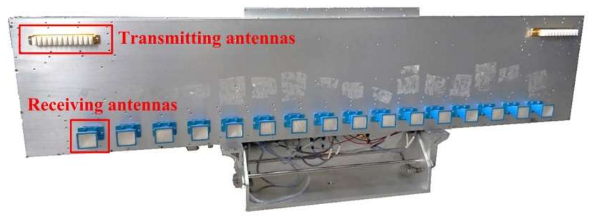
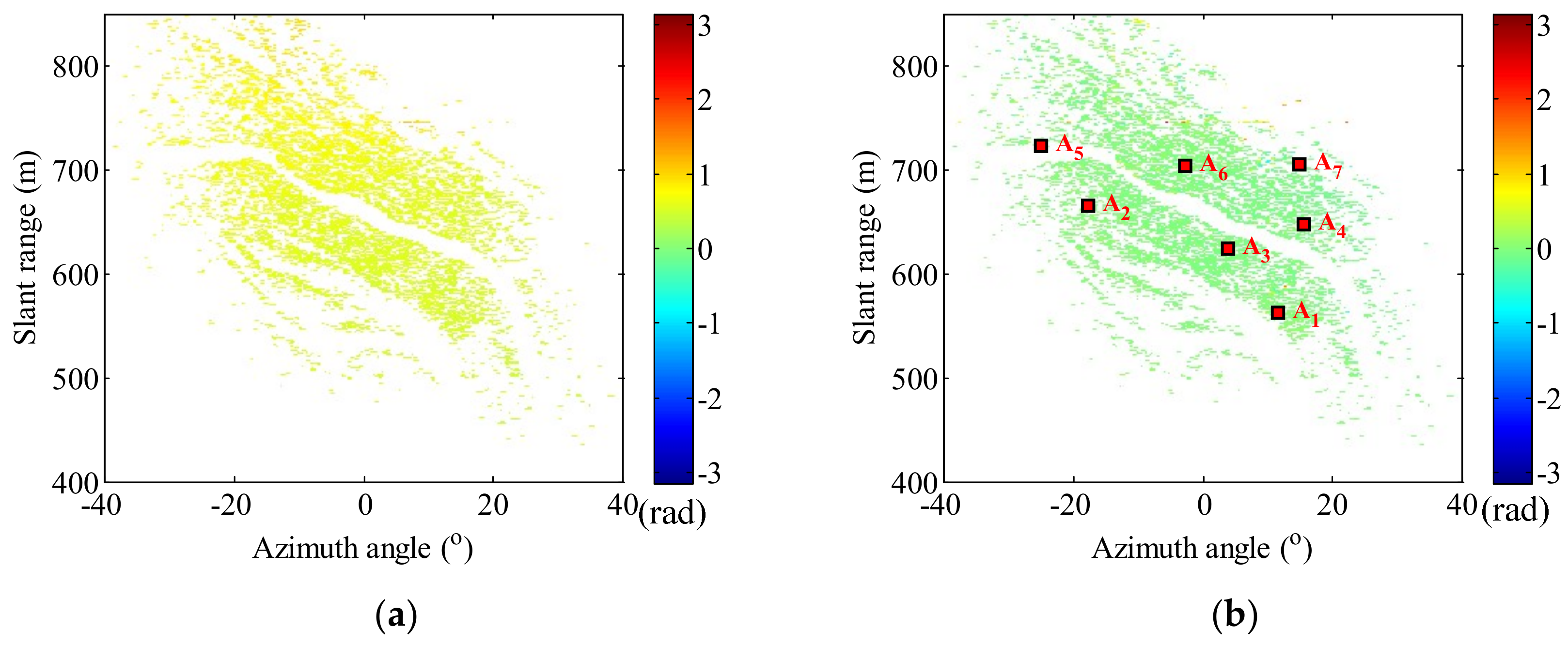
2. Experimental Information
3. Conventional Method
3.1. Method Principle
3.2. Conventional APC
3.3. Problem Analysis
4. Improved Method
- NPS: A PS with a large NP , i.e., an unstable noise-dominant PS.
- DPS: A PS with a small NP but a large DP , i.e., a deformation-dominant PS.
- APS: A PS with a small NP and a small DP , i.e., an atmospheric effect-dominant PS.
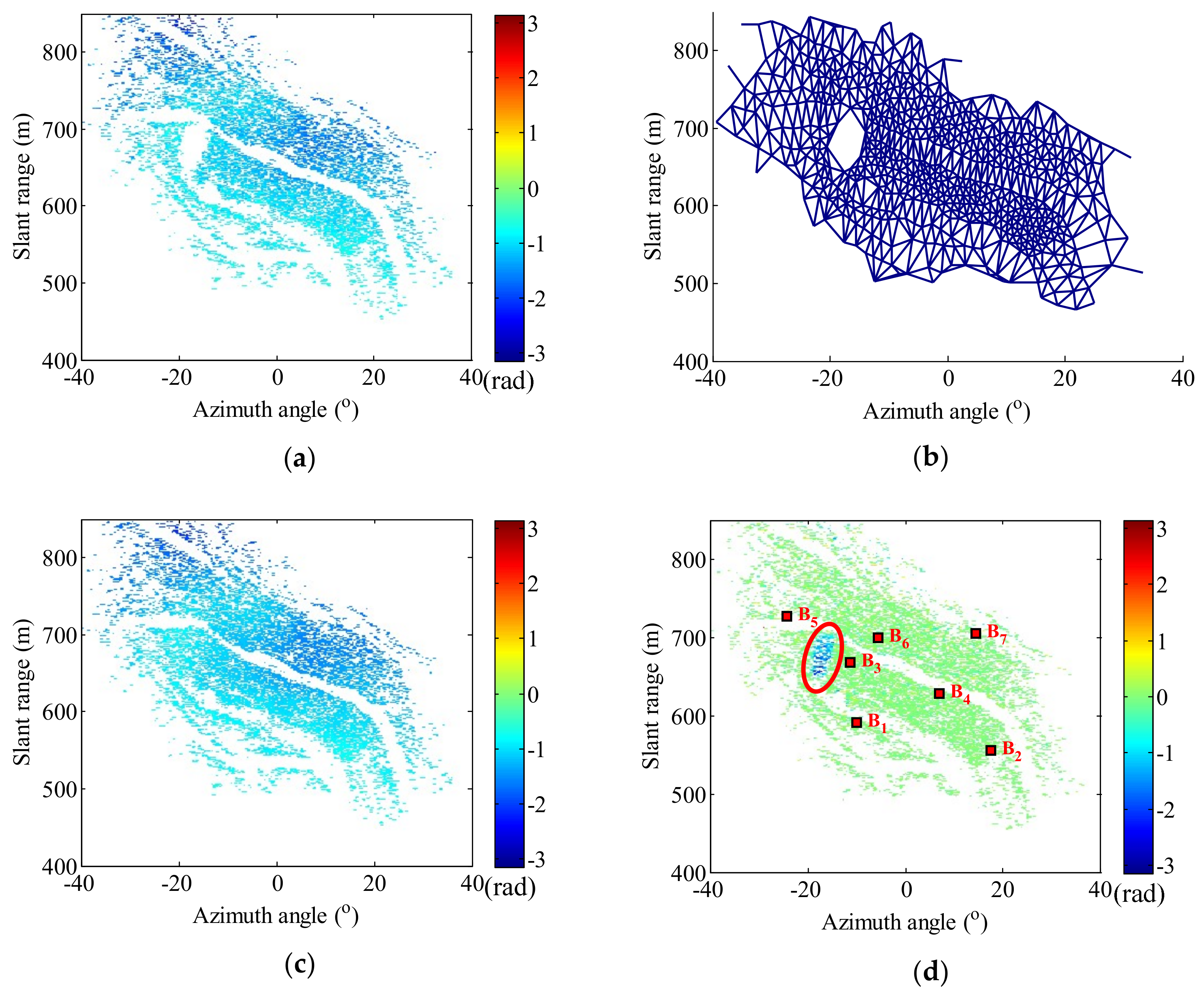
4.1. NPS Rejection
4.2. DPS Rejection
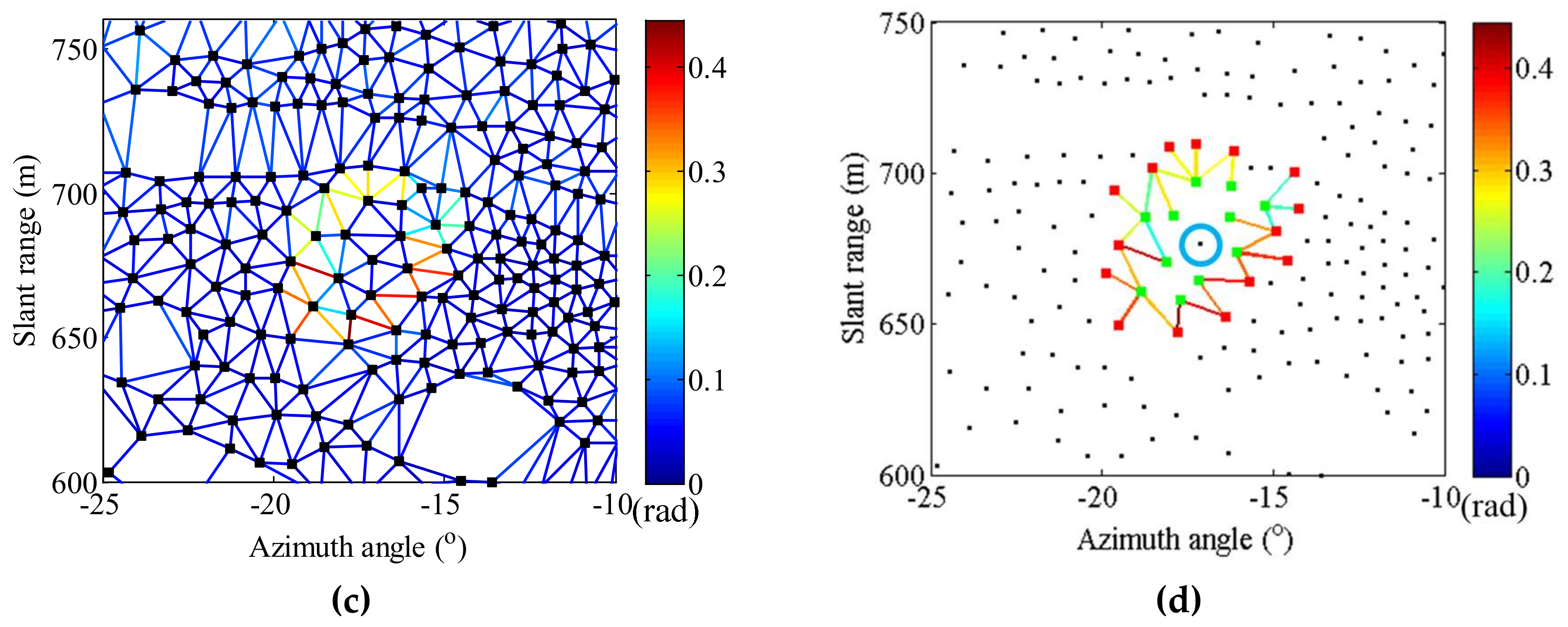
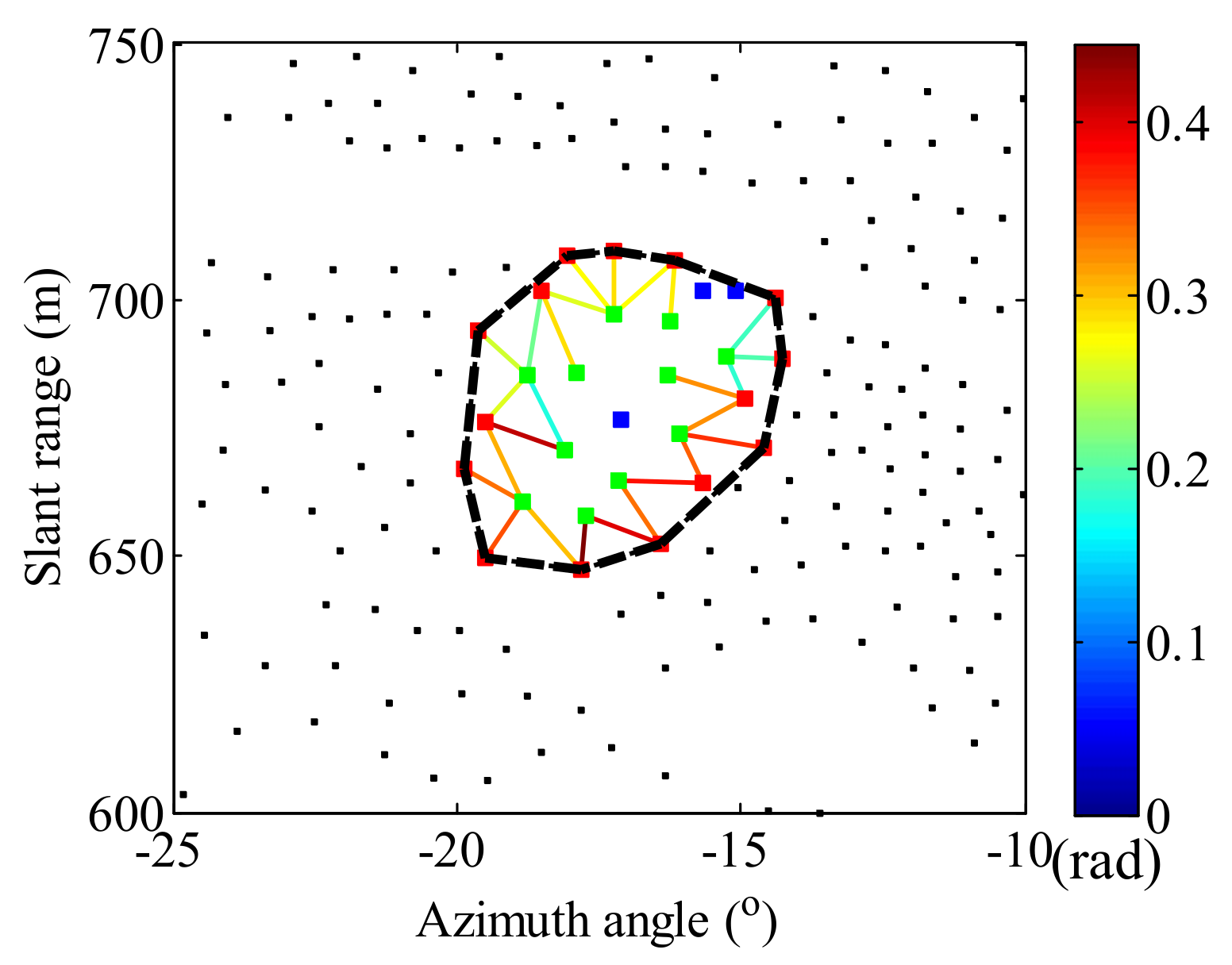
4.2.1. Cluster Partition
- Type I: A cluster with PSs located entirely outside the motional area.
- Type II: A cluster with PSs located entirely inside the motional area.
- Type III: A cluster with PSs located across the motional and motionless areas.
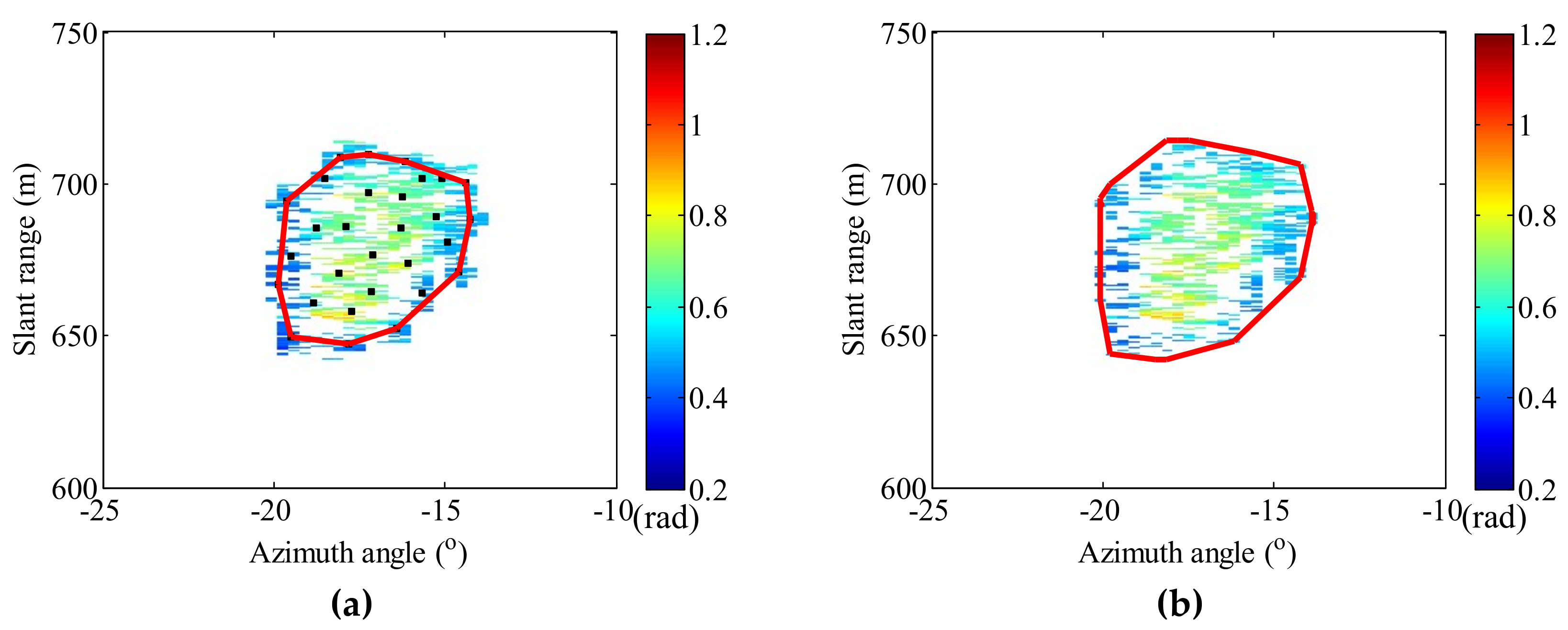
4.2.2. Cluster Selection
- Case 1: If two neighboring clusters both belong to Type I, the AP and the NP are almost eliminated. Therefore, is usually smaller than 0.1 rad.
- Case 2: If two neighboring clusters belong to Type I and Type III, the DP in the difference sequence cannot be neglected and causes to be large.
- Case 3: In other cases, the DP in the difference sequence cannot be quantitatively analyzed, and the value range of is unknown.
4.2.3. DPS Selection
4.3. APS Compensation
5. Experimental Results
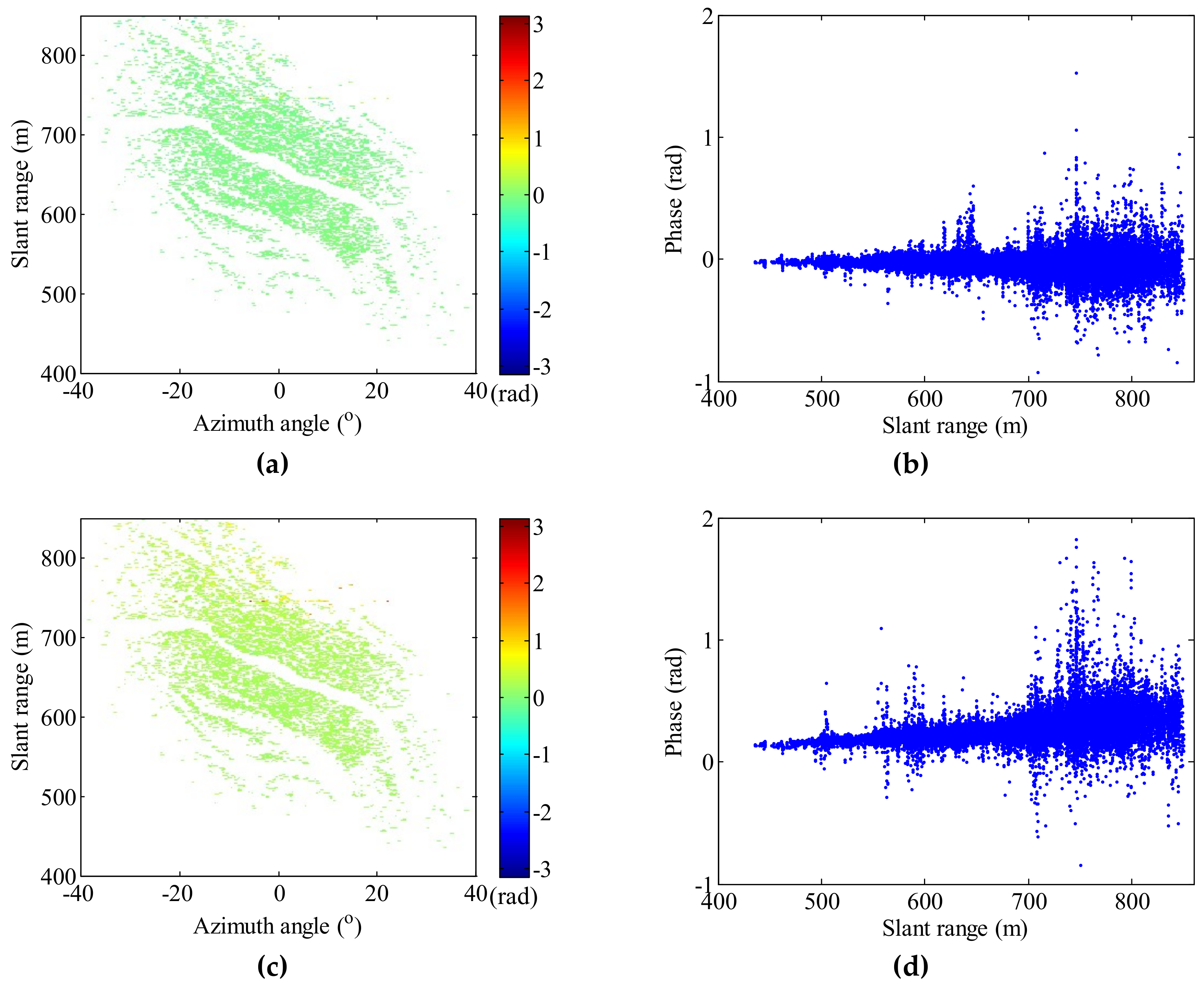
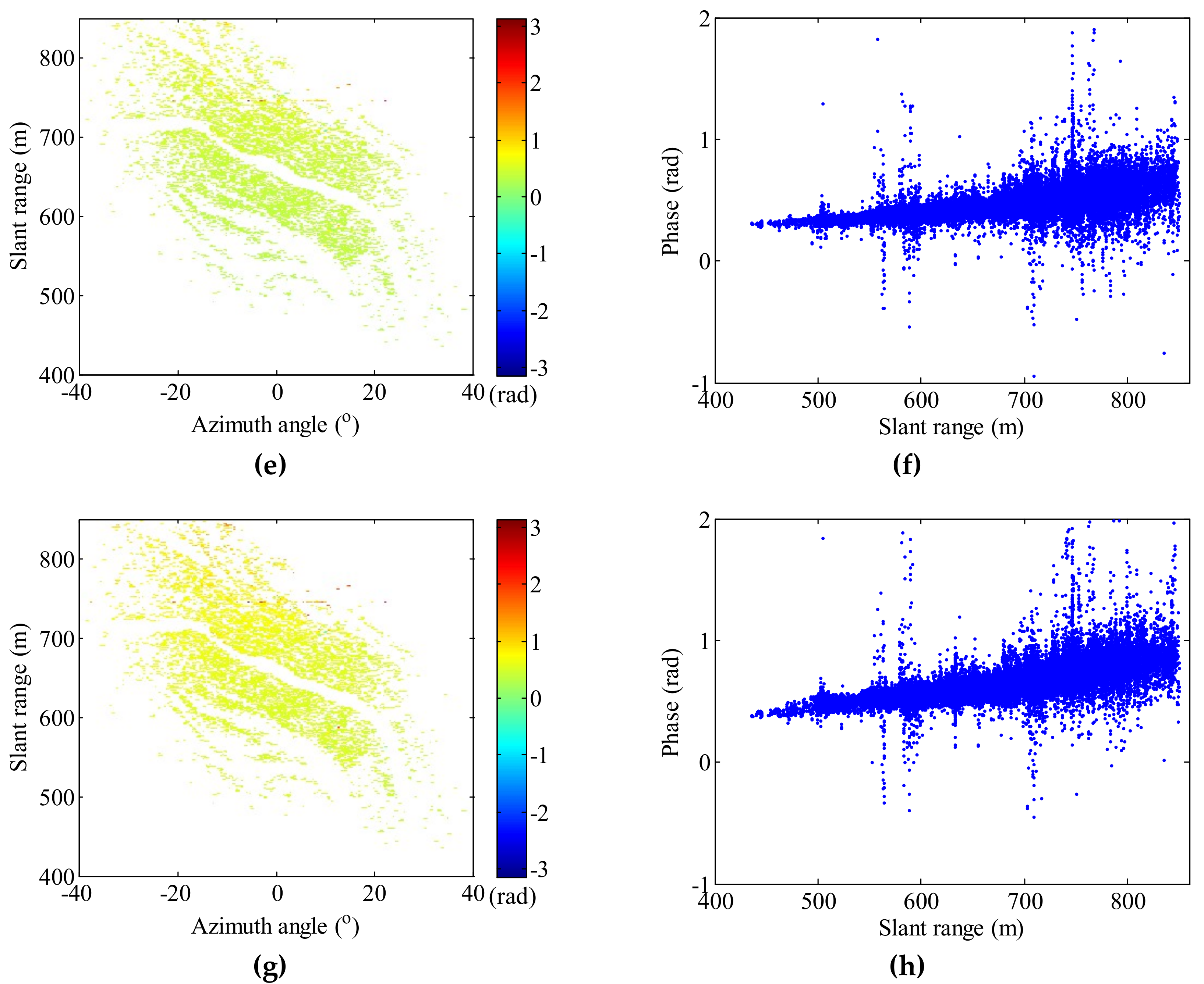
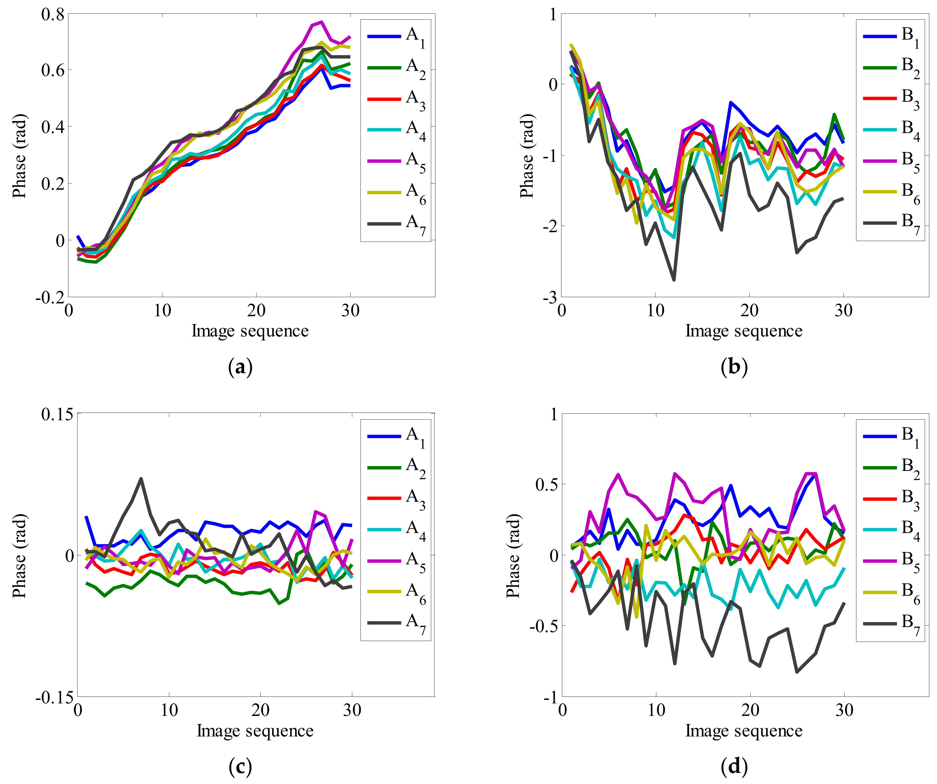
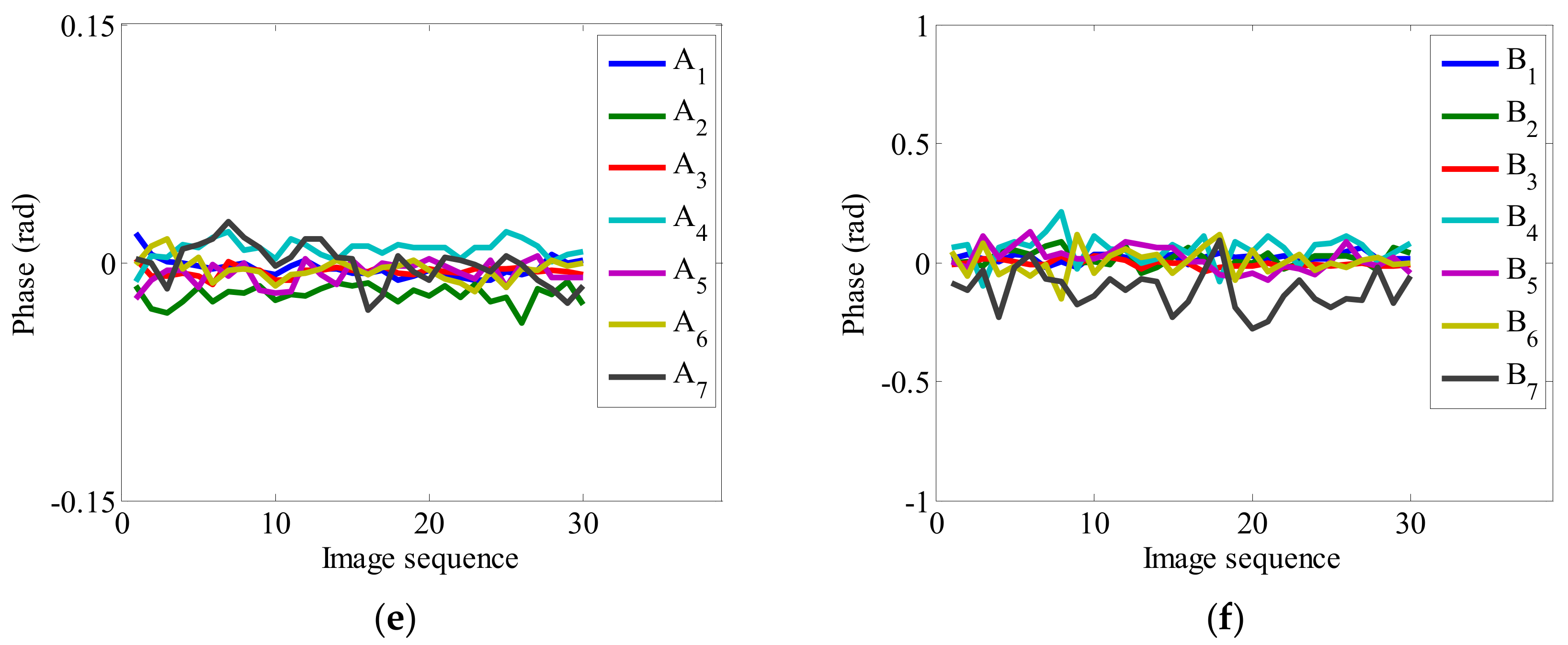
5.1. Short-Term APC
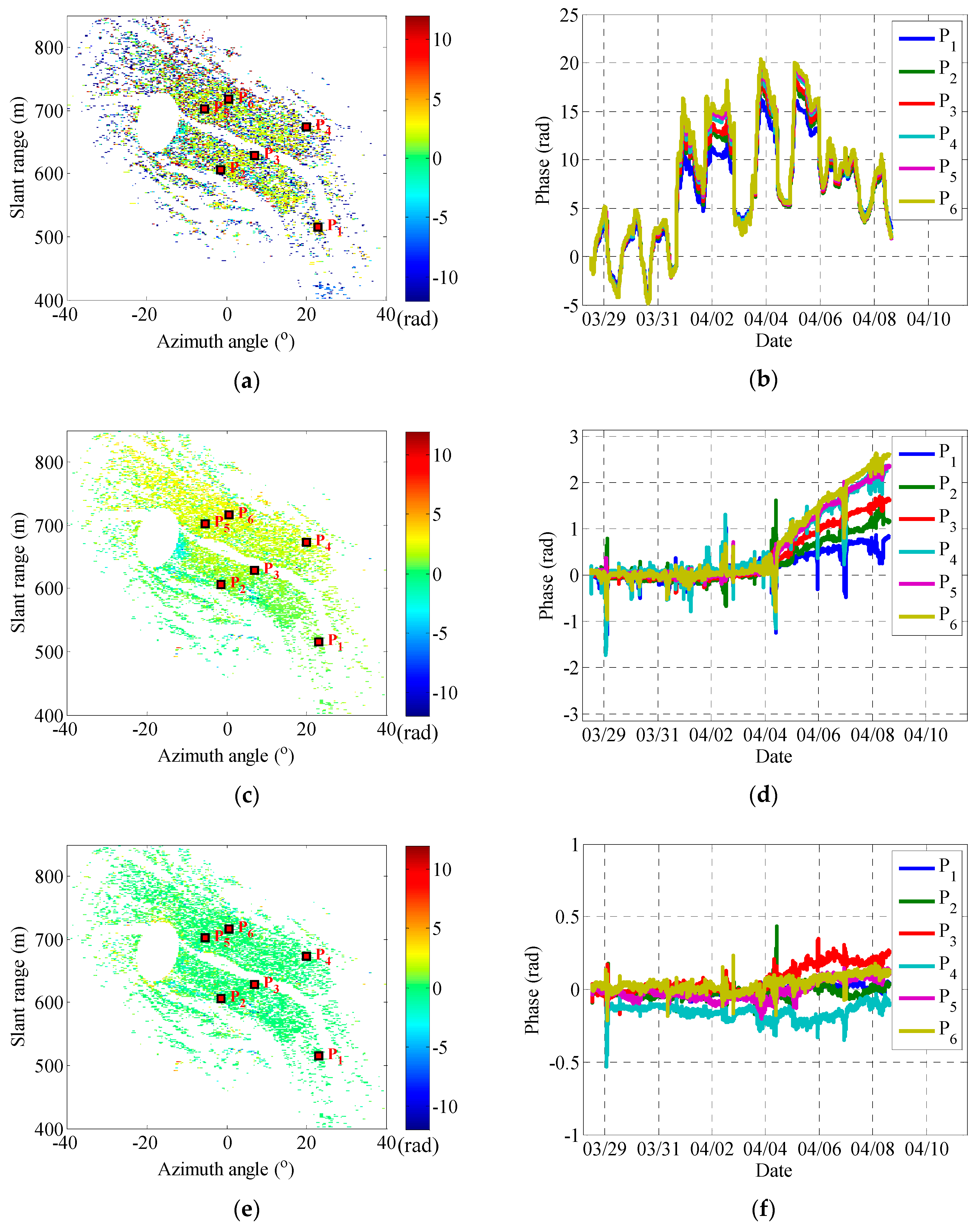
5.2. Long-Term APC
6. Discussion
7. Conclusions
Author Contributions
Funding
Conflicts of Interest
References
- Caduff, R.; Schlunnegger, F.; Kos, A.; Wiesmann, A. A review of terrestrial radar interferometry for measuring surface change in the geosciences. Earth Surf. Process. Landf. 2015, 40, 208–228. [Google Scholar] [CrossRef]
- Pieraccini, M.; Miccinesi, L. Ground-based radar interferometry: A bibliographic review. Remote Sens. 2019, 11, 1029. [Google Scholar] [CrossRef]
- Zheng, W.; Hu, J.; Zhang, W.; Li, Z.; Zhu, J. Potential of geosynchronous SAR interferometric measurements in estimating three-dimensional surface displacements. Sci. China Inf. Sci. 2017, 60, 48–61. [Google Scholar] [CrossRef]
- Hu, C.; Li, Y.; Dong, X.; Cui, C. Optimal 3D deformation measuring in inclined geosynchronous orbit SAR differential interferometry. Sci. China Inf. Sci. 2017, 60, 060303. [Google Scholar] [CrossRef]
- Luzi, G.; Pieraccini, M.; Mecatti, D.; Noferini, L.; Guidi, G.; Moia, F.; Atzeni, C. Ground-based radar interferometry for landslides monitoring: Atmospheric and instrumental decorrelation sources on experimental data. IEEE Trans. Geosci. Remote Sens. 2004, 42, 2454–2466. [Google Scholar] [CrossRef]
- Iannini, L.; Guarnieri, A. Atmospheric phase screen in ground-based radar: Statistics and compensation. IEEE Geosci. Remote Sens. Lett. 2011, 8, 537–541. [Google Scholar] [CrossRef]
- Pipia, L.; Fabregas, X.; Aguasca, A.; Lopez-Martinez, C. Atmospheric artifact compensation in ground-based DInSAR applications. IEEE Geosci. Remote Sens. Lett. 2005, 5, 88–92. [Google Scholar] [CrossRef]
- Noferini, L.; Pieraccini, M.; Mecatti, D.; Luzi, G.; Atzeni, C.; Tamburini, A.; Broccolato, M. Permanent scatter analysis for atmospheric correction in ground-based SAR interferometry. IEEE Trans. Geosci. Remote Sens. 2005, 43, 1459–1471. [Google Scholar] [CrossRef]
- Qiu, Z.; Ma, Y.; Guo, X. Atmospheric phase screen correction in ground-based SAR with PS technique. SpringerPlus 2016, 5, 1594. [Google Scholar] [CrossRef]
- Iglesias, R.; Fabregas, X. Atmospheric phase screen compensation in ground-based SAR with a multiple-regression model over mountainous regions. IEEE Trans. Geosci. Remote Sens. 2014, 52, 2436–2449. [Google Scholar] [CrossRef]
- Hu, C.; Wang, J.; Tian, W.; Zeng, T.; Wang, R. Design and imaging of ground-based multiple-input multiple-output synthetic aperture radar (MIMO-SAR) with non-collinear arrays. Sensors 2017, 17, 598. [Google Scholar] [CrossRef] [PubMed]
- Tarchi, D.; Oliveri, F.; Sammartino, P. MIMO radar and ground-based SAR imaging systems: Equivalent approaches for remote sensing. IEEE Trans. Geosci. Remote Sens. 2013, 51, 425–435. [Google Scholar] [CrossRef]
- Zeng, T.; Mao, C.; Hu, C.; Tian, W. Ground-based SAR wide view angle full field imaging algorithm based on keystone formatting. IEEE J. Sel. Top. Appl. Earth Obs. Remote Sens. 2016, 9, 2160–2170. [Google Scholar] [CrossRef]
- Ferretti, A.; Prati, C.; Rocca, F. Permanent Scatterers in SAR Interferometry. IEEE Trans. Geosci. Remote Sens. 2001, 39, 8–20. [Google Scholar] [CrossRef]
- Hu, C.; Deng, Y.; Tian, W.; Wang, J. A PS processing framework for long-term and real-time GB-SAR monitoring. Int. J. Remote Sen. 2019, 40, 6298–6314. [Google Scholar] [CrossRef]
- Iglesias, R.; Aguasca, A.; Fabregas, X.; Pipia, L.; López-Martínez, C.; Monells, D.; Mallorqui, J.J.; Fabregas, X. Ground-based polarimetric SAR interferometry for the monitoring of terrain displacement phenomena—Part I: Theoretical description. IEEE J. Sel. Top. Appl. Earth Obs. Remote Sens. 2015, 8, 980–993. [Google Scholar] [CrossRef]
- Tian, W.; Zhao, Z.; Hu, C.; Wang, J.; Zeng, T. GB-InSAR-based DEM generation method and precision analysis. Remote Sens. 2019, 11, 997. [Google Scholar] [CrossRef]
- Massonnet, D.; Feigl, L. Radar interferometry and its application to changes in the Earth’s surface. Rev. Geophys. 1998, 36, 441–500. [Google Scholar] [CrossRef]
- Hanssen, R.; Weinreich, I.; Lehner, S.; Stoffelen, A. Tropospheric wind and humidity derived from spaceborne radar intensity and phase observations. Geophys. Res. Lett. 2000, 27, 1699–1702. [Google Scholar] [CrossRef]
- Hanssen, R. Stochastic model for radar interferometry. In Radar Interferometry: Data Interpretation and Error Analysis, 1st ed.; Meer, F., Ed.; Kluwer Academic Publishers: Dordrecht, The Netherlands, 2001; Volume 1, pp. 130–154. [Google Scholar]
- Hu, C.; Zhu, M.; Zeng, T.; Tian, W.; Mao, C. High-Precision deformation monitoring algorithm for GBSAR system: Rail determination phase error compensation. Sci. China Inf. Sci. 2015, 58, 082307. [Google Scholar] [CrossRef]
- Huang, Z.; Sun, J.; Li, Q.; Tan, W.; Huang, P.; Qi, Y. Time- and space-varying atmospheric phase correction in discontinuous ground-based synthetic aperture radar deformation monitoring. Sensors 2018, 18, 3883. [Google Scholar] [CrossRef] [PubMed]
- Tofani, V.; Raspini, F.; Catani, F.; Casagli, N. Persistent scatterer interferometry (PSI) technique for landslide characterization and monitoring. Remote Sens. 2013, 5, 1045–1065. [Google Scholar] [CrossRef]
- Shewchuk, J.R. Delaunay refinement algorithms for triangular mesh generation. Comput. Geom. 2002, 22, 21–74. [Google Scholar] [CrossRef] [Green Version]
- Leva, D.; Nico, G.; Tarchi, D.; Fortuny-Guasch, J.; Sieber, A.J. Temporal analysis of a landslide by means of a ground-based SAR interferometer. IEEE Trans. Geosci. Remote Sens. 2013, 41, 745–752. [Google Scholar] [CrossRef]
- Kanungo, T.; Mount, D.M.; Netanyahu, N.S.; Piatko, C.; Silverman, R.; Wu, A. An efficient k-means clustering algorithm: Analysis and implementation. IEEE Trans. Pattern Anal. Mach. Intell. 2002, 24, 881–892. [Google Scholar] [CrossRef]


| Group | Methods | Deviation/rad | ||||||
|---|---|---|---|---|---|---|---|---|
| A | ||||||||
| Conventional | 0.010 | 0.013 | 0.008 | 0.0120 | 0.016 | 0.010 | 0.026 | |
| Improved | 0.006 | 0.006 | 0.003 | 0.006 | 0.007 | 0.007 | 0.013 | |
| B | ||||||||
| Conventional | 0.132 | 0.117 | 0.137 | 0.100 | 0.194 | 0.138 | 0.224 | |
| Improved | 0.017 | 0.036 | 0.015 | 0.061 | 0.052 | 0.057 | 0.084 | |
© 2019 by the authors. Licensee MDPI, Basel, Switzerland. This article is an open access article distributed under the terms and conditions of the Creative Commons Attribution (CC BY) license (http://creativecommons.org/licenses/by/4.0/).
Share and Cite
Hu, C.; Deng, Y.; Tian, W.; Zhao, Z. A Compensation Method for a Time–Space Variant Atmospheric Phase Applied to Time-Series GB-SAR Images. Remote Sens. 2019, 11, 2350. https://doi.org/10.3390/rs11202350
Hu C, Deng Y, Tian W, Zhao Z. A Compensation Method for a Time–Space Variant Atmospheric Phase Applied to Time-Series GB-SAR Images. Remote Sensing. 2019; 11(20):2350. https://doi.org/10.3390/rs11202350
Chicago/Turabian StyleHu, Cheng, Yunkai Deng, Weiming Tian, and Zheng Zhao. 2019. "A Compensation Method for a Time–Space Variant Atmospheric Phase Applied to Time-Series GB-SAR Images" Remote Sensing 11, no. 20: 2350. https://doi.org/10.3390/rs11202350