Dense Image-Matching via Optical Flow Field Estimation and Fast-Guided Filter Refinement

Abstract

The development of an efficient and robust method for dense image-matching has been a technical challenge due to high variations in illumination and ground features of aerial images of large areas. In this paper, we propose a method for the dense matching of aerial images using an optical flow field and a fast-guided filter. The proposed method utilizes a coarse-to-fine matching strategy for a pixel-wise correspondence search across stereo image pairs. The pyramid Lucas–Kanade (L–K) method is first used to generate a sparse optical flow field within the stereo image pairs, and an adjusted control lattice is then used to derive the multi-level B-spline interpolating function for estimating the dense optical flow field. The dense correspondence is subsequently refined through a combination of a novel cross-region-based voting process and fast guided filtering. The performance of the proposed method was evaluated on three bases, namely, the matching accuracy, the matching success rate, and the matching efficiency. The evaluative experiments were performed using sets of unmanned aerial vehicle (UAV) images and aerial digital mapping camera (DMC) images. The results showed that the proposed method afforded the root mean square error (RMSE) of the reprojection errors better than ±0.5 pixels in image, and a height accuracy within ±2.5 GSD (ground sampling distance) from the ground. The method was further compared with the state-of-the-art commercial software SURE and confirmed to deliver more complete matches for images with poor-texture areas, the matching success rate of the proposed method is higher than 97% while SURE is 96%, and there is 47% higher matching efficiency. This demonstrates the superior applicability of the proposed method to aerial image-based dense matching with poor texture regions.

1. Introduction

Dense image-matching uses acquisition homonymous points for each pixel in the overlap of stereo image pairs. It is essential for photogrammetric applications, including digital surface model (DSM) generation, three-dimensional (3D) reconstruction, and object detection and recognition [1]. Given a pair of stereo images and corresponding camera parameters, the goal of dense image-matching is to generate the 3D point clouds of the overlap area between the stereo image pairs. Over the last few decades, dense image-matching has attracted extensive interest in the fields of photogrammetry and computer vision, and substantial developmental progress has been achieved [1,2]. Available dense image-matching algorithms can be divided into two types, namely, stereo-matching algorithms and multi-view stereo-matching algorithms. The stereo-matching strategy is mostly used in the field of photogrammetry, with the correspondences determined by taking into consideration the geometric and radiometric constraints between stereo image pairs [3]. Based on the employed cost-aggregation method [4], dense image-matching can also be divided into two categories, namely, those that utilize local algorithms [5,6,7,8] and global algorithms [9,10,11,12,13], respectively. A local algorithm determines the correspondences by calculating the matching costs between the selected point and its local surrounding, and then uses the winner-takes-all (WTA) strategy to select the point with the minimum matching cost as the final corresponding point [5,14]. Because a local algorithm only uses part of the local neighbors for its calculations, it affords low computational complexity and redundancy. However, it may quickly become stuck in local optima, which would cause the matching result not to match the actual topography. Conversely, a global algorithm globally optimizes its final matching result using a pixel-based or object-based cost function optimized by the energy function through graph cuts or a Markov random field (MRF) method [13,15]. Because this type of algorithm considers the entire image, its matching precision is higher than that of a local algorithm. However, a global algorithm has the disadvantage of involving a substantial amount of redundant computations, which result in a low matching efficiency. Hirschmüller [16] proposed a semi-global matching (SGM) algorithm with improved computational efficiency based on multi-directional dynamic programming. Compared with traditional global algorithms and local algorithms, the SGM algorithm considers only the non-occluded points during the image-matching process, and this further improves both the matching accuracy and efficiency. Whereas the stereo dense matching method has the advantages highlighted above, it only considers the information contained in two images, which causes its matching results to be susceptible to occlusion and noise [17]. By the comprehensive study of SGM, Rothermel et al. improved the SGM algorithm with a hierarchical approach to initialize and refine the matching cost, and thereby the improved SGM methods can handle the large image as photogrammetric applications [18].

Multi-view stereo matching has always been a hot topic in the field of computer vision [19]. Because geometrical relationships and redundant information are considered during the matching process, the robustness of the results of multi-view stereo matching against occlusion and noise is higher than those of stereo matching. Multi-view stereo matching methods can be categorized as those that utilize voxel-based, polygonal mesh-based, depth map-based, and patch-based matching algorithms, respectively. In methods that utilize voxel-based matching algorithms, the need to consider the grid size of the voxel in the matching process causes inadequacy when applied to large-scene images, resulting in not suitable for photogrammetry [20,21]. A polygonal mesh-based algorithm significantly depends on a prior input, and this causes inflexibility [22]. Although a depth map-based approach is more flexible, the utilized depth map is noisy and achieving efficiency of the algorithm requires a series of post-processing measures such as fusion, de-noising, and filtering of the depth map to eliminate the redundant computations that the noise would otherwise cause [23,24]. By identifying sparse feature points in the image, the patch-based matching method creates several small feature patch sets and achieves dense image-matching effects through matching propagation [25,26]. The patch-based multi-view stereo (PMVS) presented by Furukawa and Ponce is widely used in state-of-the-art algorithms. Because the PMVS does not require any prior knowledge or initial value and can be applied to the 3D reconstruction of large-scale images, it is extensively used for unmanned aerial vehicle (UAV)-based low-altitude 3D photogrammetric measurements [27]. Ai et al. fed high-precision sparse matching points into PMVS as seed points to obtain dense point clouds [28], and thereby significantly improve the matching efficiency of the software. Shao et al. used the matching result of PMVS as the initial values for creating expanded patch sets [29], with the correspondences adjusted by least-squares refinement and a patch-based multi-photo geometrical constrained (MPGC) method [30]. This process enables the achievement of point clouds that are much denser and more robust against occlusion.

To address the issues of stereo-matching methods, the high-matching computational redundancy in a fixed matching window size and the poor matching resulting in areas of sharp depth discontinuities, we developed a coarse-to-fine dense image-matching method that utilizes an optical flow field estimation and a fast guided filter refinement. The performance of this proposed optical flow field-based dense image-matching method (OFFDIM) was qualitatively and quantitatively evaluated on three bases, namely, the visual effect on point clouds, the matching success rate, and the matching accuracy. The practical applicability of the method to the dense matching of aerial images was also confirmed. Comparison of the proposed method with the commercial software SURE [31] further demonstrated the potential of the former for the acquisition of high-precision dense 3D point clouds using aerial and UAV images.

The main contributions of this paper may be summarized as follows:

(1)

A novel coarse-to-fine dense aerial image-matching strategy is proposed.

(2)

The B-spline approximation (BA) algorithm is improved into a triangulation-based multi-level B-spline approximation (TMBA) algorithm in order to avoid the estimated dense optical flow field over smooth.

(3)

A fast guided filter based refinement method is introduced to achieve a better matching completeness in poor texture and sharp depth discontinuity region.

2. Methodology

2.1. Complete Procedure

The flowchart of the proposed dense image-matching method is presented in Figure 1. The input data for the OFFDIM is a pair of raw images and the corresponding camera parameters (interior and exterior orientation elements). The OFFDIM method involves four steps: (1) preprocessing, (2) coarse-matching, (3) fine-matching, and (4) 3D point cloud generation. In the first step, some highly-accurate and uniform image tie points are extracted by the feature-based image-matching method. In this paper the scale invariant feature transform (SIFT) feature matching is utilized for tie point extracting, and a least square image-matching is adopted for improving the matching accuracy [32]. The accurate tie points are then used for relative orientation, overlap area determination, and epipolar image generation. The second step involves the use of the optical flow field for coarse-matching. The sparse optical flow field is calculated by the feature-based pyramid Lucas–Kanade (L–K) method, and the proposed triangulation-based multi-level B-spline approximation (TMBA) method is then used to estimate the dense optical flow field. Based on the dense optical flow field, the pixel-wised movement between raw stereo image pairs can be used to calculate the dense correspondence. In the third step, the coarse-matching results for the raw image pairs are projected onto the corresponding epipolar image pairs for initial disparity calculation. Subsequently, the proposed cross region-based voting algorithm is used to determine the valid disparity search range for each pixel in the overlapped area. Cost aggregation based on a fast-guided image filter is then used to refine the disparity map. Finally, the coordinates of the initial corresponding point pairs are accurately corrected based on the geometric relationship between the pixel coordinates of the epipolar image and those of the original image. In the foregoing procedure, the dense correspondence image coordinates and the corresponding camera parameters are adequate and the dual-image spatial intersection principle [33] is used for the point-wised calculation of the 3D ground coordinates of the homonymous points.

Because the preprocessing and 3D point cloud generation steps utilize widely used techniques, they are not discussed in detail here. The present focus would be an elaboration of the key improvements of the coarse- and fine-matching strategies. Section 2.2 introduces the proposed TMBA method for estimating the dense optical flow field, while Section 2.3 describes the cross region-based voting and fast guided filter-based disparity map refinement for the coarse-matching point refinement.

2.2. Optical Flow Field-Based Coarse-Matching Method

The purpose of the coarse-matching step is the provision of an initial value of the pixel-wised correspondence for guiding the fine-matching. The initial value enables reduction of the search range for generating the disparity map. The use of an optical flow field facilitates the process and the technique is widely used in object-detection applications owing to its high speed and pixel-based motion tracks. Most available real-time optical flow methods can only be used to generate sparse optical flow fields.

Dense optical flow methods always utilize optimal global energy functions and involve extremely complex computations. Meanwhile, traditional sparse optical flow methods such as L–K methods [34] are never successful when applied to large pixel motions. Incidentally, image sequences acquired by aerial photography or low-altitude UAV photography always contain larger motions. To obtain a better initial value, we first used a pyramid L–K method to calculate the sparse optical flow field based on the preprocessing-acquired tie points. TMBA was then used to estimate the dense optical flow field.

After obtaining the sparse optical flow fields, the estimation of the dense optical flow field in the overlapping region of a stereo image pair can be regarded as a process of interpolating unknown points from the discrete point set. If a pixel corresponds to a static ground object, the change of the optical flow field in the ground object region should be continuous and smooth. Because the obtained sparse optical flow field may not lie on an integer pixel grid, its distribution may be non-uniform. The TMBA method proposed in this paper is used for the estimation of the dense optical flow field. The B-spline approximation (BA) method is briefly introduced in Section 2.2.1, the proposed triangulation-based B-spline approximation (TBA) procedure is presented in Section 2.2.2, while the proposed TMBA is described in Section 2.2.3.

2.2.1. B-Spline Approximation (BA) for Dense Optical Flow-Field Estimation

Generally, within an overlapping region of a reference image, a uniform tensor grid covering the region is constructed by the BA method and used to store the coefficients of each control point for calculation of the interpolation function. Assuming that $\Omega$ denotes a rectangular region of size $m\times n$, and $\Phi$ is the control lattice stretching over the grid points within $\mathit{\Omega }$, of size $(m+3)\times (n+3)$. Then, $\left(x,y\right)\in \Omega$ would hold for the discrete point set $\mathit{Q}=\left\{\left(x,y,\overrightarrow{o}\right)\right\}$, where $\left(x,y\right)$ denotes the pixel coordinates in the left raw image, and $\overrightarrow{o}=[x-x^{\prime },\hspace{0.17em}y-y^{\prime }]=[o_x,o_y]$ is the 2D optical flow vector between the pixel $\left(x,y\right)$ in the left raw image and its corresponding pixel $\left(x\prime ,y\prime \right)$ in the right raw image. If ${\varphi }_{ij}$ is the coefficient of the control point with coordinates in the control lattice, the fitting function for calculating the optical flow can be defined in terms of the control lattice as follows [34]:

$$o_r(x,y)={\displaystyle \sum _{k=0}^3{\displaystyle \sum _{l=0}^3{B}_k(s)B_l(t)}}{\phi }_{(i+k)(j+l)},\hspace{1em}(r=x,y)$$

(1)

where $i=⎣x⎦$, $j=⎣y⎦$, $s=x-⎣x⎦$, $t=y-⎣y⎦$, $B_k$, and $B_l$ are uniform cubic B-spline basis functions defined as follows [34]:

$$B_i(t)=\{\begin{array}{l}{(1-t)}^3/6,\hspace{1em}\hspace{1em}\hspace{1em}i=0\\ (3t^3-6t^2+4)/6,\hspace{1em}i=1\\ (-3t^3-3t^2+3t+1)/6,\hspace{1em}i=2\\ t^3/6,\hspace{1em}\hspace{1em}\hspace{1em}\hspace{1em}\hspace{1em}\hspace{1em}\hspace{1em}\hspace{1em}\hspace{0.17em}i=3\end{array}$$

(2)

where $t\in \left[0,1\right]$.

The cubic uniform B-spline basis function is used to weight the fitting contribution by calculating the distance between each control point and the point $\left(x,y\right)$. The entire interpolation problem can, therefore, be expressed by finding the best control point lattice $\mathit{\Phi }$ that affords optimal fitting to the given discrete point set $\mathit{Q}$. Lee et al. noted that when a control point on the control lattice is only related to one point $\left(x,y,\overrightarrow{o}\right)$ in the discrete point set $\mathit{Q}$, ${\varphi }_{ij}$ can be obtained as follows [34]:

$${\phi }_{ij}=\frac{B_i(s)B_j(t)o_r}{{\displaystyle \sum _{k=0}^3{\displaystyle \sum _{l=0}^3{(B_k(s)B_l(t))}^2}}},\hspace{1em}(r=x,y)$$

(3)

When ${\varphi }_{ij}$ is related to none of the points in the discrete point set $\mathit{Q}$, its value is set to 0. In actual photogrammetric applications, the control point is always not related to any sparse optical flow point within the boundaries of the image overlapping region and the featureless area. Hence, in the BA method, the $\varphi$ values of the control points are set to 0, resulting in the final estimation tending to 0 and being over-smooth. With regard to the estimation of the dense optical flow field, this is unreasonable. A control lattice generation approach is, therefore, proposed in this paper to enable better determination of the interpolating function using Delaunay triangulation-based linear interpolation.

2.2.2. Triangulation-Based B-Spline Approximation (TBA) Procedure

The procedure of the triangulation BA algorithm (TBA) is as follows:

(1)

The BA method is used to calculate the control lattice $\mathit{\Phi }$ from the discrete optical flow point set $\mathit{Q}$.

(2)

Delaunay triangulation is performed on the sparse optical flow points set $\mathit{Q}$ in the image coordinate system, and a linear interpolation function is constructed within each triangle to calculate the optical flow $\overrightarrow{o}\prime$ using Equation (4).

$${\overrightarrow{o}}^{\prime }=\alpha {\overrightarrow{o}}_1+\beta {\overrightarrow{o}}_2+\gamma {\overrightarrow{o}}_3$$

(4)

where ${\overrightarrow{o}}_1$, ${\overrightarrow{o}}_2$ and ${\overrightarrow{o}}_3$ are optical flow values corresponding to the three vertices of the triangle; $\alpha , \beta \mathrm{and} \gamma$ are weighted parameters determined by the Euclidean distance between the selected points to the three vertices of the triangle, and $\alpha +\beta +\gamma =1$.

(3)

Equation (3) is used to calculate the control lattice $\mathit{\Phi }\prime$ using obtained ${\overrightarrow{o}}^{\prime }$ in step 2).

(4)

The points in control lattice $\mathit{\Phi }\prime$ that fall within a Delaunay triangular grid region are selected and their total number n is calculated.

(5)

The selected points are used to calculate the adjusted distance $d_r=\frac{1}{n}{\displaystyle \sum _{i=1}^n(o_r-{o^{\prime }}_r)},\hspace{1em}(r=x,y)$.

(6)

The adjusted control lattice $\mathit{\Phi }$ is calculated by substituting $o_r-\delta d_r,(r=x,y)$ for $o_r$ in Equation (3), here,$\delta$ is an experienced weighting value that is generally set to 0.5.

2.2.3. Triangulation-Based Multi-Level B-Spline Approximation (TMBA) Strategy for Dense Optical Flow Field Estimation

To achieve a more accurate approximation, we used a hierarchy of the control lattice to estimate the dense optical flow field. Assuming that ${\mathit{\Phi }}_0,{\mathit{\Phi }}_1,\dots ,{\mathit{\Phi }}_{\mathrm{k}}$ overlay the domain $\Omega$ and the spacing of the control points in ${\mathit{\Phi }}_{\mathrm{k}}$ is half of that in ${\mathit{\Phi }}_{\mathrm{k}-1}$, the control points at (i, j) in the control lattice ${\mathit{\Phi }}_0$ will coincide with the position (2i, 2j) in ${\mathit{\Phi }}_1$. At first, the TBA is applied to the discrete optical flow point set $\mathit{Q}$, the coarsest control lattice ${\mathit{\Phi }}_0$, and the estimation function $o_r^{(0)}(x,y),(r=x,y)$, can be calculated. For each point $\left(x,y,\overrightarrow{o}\right)$ in $\mathit{Q}$, by applying the estimation function $o_r^{(0)}(x,y),(r=x,y)$, the estimated optical flow value is presented as ${\overrightarrow{o}}_0=[o_x^{(0)}(x,y),o_y^{(0)}(x,y)]$ the displacement of the estimated optical flow value and the ground truth value can be calculated as $\Delta \overrightarrow{o}$ = $\overrightarrow{o}-{\overrightarrow{o}}_0$. The next control lattice ${\mathit{\Phi }}_1$ is then used to obtain an estimation function $o_r^{(1)}(x,y),(r=x,y)$ to approximate the difference in the optical flow field on ${\mathit{Q}}_1=\left\{\left(x,y,\Delta \overrightarrow{o}\right)\right\}$. Through this procedure, the estimation function $o_r^{(i)}(x,y),(r=x,y)$ will produce a smaller difference between the estimated optical flow field and the sparse control points-generated optical flow field. Assuming that the hierarchy is of level k, the final approximation function can be derived as follows:

$$Q_r={\displaystyle \sum _{i=0}^k{Q}_r^{(i)}}(x,y),\hspace{1em}\hspace{1em}(r=x,y)$$

(5)

where k is the level of the hierarchy, usually, k is set to 8.

The dense optical flow value of each pixel in the overlapping region of the stereo image pairs can be estimated using Equation (5) as $\overrightarrow{o}=[o_x(x,y),o_y(x,y)]$.

2.3. Refinement of Coarse-Matching Point Using Fast-Guided Filter

After the estimation of the dense optical flow field, the coarse-matching correspondences are obtained. The coarse-matching result is then used as an initial value for fine-matching. In this novel pixel-wise fine-matching process, the approximate coordinates of the corresponding points extracted by the dense optical flow field are first transformed into the coordinates of the epipolar images and used to determine the valid disparities through cross-region-based voting. The census cost of each valid disparity is then calculated, followed by cost aggregation using the fast-guided filter (FGF) [35]. Afterward, a WTA strategy is used to select the optimal disparity corresponding to the lowest cost among the valid disparities of a pixel, and a disparity map is generated. Finally, the initial matched points are refined with the aid of the known geometric relationship between the disparity map and the epipolar image.

The overall fine-matching procedure thus consists of cost calculation, candidate disparity determination, cost aggregation, and disparity refinement. Below is a detailed description of each step.

2.3.1. Cost Volume Calculation

Because aerial images always contain geometric and radiometric distortions, some widely used costs such as the sum of absolute differences (SAD) [4] and sum of squared differences (SSD) [35,36] are unable to correctly indicate similarities because of their sensitivity to noise. To solve this problem, we use census transform to deal with illumination changes and noise. A detailed description of census transform is available in the work of Zabih [34]. After census transformation, the effects of the overall linear radiometric distortion and local irregularities in a search window are reduced by mapping the intensity differences between the central pixel and its neighbor pixels using their binary values. By this means, the census cost is adopted as the cost volume.

There are two steps in the cost-calculation procedure. In the search and reference windows, the intensity differences between the central pixel and its neighboring pixels are respectively encoded into binary bit strings through census transformation. The costs are then obtained by calculating the Hamming distance between strings using Equation (6) [37]:

$$C_{il}=hamdist(Censu{s}_r(I(i)),\hspace{0.17em}Censu{s}_r(I^{\prime }(i_l)))$$

(6)

where $C_{il}$ is the raw cost for pixel i in the left image with disparity l; $Censu{s}_r(\ast )$ is an r×r Census feature; I and I′ are respectively the left and right grayscale images; i and i_l are, respectively, the pixel i in the left image and its corresponding pixel with disparity l in the right image; and $hamdist\hspace{0.17em}(\ast ,\ast )$ indicates hamming distance.

2.3.2. Cross Region-Based Disparity Range Voting

The real world is composed of complex spatial structures. Thus, the distribution of disparities is not a simple uniform distribution [38]. Furthermore, treating the selected probabilities of all the possible disparities as being equal makes the algorithm computationally redundant. Based on the epipolar image and the coarse-matching results, we propose a cross region-based voting algorithm for determining the valid disparity search range. In real-world scenarios, there are always depth discontinuities at an object boundary, and an object usually has similar color information within a spatial area. Based on this assumption, we used a color factor and spatial factor to define the cross-region of a selected pixel. The following constraints were imposed on the cross-region of a pixel p in the epipolar image:

(1)

${\mathrm{D}}_c\left(p,q\right)<{\tau }_1$ and ${\mathrm{D}}_c\left(p,q\mp \left(0,1\right) \mathrm{or} (1,0\right)<{\tau }_2$

where ${ \mathrm{D}}_c\left(p,q\right)$ is the color difference factor between pixels p and q, defined as ${\mathrm{D}}_c\left(p,q\right)=\underset{n=R,G,B}{\max }\left|I_n\left(p\right)-I_n\left(q\right)\right|$, and ${\tau }_1 and {\tau }_2$ are predefined constants for avoiding a large color difference between p and q.

(2)

${\mathrm{D}}_s\left(p,q\right)<$ L

where ${\mathrm{D}}_s\left(p,q\right)$ is the euclidean distance between p and q in the coordinate system of the epipolar image. L is the predefined constant to limit the spatial distance between p and q.

Usually, we set ${\tau }_1$ = 10, and L = 20. After determining the cross-region of each pixel in the epipolar image, a histogram with a bin size of 1 is used to sort the frequency of the disparity value in the cross-region. The top 50% disparities are then selected as the valid disparities to limit the disparity search range. Figure 2 illustrates the process. First, the vertical range of p is searched to determine the initial vertical range of the cross-region, and then, for each pixel q in the vertical region, the horizontal region is constructed by expanding the vertical region. The coarse-matching result is subsequently assigned to the constructed cross-region to build the voting map. The yellow square in Figure 2b represents the selected pixel, and the number in each square is the coarse-matching disparity of the corresponding pixel.

2.3.3. Cost Aggregation Using Fast-Guided Filter

The information contained in a single pixel is often inadequate for global optimal matching. To address this issue, local stereo-matching methods are often used to aggregate the matching costs. The essence of the cost aggregation is a least-squares adjustment of the costs in a matching window. One of the most-used box filters assumes constant disparity in a window in performing the least-squares adjustment. This paper uses a fast-guided filter to aggregate the census costs.

A left epipolar image and an image composed of costs are used as the guided image and the reference image, respectively. The filtered costs are calculated using Equation (7) [39] and parameters obtained based on the mean and variance of the intensity in a matching window.

$$C_{il}^{\prime }={\displaystyle \sum _j{W}_{ij}(I)}{C}_{jl}$$

(7)

where $C_{il}^{\prime }$ is a filtered cost; I is the guided image; and $W_{ij}$ is the weight of pixel j relative to the central pixel i, given by [39]

$$W_{ij}=\frac{1}{|\omega {|}^2}{\displaystyle \sum _{k:(i,j)\in {\omega }_k}(1+\frac{(I_i-{\mu }_k)(I_j-{\mu }_k)}{{\sigma }_k^2+\epsilon }})$$

(8)

where $\omega$ is a normalization factor; I_i and I_j are respectively the intensities of pixels i and j in the guided image, ${\mu }_k$ and ${\sigma }_k^2$ are respectively the mean and variance of the intensity in the matching window k of the guided image, and $\epsilon$ is the smoothness coefficient.

It can be deduced from Equation (8) that the weight of a pixel in a matching window is determined by the spatial distance and consistency of the intensity. A large spatial distance between a selected pixel and the central pixel in a matching window would produce a small weight. Conversely, the high-intensity similarity between the selected pixel and the central pixel in a matching window produces a large weight. In other words, a pixel close to the center of the matching window and with an intensity similar to that of the central pixel would have a large weight.

The output of the guided filter is a linear combination of the intensities of the guide images [39]:

$$q_i=a_k{I}_i+b_k,\hspace{1em}\hspace{1em}i\in {\omega }_k$$

(9)

where $q_i$ and $I_i$ are, respectively, the grayscale intensity values of pixel i in the output image and guided image, and $a_k,b_k$ are, respectively, parameters calculated using the reference image [39]:

$$\begin{array}{l}{a}_k=\frac{\frac{1}{n}{\displaystyle \sum _{i\in {\omega }_k}{I}_i{p}_i-{\mu }_k{\overline{p}}_k}}{{\sigma }_k^2+\epsilon }\\ b_k={\overline{p}}_k-a_k{\mu }_k\end{array}$$

(10)

where n is the number of pixels in the matching window ${\omega }_k$, and ${\overline{p}}_k$ is the mean of the grayscale pixels intensities of the reference image in ${\omega }_k$.

2.3.4. Refinement of Disparity Map and Coarse-Matching Points

After calculating the parameters of a pixel, a box filter is used to smoothen the results. The grayscale intensities of an output image represent a linear transformation of the grayscale intensities of the guided image. Therefore, the guided filter can be used to well preserve the edges of the original image in the output image. According to He [40], the parameters of the guided image filter can first be calculated from down-sampled images, and the results can then be up-sampled for each pixel in the corresponding original images.

It is also noteworthy that filtered costs are less affected by noise and authentically reflect the disparity changes in the original images. Based on filtered costs, a WTA strategy can be used to select the disparity corresponding to the lowest cost from among valid disparities to generate a fine-matched disparity map. After the acquisition of the disparity map, the popular left–right consistency check can be used to identify mismatched pixels. The disparity of a mismatched pixel can also be determined based on the nearest reliable pixel. A weighted median filter is then used to refine the disparity map by removing the peaks and noise.

With the aid of the refined disparity map and the initial pixel coordinates of the epipolar images, the refined pixel coordinates of the coarse-matched points can be obtained as follows:

$$\{\begin{array}{l}{x}_{refined}^l=x_{initial}^l\\ y_{refined}^l=y_{initial}^l\\ x_{refined}^r=x_{refined}^l-\mathrm{disp}(x_{initial}^l,y_{initial}^l)\\ y_{refined}^r=\{\begin{array}{c}{y}_{initial}^r,\hspace{0.17em}\hspace{1em}\left|y_{initial}^r-y_{refined}^l\right|<\tau \hspace{0.17em}\hspace{0.17em}\\ y_{refined}^l,\hspace{0.17em}\hspace{0.17em}\hspace{0.17em}\hspace{0.17em}\mathrm{otherwise}\hspace{1em}\hspace{1em}\hspace{1em}\hspace{1em}\end{array}\end{array}$$

(11)

Here, in a notation such as $x_{refined}^r$, the superscript denotes the x (or y) coordinate in the right (or left) image, and the subscript indicates that the coordinate is the refined (or initial) value; disp(_*,_*) denotes the disparity value in the (_*,_*) disparity map; and $\tau$ is a specified threshold for determining whether the y coordinate requires refining.

Based on the known pixel coordinate relationship between the epipolar image and original image, the coordinates of the initial corresponding point pairs determined by optical flow matching can be accurately corrected by replacing the initial coordinates with the refined coordinates. The aim of the pixel-wise fine-matching is thus achieved.

For dense-matching point clouds with mismatching elimination, the point-wise calculation of the 3D ground coordinates is implemented according to the dual-image spatial intersection principle. Discrete 3D point clouds, namely, a digital surface model (DSM), are then generated. Figure 3 shows the reference image, the coarse-matching results, and the fine-matching results. By comparing Figure 3a,b, the coarse-matching results reflect the terrain change of the original image, but the details of the ground object are too smooth. Nevertheless, the coarse-matching results fully meet the requirements for guiding fine-matching. By comparing Figure 3a–c, the fine-matching results reveal the details of the ground objects. The outlines of the road and houses can be easily identified in the fine-matching results, confirming the feasibility of the proposed dense-matching procedure.

3. Experimental Results

The experimental implementation of the proposed method and its results are presented in this section. The selected experimental data is briefly introduced in Section 3.1, while the experimental results are described in Section 3.2

3.1. Experimental Design and Implementation

The experiments were performed using two different datasets. Dataset 1 was obtained in May 2016 by a UAV platform near Beijing, China. The images were true-color digital aerial images. Dataset 2 was a public image dataset acquired through a test project of the International Society for Photogrammetry and Remote Sensing (ISPRS). It contained multispectral composite images captured from an aircraft platform using an Intergraph/ZI DMC in Vahingen, Germany. Both image datasets contained Global Positioning System (GPS) navigation data and control strips. Their relevant technical parameters are listed in

Table 1. Technical parameters of the test images.

Item	Beijing	Vahingen
Aerial craft	Unmanned Aerial Vehicle (UAV)	Aircraft
Camera	PhaseOne IXU-1000	Intergraph/ZI DMC
Principal distance (mm)	51.21293	120.00000
Format (pixels)	11,608 × 8708	7680 × 13,824
Pixel size (µm)	4.6	12.0
Ground sample distance (GSD) (cm)	7	9
Relative flying height (m)	779	900
Longitudinal overlap (%)	60	60
Lateral overlap (%)	30	60
Number of mapping strips	4	3
Number of control strips	4	1
Number of images	88	20
Number of ground control points	18	0
Number of pass points	55,701	7151
Block area (km2)	2.8 × 2.8	2.1 × 1.8
Maximum topographic relief (m)	54	170
Average terrestrial height (m)	508	285

.

The Beijing dataset included 44 images in four mapping strips (148–138, 122–132, 114–104, and 92–102) and was used as the experimental data for the OFFDIM. Our self-developed fully automatic digital photogrammetry system, named Imagination, was used as the data processing platform. First, the automatic measurement subsystem (Imagination-AMS) of the platform was used for the automatic tie-point measurement of 88 test images. Artificial stereometry of the image points of all the ground control points (GCPs) was then performed. Subsequently, the camera station positioning subsystem of the image processing platform, referred to as (Imagination-GNSS) because it utilizes a Global Navigation Satellite System (GNSS) camera, was used to obtain the 3D coordinates of all the camera stations based on the GPS precision single point positioning via carrier phase observations recorded during the aerial photographing. Next, the 3D ground coordinates of the pass points were adjusted by combined the camera station coordinates with the image coordinates of the tie-points by the GPS-supported bundle block adjustment subsystem (Imagination-BBA). In order to improve the height accuracy of the pass points, a generally recommended ground control scheme to use four of the GCPs at the four corners of the block and two control strips on the start and end of the block was adopted. The digital elevation model (DEM) automatic extraction subsystem (Imagination-DEM) was further used to implement dense image-matching based on the OFFDIM, and using the classical dual-image spatial intersection method in photogrammetry [33], the 3D point clouds were automatically generated.

Figure 4 shows the distribution of 18 outstanding points (traffic marker lines, wall corners, road intersections, house corners, etc.) observed in the experimental area of the GCPs. The static GPS surveying method was used to measure the 3D ground coordinates of the outstanding points accurately to within ±10 cm. The points were used as control and check points in the GPS-supported bundle block adjustment.

A full control point was set in each of the four corners of the test block, as shown in Figure 4. The Imagination-BBA subsystem was used to perform GPS-supported bundle block adjustment on the experimental image sets [41], with the RMSE of the observations of the image coordinates determined to be ±0.7 µm or ±0.15 pixels, which is comparable with the ±0.67 µm measurement accuracy obtained by the relative orientations of the conjunctions of successive photographs [33]. The actual positioning accuracy of the pass points calculated from the 12 checkpoints was ±5.4 cm for planimetry, and ±6.9 cm for elevation, indicating that both the planimetric and elevation accuracies were within ±1.0 GSD in ground. The use of 55,701 pass points as the actual height checkpoints for evaluating the accuracy of the OFFDIM-generated 3D point clouds fully satisfied the applicable requirements.

The distribution of the 20 images in the Vahingen dataset is shown in Figure 5. Because the dataset contained no GCP, Imagination was used to perform GPS-supported bundle block adjustment without any GCP of the dataset. The RMSE of the observations of the image coordinates was ±2.6 µm or ±0.22 pixels. A total of 7571 pass points were obtained. The pattern of the data processing was the same as that of the Beijing dataset and the details are therefore not repeated here. Fourteen images in three mapping strips (60–63, 81–85, and 103–107) were selected for the OFFDIM test.

Experiments were performed to compare the OFFDIM with the state-of-the-art tSGM algorithm on both datasets considered in this study. The experiments were performed on an ASUS G20 workstation with a 64-bit Windows 10 system, an Intel i7-7700 CPU, and 3.2-GHz 32-GB memory.

3.2. Experimental Results

The visualization results of the stereo image pair 122–123 in the Beijing dataset are shown in Figure 6. The textured dense point clouds with their height map and the original image are shown to validate the effectiveness of the proposed OFFDIM. As can be observed from the figure, the OFFDIM is effective for the dense matching of low-altitude UAV images. The matching completeness and accuracy are very high. According to Figure 6d, the reprojection error is <0.5 pixels for more than 50% of the points, and <1 pixel for more than 85% of the points; it exceeded 1 pixel for <15% of the points. The RMSE of the reprojection errors was determined to be ±0.74 pixels, indicating that the proposed OFFDIM could achieve subpixel dense image-matching results.

The matching robustness in areas with difficult textures is an essential feature in practical photogrammetric applications. In dense image-matching, areas with poor texture and sharp discontinuities, such as those containing buildings, trees, and low vegetation, are considered as difficult-to-match areas [42]. The detailed matching results of difficult-to-match areas are shown in Figure 7. Owing to the edge-preservation ability of the fast-guided filter, the proposed OFFDIM produces complete and accurate matching results for areas with sharp discontinuities. The fast-guided filter can be used to obtain a reasonable disparity for the poor-texture areas based on valid pixels.

4. Discussion

4.1. Assessment Criteria of Optical Flow Field-Based Dense Image-Matching (OFFDIM) Quality

(1) Matching success rate

A single stereo image pair considered as a statistical unit. The ratio of the total number of image points in the overlapping region to the number of obtained dense image-matching points was calculated according to Equation (12). The ratio is a measure of the matching success rate (MSR) for dense image-matching. The higher the matching success rate, the better the dense matching effect.

$$\mathrm{MSR}=\frac{\mathrm{Number}\hspace{0.17em}\mathrm{of}\hspace{0.17em}\mathrm{matching}\hspace{0.17em}\mathrm{points}}{\mathrm{Total}\hspace{0.17em}\mathrm{number}\hspace{0.17em}\mathrm{of} \mathrm{pixels}\hspace{0.17em}\mathrm{in}\hspace{0.17em}\mathrm{overlap}\hspace{0.17em}\mathrm{aera}}\times 100\%$$

(12)

(2) Matching accuracy in the image

Because the interior and exterior orientation elements of each image were already known and the pass points on the test area had been already accurately acquired, the 3D homographic points between the original stereo image pairs could be accurately calculated. If the correspondence between the stereo image pairs is denoted by ($x_i$,$x{\prime }_i$), and the reprojected correspondence through the homographic matrix is denoted by ($\widehat{x_i},\widehat{x_i}\prime$), the RMSE of the reprojection errors can be expressed as follows:

$$m_0=\sqrt{\frac{1}{n}{\displaystyle \sum _{i=1}^n({(x_i-{\widehat{x}}_l)}^2+{(x_i^{\prime }-{\widehat{x}}_l^{\prime })}^2)}}$$

(13)

where $m_0$ is the matching accuracy in the image; n is the number of the dense image-matching points; and $x_i$,$\widehat{x_i}$,$x_i’$, and $\widehat{x_i}\prime$ are the coordinate vectors.

(3) Actual height accuracy in ground

For the dense 3D point clouds from which mismatch had been eliminated, a point-wise calculation of their 3D ground coordinates was performed using the dual-image spatial intersection principle [33]. The process was used to generate discrete 3D point clouds, namely, the DSM. The pass points obtained by GPS-supported bundle block adjustment were used as checkpoints, and their neighborhood points in the DSM were searched based on their planimetric position. This procedure achieved the pixel-wise dense image-matching effect, and the nearest neighbor interpolation method [33] was used to extract the elevation of the point closest to a checkpoint in the DSM. This enabled the determination of the elevation errors of the checkpoints. The accuracy μ of the DSM could be calculated using Equation (14) as a measure of the object accuracy of the dense image-matching point clouds. The smaller the value of μ, the higher the actual height accuracy.

$$\mu =\sqrt{\frac{1}{n}{\displaystyle \sum _{i=1}^n\Delta h_i^2}}$$

(14)

where n is the number of checkpoints and $\Delta h_i$ is the height error of the ith checkpoint.

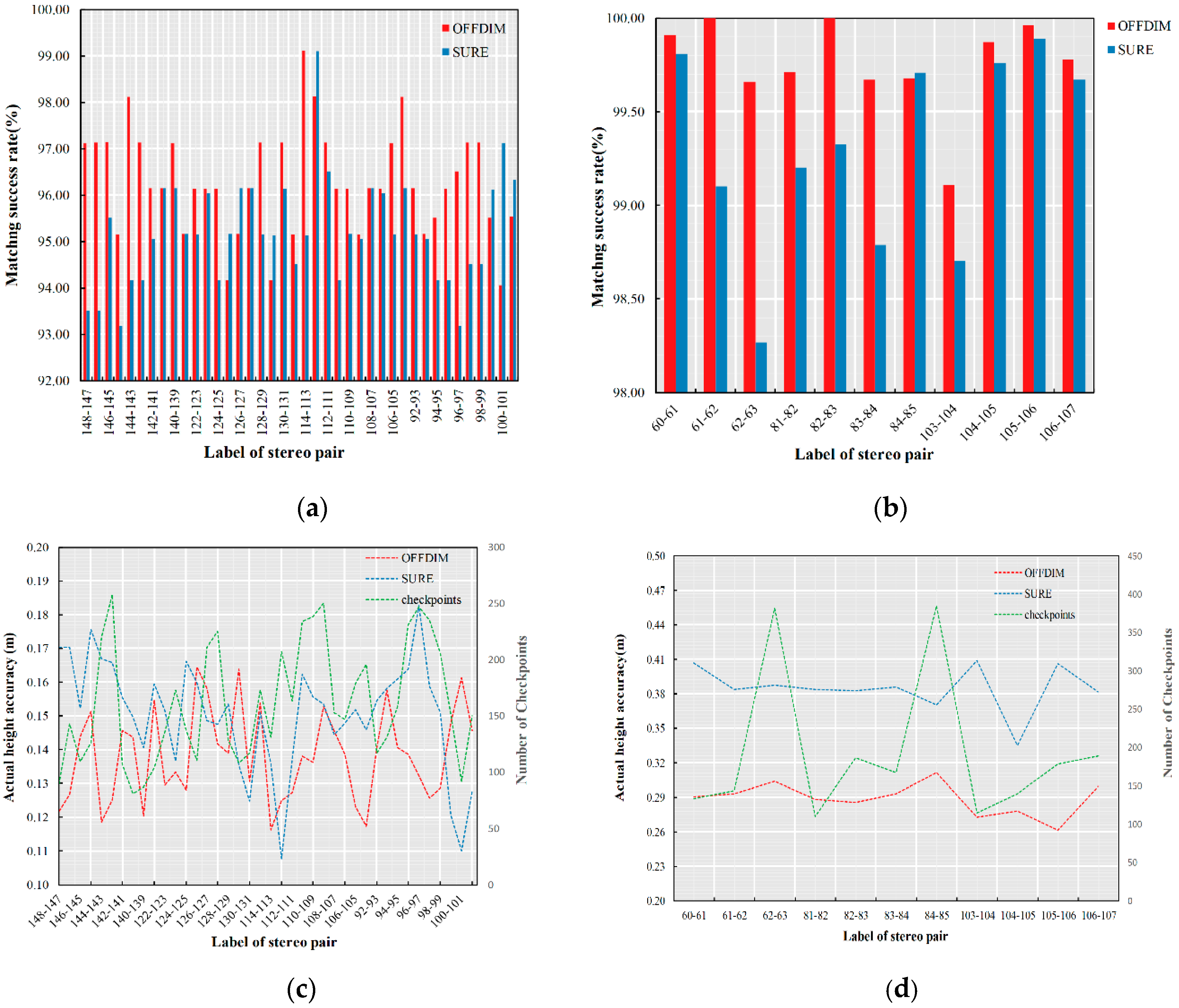
4.2. Comprehensive Comparison with SURE

The comparison software SURE is freely provided by the nFrame Company with an educational license. For two datasets, the same pre-calibrated interior camera parameters were inputted into SURE and OFFDIM, respectively. For the Vaheigen dataset, the exterior orientation elements of test images were provided by ISPRS. However, the exterior orientation elements of Beijing test images were obtained by Imagination-BBA. For two datasets, the 3D point clouds were generated on the original image resolution by SURE with the setting in dual-view.

The experiment to compare the proposed OFFDIM with SURE through visual inspection of their results was performed on both test datasets using select areas with differing textures, ranging from easy to challenging. The selected areas contained a playground, a pool with trees, continuous complex buildings, and a single building. The detailed results are presented in Figure 8.

For a more comprehensive comparison of the performances of the proposed OFFDIM and SURE, Figure 9 and

Table 2. Quantitative comparison of OFFDIM and SURE.

Dataset	Number of Images	Matching Method	Runtime (s/model)	Overall Matching Success Rate (%)	Number of Checkpoints	μ (m)
Beijing	44	OFFDIM	154.5	94.0	3077	0.1378
		SURE	402.0	93.2	3077	0.1507
Vahingen	14	OFFDIM	218.2	99.1	1529	0.2841
		SURE	327.3	98.3	1529	0.3849

present their respective matching success ratios, actual height accuracies, and computational efficiencies on the entire datasets.

It can be seen from Figure 9a,b that the matching success rates of the two methods on both test datasets are comparable, although the proposed OFFDIM’s rates of 99.1% and 94.0% MSR on the Vahingen and Beijing datasets, respectively, are a little higher than the corresponding values of 98.3% and 93.2% MSR for SURE. The matching success rate of OFFDIM for the two datasets is also comparatively more stable. When the stereo image pairs contain less difficult matching areas, such as stereo image pairs 98–99, 99–100, and 100–101 in the Beijing dataset and 84–85 in the Vahingen dataset, SURE achieves a higher matching success rate. However, when the stereo image pairs contain difficult matching areas such as tall buildings and shadowy areas, the OFFDIM is more robust.

The average actual height accuracies of the proposed OFFDIM on the Beijing and Vahingen datasets (±0.1378 and ±0.2841 m, respectively) are higher than those of SURE (±0.1507 and ±0.3849 m). It can be seen from Figure 9c,d that stereo image pairs contain 70~260 checkpoints, respectively. Here the actual height accuracy is assessed by a single stereo model. The number of checkpoints is fulfilled for the quantitative quality assessment of dense image-matching. Although the Beijing dataset has only 40 stereo image pairs and the Vahingen dataset has only 11 stereo pairs, the actual height accuracy for each stereo model is at the same level. The average height accuracy for both datasets is about ±2.5 GSD. Although these two datasets have different image resolutions and the terrain covered is totally different, the OFFDIM obtains the same matching accuracy. This demonstrates that our proposed method is stable. Additionally, the higher actual height accuracy of OFFDIM is enabled by the edge preservation of the fast-guided filter, and the penalty-based cost volume of the disparity refinement. According to Figure 9c, the smallest and largest differences between the actual height accuracies of the two methods occur for stereo image pairs 107–108 and 96–97, respectively. In the case of the stereo image pair 107–108, the main textures of the overlap area are farmland, road, and small isolated buildings. Both methods perform well on these types of textured areas. However, continuous high buildings occur in the overlap area of stereo image pair 96–97. Because tSGM (SURE) does not consider the edge information of the ground object, areas with sharp discontinuities and occlusion always fail when using the algorithm, and the disparities in such areas are thus unreliable. This is also the case for the Vahingen dataset in Figure 9d. As can be seen from Figure 9c,d, the change in the RMSE of the actual height accuracy for each stereo image pair is more stable for OFFDIM compared with SURE. This demonstrates the greater robustness of the proposed method against textural changes, and hence its feasibility for real-world applications.

The detailed computational times for the two datasets are presented in Table 2. To facilitate a computational efficiency comparison, the quality of the dense point cloud selection for SURE was set to Ultra, with the dense image-matching conducted with the original image size. The specified central processing unit (CPU) time consumption for a single stereo image pair was obtained by dividing the overall computational time for the entire dataset by the number of stereo image pairs. For a single stereo model, the mean computational time of the OFFDIM on the Beijing dataset was 154.5 s, while it was 402.0 s for SURE. However, for the Vahingen dataset, which represented an urban area, the OFFDIM and SURE computational times were 218.2 and 327.3 s, respectively. The significant computational time difference between the two methods is because SURE first analyzes all the possible overlapped stereo image pairs and conducts dense image-matching on all the possible stereo image pairs based on the selected images. When the dataset is large, the computational redundancy becomes massive. This makes the OFFDIM more efficient for handling large datasets.

4.3. Strengths and Limitations

An optical flow field-based dense image-matching algorithm is proposed in this study. The new method was successfully applied for dense 3D point cloud generation from high-resolution aerial images. The main advantage of the proposed approach is the improvement in the efficiency, completeness for stereo pair-based dense image-matching with high accuracy. Experimental results show that the average reprojection error is at the subpixel level, and actual height accuracy is about ±2.5 GSD.

According to the experimental results, OFFDIM tended to generate some unmatched pixels on the wall of a building and the roof edges as shown in Figure 8a. The reason is that we only consider the matching in a stereo pair, and the disparity of the occluded pixels are filled by the nearest valid pixels. During the 3D point cloud-generation step, some mismatched points are detected and removed, which mostly occurred in occluded areas.

5. Conclusions

Dense image-matching is a crucial step in 3D geospatial information extraction from remote-sensing images for 3D object reconstruction, DEM/digital orthophoto map (DOM) generation, and oblique photogrammetry. Although the process is well developed for close-range stereo images, it remains a significant challenge for wide-baseline aerial images owing to their large size and the presence of weak, repeated, and discontinuous textures. Conventional local cost-based algorithms may fail in the poor-texture areas, and semi-global methods encounter problems with sharp discontinuities and occlusion. Whereas the optimal global method achieves some success, it is computationally expensive. In this paper, we proposed a novel coarse-to-fine matching method, referred to as OFFDIM, that utilizes the estimation of a dense optical flow field to reduce the disparity search range, and uses a combination of the original image and a cost map to guide disparity map refinement. The proposed method involves four steps, namely, feature matching and epipolar image generation, optical flow field-based coarse-matching, cross-region-based voting and fast-guided filter-based fine-matching, and 3D point cloud generation. In the calculation of the sparse optical flow, SURF feature points and the pyramid L–K method are applied. A dense optical flow field is then estimated by a proposed TMBA method and used as the initial value for cross-region-based valid disparity range voting and fast guided filter-based fine-matching. The application of the proposed OFFDIM to two datasets with different difficult-texture areas showed that it afforded subpixel matching accuracy and actual height accuracy in excess of ±2.5 GSD. Compared with the state-of-the-art commercial software SURE, the proposed method achieved higher actual height accuracies on both test datasets (up to 26.2%) and greater matching completeness in areas with weak, repeated, and sharp discontinuous textures. The OFFDIM also reduced the total computation times for the two datasets by 61.5% and 33.3%, respectively. To the best of our knowledge, the present work represents the first use of an optical flow field to guide dense image-matching in the field of photogrammetry. The matching quality of the proposed coarse-to-fine matching strategy can be improved through the application of more effective cost volumes and global energy functions. Striking a balance between computational complexity and matching quality is another aspect worthy of further study. The algorithm of the proposed method was implemented on a CPU with parallel computing in the present study, and there is thus room for improving its efficiency through implementation on more effective platforms, and furthermore, future work will focus on improving the efficiency for large datasets.

References

1. Rothermel, M.; Haala, N. Potential of dense matching for the generation of high-quality digital elevation models. In Proceedings of the ISPRS Workshop High-Resolution Earth Imaging for Geospatial Information, Hannover, Germany, 14–17 June 2011. [Google Scholar]
2. Remondino, F.; Spera, M.G.; Nocerino, E.; Menna, F.; Nex, F. State of the art in high-density image matching. Photogramm. Rec. 2014, 29, 144–166. [Google Scholar] [CrossRef]
3. Torresani, L.; Kolmogorov, V.; Rother, C. A dual decomposition approach to feature correspondence. IEEE Trans. Pattern Anal. Mach. Intell. 2013, 35, 259–271. [Google Scholar] [CrossRef] [PubMed]
4. Scharstein, D.; Szeliski, R.; Zabih, R. A taxonomy and evaluation of dense two-frame stereo correspondence algorithms. In Proceedings of the IEEE Workshop on Stereo and Multi-Baseline Vision (SMBV), Kauai, HI, USA, 9–10 December 2001. [Google Scholar]
5. Ke, Y.; Sukthankar, R. PCA-SIFT: A more distinctive representation for local image descriptors. In Proceedings of the IEEE Conference on Computer Vision and Pattern Recognition (CVPR), Washington, DC, USA, 27 June–2 July 2004. [Google Scholar]
6. Hosni, A.; Bleyer, M.; Gelautz, M. Secrets of adaptive support weight techniques for local stereo matching. Comput. Vis. Image Understand. 2013, 117, 620–632. [Google Scholar] [CrossRef]
7. Zeglazi, O.; Rziza, M.; Amine, A.; Demonceaux, C. A hierarchical stereo matching algorithm based on adaptive support region aggregation method. Pattern Recognit. Lett. 2018, 112, 205–211. [Google Scholar] [CrossRef]
8. Wang, J.; Zickler, T. Local detection of stereo occlusion boundaries. In Proceedings of the IEEE Conference on Computer Vision and Pattern Recognition (CVPR), Long beach, CA, USA, 16–20 June 2019. [Google Scholar]
9. Tran, S.; Davis, L. 3D surface reconstruction using graph cuts with surface constraints. In Proceedings of the European Conference on Computer Vision (ECCV), Graz, Austria, 7–13 May 2006. [Google Scholar]
10. Issac, H.; Boykov, Y. Energy-based multi-model fitting and matching for 3D reconstruction. In Proceedings of the IEEE Conference on Computer Vision and Pattern Recognition (CVPR), Columbus, OH, USA, 24–27 June 2014. [Google Scholar]
11. Kim, K.R.; Kim, C.S. Adaptive smoothness constraints for efficient stereo matching using texture and edge information. In Proceedings of the IEEE International Conference on Image Processing (ICIP), Phoenix, AZ, USA, 25–28 September 2016. [Google Scholar]
12. Barron, J.T.; Adams, A.; Shih, Y.C.; Hernández, C. Fast bilateral-space stereo for synthetic defocus. In Proceedings of the IEEE Conference on Computer Vision and Pattern Recognition (CVPR), Boston, MA, USA, 7–12 June 2015. [Google Scholar]
13. Yan, T.; Gan, Y.; Xia, Z.; Zao, Q. Segment-based disparity refinement with occlusion handling for stereo matching. IEEE Trans. Image Proc. 2019, 28, 3885–3897. [Google Scholar] [CrossRef] [PubMed]
14. Tola, E.; Lepetit, V.; Fua, P. A fast local descriptor for dense matching. In Proceedings of the IEEE Conference on Computer Vision and Pattern Recognition (CVPR), Anchorage, AK, USA, 24–26 June 2008. [Google Scholar]
15. Hirschmüller, H.; Scharstein, D. Evaluation of stereo matching costs on images with radiometric differences. IEEE Trans. Pattern Anal. Mach. Intell. 2009, 31, 1582–1599. [Google Scholar] [CrossRef] [PubMed]
16. Hirschmüller, H. Stereo processing by semi-global matching and mutual information. IEEE Trans. Pattern Anal. Mach. Intell. 2008, 30, 328–341. [Google Scholar] [CrossRef] [PubMed]
17. Remondino, F.; El-Hakim, S.; Gruen, A.; Zhang, L. Turning images into 3D models. IEEE Signal. Process. Mag. 2008, 25, 55–65. [Google Scholar] [CrossRef]
18. Rothermel, M.; Wenzel, K.; Fritsch, D.; Haala, N. SURE: Photogrammetric surface reconstruction from imagery. In Proceedings of the LC3D Workshop, Berlin, Germany, 4–5 December 2012. [Google Scholar]
19. Seitz, S.M.; Curless, B.; Diebel, J.; Scharstein, D.; Szeliski, R. A comparison and evaluation of multi-view stereo reconstruction algorithms. In Proceedings of the Conference on Computer Vision and Pattern Recognition (CVPR), New York, NY, USA, 17–22 June 2006. [Google Scholar]
20. Seitz, S.M.; Dyer, C.R. Photorealistic scene reconstruction by voxel coloring. In Proceedings of the IEEE Conference on Computer Vision and Pattern Recognition (CVPR), San Juan, Puerto Rico, 17–19 June 1997. [Google Scholar]
21. Sinha, S.N.; Mordohai, P.; Pollefeys, M. Multi-view stereo via graph cuts on the dual of an adaptive tetrahedral mesh. In Proceedings of the 11th IEEE International Conference on Computer Vision (ICCV), Rio de Janeiro, Brazil, 14–20 October 2007. [Google Scholar]
22. Yoon, K.J.; Kweon, I.S. Adaptive support-weight approach for correspondence search. IEEE Trans. Pattern Anal. Mach. Intell. 2006, 28, 650–656. [Google Scholar] [CrossRef] [PubMed]
23. Bradley, D.; Boubekeur, T.; Heidrich, W. Accurate multi-view reconstruction using robust binocular stereo and surface meshing. In Proceedings of the IEEE Conference on Computer Vision and Pattern Recognition (CVPR 2008), Anchorage, AK, USA, 24–26 June 2008. [Google Scholar]
24. Geiger, A.; Roser, M.; Urtasun, R. Efficient large-scale stereo matching. In Proceedings of the Asian Conference on Computer Vision, Queenstown, New Zealand, 8–12 November 2010. [Google Scholar]
25. Habbecke, M.; Kobbelt, L. Iterative multi-view plane fitting. In Proceedings of the 11th Fall Workshop Vision, Modelling, and Visualization, Aachen, Germany, 22–24 November 2006. [Google Scholar]
26. Shan, Q.; Curless, B.; Furukawa, Y.; Hernandez, C.; Seitz, S.M. Occluding contours for multi-view stereo. In Proceedings of the IEEE International Conference on Computer Vision and Pattern Recognition (CVPR), Columbus, OH, USA, 24–27 June 2014. [Google Scholar]
27. Schönberger, J.L.; Zheng, E.; Frahm, J.M. Pixelwise view selection for unstructured multi-view stereo. In Proceedings of the European Conference on Computer Vision, Amsterdam, The Netherlands, 8–16 October 2016. [Google Scholar]
28. Furukawa, Y.; Ponce, J. Accurate, dense, and robust multi-view stereopsis. IEEE Trans. Pattern Anal. Mach. Intell. 2010, 32, 1362–1376. [Google Scholar] [CrossRef]
29. Ai, M.; Hu, Q.; Li, J. A robust photogrammetric processing method of low-altitude UAV images. Remote Sens. 2015, 7, 2302–2333. [Google Scholar] [CrossRef]
30. Shao, Z.F.; Yang, N.; Xiao, X.; Zhang, L.; Peng, Z. A multi-view dense point cloud generation algorithm based on low-altitude remote sensing images. Remote Sens. 2016, 8, 381. [Google Scholar] [CrossRef]
31. Baltsavias, E.P. Digital ortho-images—A powerful tool for the extraction of spatial-and geo-information. ISPRS J. Photogramm. Remote Sens. 1996, 51, 63–77. [Google Scholar] [CrossRef]
32. Lowe, G. SIFT-the scale invariant feature transform. Int. J. 2004, 2, 91–110. [Google Scholar]
33. Wang, Z.Z. Principles of Photogrammetry (with Remote Sensing); Publishing House of Surveying and Mapping: Beijing, China, 1990. [Google Scholar]
34. Bouguet, J.Y. Pyramidal implementation of the affine Lucas Kanade feature tracker description of the algorithm. Intel Corp. 2001, 5, 4. [Google Scholar]
35. Zabih, R.; Woodfill, J. Non-parametric local transforms for computing visual correspondence. In Proceedings of the European Conference on Computer Vision, Stockholm, Sweden, 2–6 May 1994. [Google Scholar]
36. Lee, S.; Wolberg, G.; Shin, S. Scattered data interpolation with multilevel B-splines. IEEE Trans. Visual. Comput. Graph. 1997, 3, 229–244. [Google Scholar] [CrossRef]
37. Roy, S. Stereo without epipolar lines: A maximum-flow formulation. Int. J. Comput. Vis. 1999, 24, 147–161. [Google Scholar] [CrossRef]
38. Kanade, T.; Okutomi, M. A stereo matching algorithm with an adaptive window: Theory and experiment. In Proceedings of the IEEE International Conference on Robotics and Automation, Washington DC, USA, 10–17 May 2002. [Google Scholar]
39. Min, D.B.; Lu, J.B.; Do, M.N. Joint histogram-based cost aggregation for stereo matching. IEEE Trans. Pattern Anal. Mach. Intell. 2013, 35, 2539–2545. [Google Scholar] [PubMed]
40. He, K.; Sun, J. Fast guided filter. arXiv 2015, arXiv:1505.00996. [Google Scholar]
41. Yuan, X.X. A novel method of systematic error compensation for a position and orientation system. Prog. Nat. Sci. 2008, 18, 953–963. [Google Scholar] [CrossRef]
42. Szeliski, R. Computer Vision: Algorithms and Applications; Springer: Berlin, Germany, 2010. [Google Scholar]
Figure 1. Workflow of the proposed optical flow field-based dense image-matching method (OFFDIM).
Remotesensing 11 02410 g001
Figure 2. Determination of valid disparities based on cross-region voting. (a) Determination of cross-region, and (b) cross-region voting map.
Remotesensing 11 02410 g002
Figure 3. Digital surface model automatically generated using the dense image point clouds extracted by the OFFDIM. (a) Original reference image and digital surface models generated by the (b) coarse- and (c) fine-matching of point clouds.
Remotesensing 11 02410 g003
Figure 4. Distribution of the ground control points of the Beijing dataset.
Remotesensing 11 02410 g004
Figure 5. Image coverage map of the Vahingen dataset.
Remotesensing 11 02410 g005
Figure 6. Dense image-matching results for single stereo image pairs. (a) Original image; (b) 3D point clouds; (c) dense point clouds with texture; and (d) histogram of reprojection errors.
Remotesensing 11 02410 g006
Figure 7. Dense image-matching results for difficult-to-match areas. (a) Original image patch, and (b) 3D point clouds with height map.
Remotesensing 11 02410 g007
Figure 8. Dense image-matching results for areas with different textures. Results of (a) OFFDIM and (b) SURE.
Remotesensing 11 02410 g008
Figure 9. Comparison of OFFDIM and SURE. Matching success rates on (a) Beijing (b) and Vahingen datasets; and actual height accuracies on (c) Beijing and (d) Vahingen datasets.
Remotesensing 11 02410 g009