Abstract
Acoustics is the primary means of long-range and wide-area sensing in the ocean due to the severe attenuation of electromagnetic waves in seawater. While it is known that densely packed fish groups can attenuate acoustic signals during long-range propagation in an ocean waveguide, previous experimental demonstrations have been restricted to single line transect measurements of either transmission or backscatter and have not directly investigated wide-area sensing and communication issues. Here we experimentally show with wide-area sensing over 360° in the horizontal and ranges spanning many tens of kilometers that a single large fish shoal can significantly occlude acoustic sensing over entire sectors spanning more than 30° with corresponding decreases in detection ranges by roughly an order of magnitude. Such blockages can comprise significant impediments to underwater acoustic remote sensing and surveillance of underwater vehicles, marine life and geophysical phenomena as well as underwater communication. This makes it important to understand the relevant mechanisms and accurately predict attenuation from fish in long-range underwater acoustic sensing and communication. To do so, we apply an analytical theory derived from first principles for acoustic propagation and scattering through inhomogeneities in an ocean waveguide to model propagation through fish shoals. In previous experiments, either the attenuation from fish in the shoal or the scattering cross sections of fish in the shoal were measured but not both, making it impossible to directly confirm a theoretical prediction on attenuation through the shoal. Here, both measurements have been made and they experimentally confirm the waveguide theory presented. We find experimentally and theoretically that attenuation can be significant when the sensing frequency is near the resonance frequency of the shoaling fish. Negligible attenuation was observed in previous low-frequency ocean acoustic waveguide remote sensing (OAWRS) experiments because the sensing frequency was sufficiently far from the swimbladder resonance peak of the shoaling fish or the packing densities of the fish shoals were not sufficiently high. We show that common heuristic approaches that employ free space scattering assumptions for attenuation from fish groups can lead to significant errors for applications involving long-range waveguide propagation and scattering.
1. Introduction
Acoustics is the primary means of long-range and wide-area sensing in the ocean due to the severe attenuation of electromagnetic waves in seawater. While it is known that densely packed fish groups can attenuate acoustic signals during long-range propagation in an ocean waveguide, previous experimental demonstrations have been restricted to single line transect measurements of either transmission or backscatter and have not directly investigated wide-area sensing and communication issues. Here we analyze the effects of attenuation from multiple forward scattering on instantaneous imaging of fish population densities over thousands of square kilometers with Ocean Acoustic Waveguide Remote Sensing (OAWRS) [1,2,3]. We experimentally show with wide-area sensing over 360° in the horizontal and ranges spanning many tens of kilometers that a single large fish shoal can significantly occlude acoustic sensing over entire sectors spanning more than 30° with corresponding decreases in detection ranges by roughly an order of magnitude. Such blockages can comprise significant impediments to underwater acoustic remote sensing and surveillance of underwater vehicles and geophysical phenomena as well as underwater communication. Understanding the effects of attenuation from fish is also important for conservation efforts. Climate change and overfishing have led to massive declines in marine populations, with an estimated 33 percent of marine fish stocks being harvested at unsustainable levels [4]. In order to effectively regulate fishing quotas and stabilize marine populations, it is increasingly important to develop methods for accurately surveying and monitoring fish populations over ecosystem scale areas. Low frequency (<3 kHz) acoustic sensing systems currently provide the only means of instantaneously sensing fish populations over kilometer-scale areas [2,3], however attenuation within fish shoals can reduce the strength of acoustic signals and bias population density estimates.
The potential limitations in detection range imposed by attenuation from fish makes it important to understand the relevant mechanisms and accurately predict attenuation from fish. To do so, we apply an analytical theory derived from first principles for acoustic propagation and scattering through inhomogeneities in an ocean waveguide [5] to model propagation through fish shoals. Our formulation treats multiple scatter in the forward direction. Multiple scattering in non-forward directions was found to be negligible given the packing densities and target strengths of the fish shoals we encountered based on the work of Andrews et al. [6].
The formulation used here for modeling attenuation combines waveguide scattering theory [7,8] and a differential slab marching approach introduced by Rayleigh for the mean field to derive the first two statistical moments of the acoustic field in a waveguide with inhomogeneities [5]. This formulation has been previously shown to be consistent with experimental measurements of attenuation and temporal coherence loss in the presence of internal waves for both mid-frequency signals (415 Hz) in a continental shelf environment and low-frequency signals (10-70 Hz) in a deep ocean waveguide [9,10,11].
In previous experiments, either the attenuation from fish in the shoal or the scattering cross sections of fish in the shoal were measured but not both, making it impossible to directly confirm a theoretical prediction on attenuation through the shoal [12,13]. Here, both measurements have been made and they experimentally confirm the waveguide theory presented. We study the effects of attenuation due to multiple forward scattering on sensing of herring, cod and capelin shoals in an ocean waveguide. A review of developments over past decades in wide-area underwater acoustic sensing of marine life appears in Jagannathan et al. [1]. No attenuation was measured in previously published OAWRS imagery where the acoustic sensing frequencies were off the resonance peak of the shoaling fish, including Mid-Atlantic Bight herring [3], Gulf of Maine herring [2] and Lofoten cod [14], as shown in Appendix A. Attenuation resulting in significant reductions in sound pressure level (≥10 dB) is observed in OAWRS imagery presented here of dense herring shoals collected in February 2014 near Ålesund, Norway where swimbladder resonance was near the sensing frequency.
We examine how the shadowing effects of dense fish shoals along the propagation path can be accounted for in OAWRS data to produce accurate estimates of fish areal population density using the waveguide attenuation model of Ratilal and Makris [5]. We also explore methods to predict attenuation from fish in various continental shelf environments and examine how sensing frequency can be adjusted to yield the largest detection ranges.
Attenuation from fish has also been observed in more conventional fisheries acoustics sensing methods that rely on ultrasonic sensors such as downward directed echosounders and sonars [15]. Since ultrasonic fisheries acoustic sensing employs direct paths between sensors and scatterers, modal waveguide propagation effects are not present and simple theoretical formulations derived earlier for multiple scattering in free space are valid [16,17]. These have traditionally been employed in the analysis of fisheries acoustic data where attenuation due to dense fish groups has been studied [18,19,20,21,22,23]. While free space formulations for attenuation from fish are valid for downward directed echosounders, we find that common heuristic approaches that employ free space scattering assumptions for attenuation from fish groups in long-range waveguide propagation can lead to significant errors [24,25,26].
2. Materials and Methods
Evidence of attenuation is observable in OAWRS scattering strength images of herring shoals near Ålesund, Norway. These scattering strength images are generated by beamforming, matched filtering and charting scattered returns and then correcting for source level, transmission loss and areal resolution footprint (Appendix B). Since scattering losses are not incorporated into the transmission loss, attenuation effects are visible when the scattered returns from a distant shoal diminish after an occluding shoal blocks the propagation path (Figure 1). In addition, attenuation within a single shoal is observable when the scattered returns from the shoal are strongest at the edge closest to the sensing system, with received sound pressure level decreasing with range. Ambient seafloor scattering in Figure 1 is not significantly attenuated behind the occluding shoal. This is because there is a right/left ambiguity about the horizontal line-array’s axis, so if seafloor scattering or ambient noise on one side of the ambiguity is significantly attenuated, the received signal will tend to be dominated by seafloor scattering or ambient noise from the ambiguous side. Ambiguity about the location of fish shoals in OAWRS images was resolved mainly by varying receiver ship heading [27].
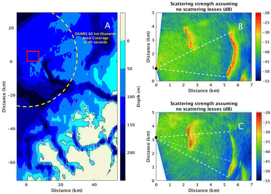
Figure 1.
Attenuation from multiple forward scattering is observable in Ocean Acoustic Waveguide Remote Sensing (OAWRS) scattering strength images of herring in Ålesund waters. Variation in bathymetry near Ålesund is shown in (A). The yellow dashed circle shows 60-km diameter OAWRS areal coverage in 40 s. The red rectangular box represents the area investigated here. OAWRS scattering strength images assuming no scattering losses are shown from 21 February 2014 at 04:50:49 (B) and 04:33:19 (C). When the propagation path from the monostatic sensing system (black dot) to the distant shoal (Easting: 5–6 km, Northing: 0–4 km) has no occluding shoal, no attenuation is observable, as shown in (B). When an occluding shoal (Easting: 2–3 km, Northing: 2–4 km) is in the propagation path, the scattered returns from the same distant shoal are attenuated, as shown in (C).
Here, we apply the formulation of Ratilal and Makris [5] to attenuation from fish shoals and demonstrate that models that ignore waveguide physics can lead to significant error (>5 dB for a given large shoal) in predicting attenuation in acoustic propagation in an ocean waveguide.
In a waveguide without scatterers, the pressure field at receiver from source at can be expressed as a sum of modes:
where is the contribution to the field by mode n. can be expressed as
where is the horizontal range, z is water depth, is the medium density at source depth and is the amplitude of acoustic mode n in the waveguide, which depends on the sound speed profile. The effects of continuous seafloor and sea surface scattering on each mode is incorporated in its complex horizontal wavenumber .
Each is normalized such that
In the formulation developed by Ratilal and Makris [5], the total mean forward field in an acoustic waveguide with scatterers can be expressed as
where each dispersion and attenuation coefficient describes the change in the horizontal wavenumber of mode n as it propagates through the scatterers. Dispersion and attenuation coefficients depend on the horizontal wavenumber , the shape of the corresponding mode , the volume density of the scatterers and the scatter function of an individual scatterer S. A general formulation for can be found in Equation (60a) of Reference [5]. Since long-range ocean sensing systems typically operate at low frequencies where the acoustic wavelength is larger than the dimensions of a fish, individual fish will be compact scatterers and the dispersion and attenuation coefficients for fish shoals can be obtained from Equations (19) and (60a) of Reference [5]:
where is the expected scatter function density of the scatterers. Since the spacing between individual fish is larger than the acoustic wavelength, the fish are incoherent scatterers and the expected scatter function density of a group of fish can be expressed as . Equations for calculating the scatter function S of an individual fish are shown in Appendix C.
The variance of the forward field can be expressed as
where is the exponential coefficient of modal field variance. A general formulation for can be found in Equation (94a) of Reference [5]. Since the scatter function of an individual fish is omnidirectional in long-range ocean sensing applications, the exponential coefficient of modal field variance for fish shoals can be obtained from Equations (19), (72) and (94a) of Reference [5]:
where the scatter function coherence volume quantifies the spatial scale over which the scatter functions of two fish are correlated. The variance of the scatter function density for incoherent scatterers can be obtained from Equations (A23) of Reference [5]:
Note that (Equation (7)) is independent of the coherence volume since the scatterers are incoherent.
The mean intensity or the second moment of the forward field is the sum of the coherent intensity and incoherent intensity:
Finally, the decrease in sound pressure level due to attenuation in the forward field from scattering can then be expressed as
As derived in Appendix D, the decrease in sound pressure level due to attenuation during two-way propagation to-and-from a uniform distribution of scatterers with mean depth and height H positioned at within resolution footprint can be similarly defined as
where is the incident field from source to target and is the field scattered from target to receiver (both defined by Equation (1)), while is the total mean intensity from source to target and is the total mean intensity from target to receiver (both defined by Equation (9)).
In the unique case where a fish shoal is uniformly distributed through the water column, we find that attenuation in a waveguide has a form approximately like that found in free space. Specifically, in this case is independent of z, so that, with Equation (3), Equation (5) can be simplified to
resulting in a total mean field equal to
If the horizontal wavenumbers of the propagating modes do not significantly deviate from the wavenumber (), we can further reduce Equation (13) using Equation (1) to yield
which has the same form as the mean field of a free space plane wave propagating through a medium with scatterers, following Rayleigh [28]. If the mean intensity is dominated by the coherent field, attenuation in a waveguide will then follow the free space form of Equation (14). We model attenuation in Ålesund waters in a case where a herring shoal uniformly covers the water column. As shown in Figure 2, the full waveguide model and the free-space-like factored approximation effectively agree, with a negligible difference between the total attenuation predicted by the two models (less than 0.5 dB).
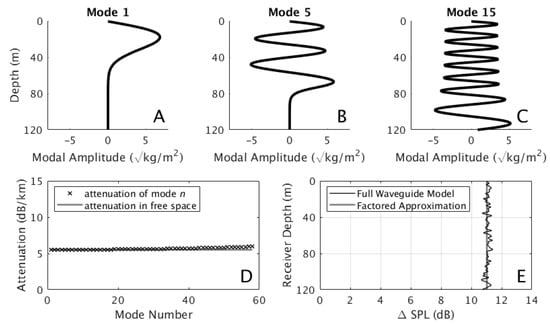
Figure 2.
When an occluding fish shoal is uniformly distributed through the water column, attenuation in a waveguide has a form similar to that in free space in that the effect of attenuation appears as a single exponential factor in received intensity, as in Equation (14). In the example shown here, attenuation of each propagating mode (A–C) differs from free space attenuation by less than 0.5 dB/km (D) and the decrease in sound pressure level due to attenuation () matches the free-space-like factored approximation within 0.5 dB at any receiver depth (E). Here, attenuation during one-way propagation is modeled for Ålesund herring with expected scatter function in a shoal uniformly distributed between the sea surface and the seafloor (0–120 m) with width 2 km and areal population density 2.5 fish/m2 estimated from echosounding data, with a source at depth 60 m with frequency 955 Hz and Ålesund sound speed profiles shown in Appendix F. Water density is modeled as 1000 kg/m2, seafloor density as 1900 kg/m2 and seafloor sound speed as 1700 m/s.
While attenuation from fish in a waveguide approximates free space attenuation when the fish uniformly cover the water column, it can differ significantly when the fish shoal is concentrated at a specific depth. We model attenuation in Ålesund waters in cases where herring are concentrated at the upper, middle and lower water column and we compare the results with a free-space-like factored approximation for attenuation of Equation (14) (Figure 3). In order to apply a free-space-like factored formulation to concentrated fish shoals, we modify the expected wavenumber change to where is the areal density of the shoal and D is the water depth. This replacement effectively "spreads" a concentrated fish shoal across the water column while retaining the total number of fish. Previous studies have modeled attenuation from fish in a waveguide using this formulation [12,29].
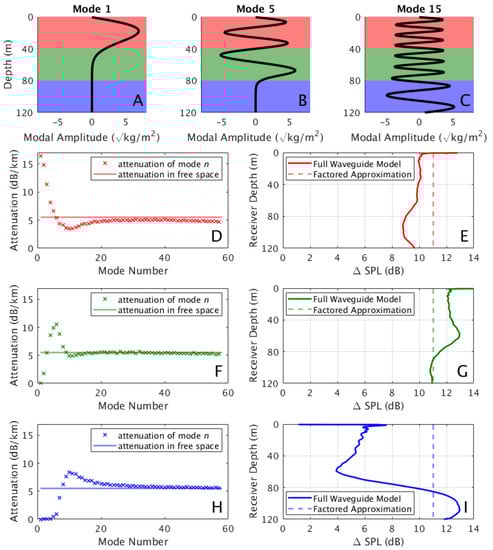
Figure 3.
When an occluding fish shoal is concentrated at a specific water depth, attenuation will be complicated by waveguide effects so that the free-space-like factored approximation of Equation (14) may not be valid. Here, attenuation during one-way propagation is modeled for Ålesund herring shoals uniformly distributed between depths 0–40 m (red), 40–80 m (green) and 80–120 m (blue). Attenuation coefficients associated with given modes and their coupling depends on the specific modal contributions at the depths where the fish group is present (A–C). Since the environment modeled here is upward refracting, the lowest order modes are most attenuated when the herring occupy the upper water column (D) but they are essentially unattenuated when the herring occupy the lower water column (H). In the case where herring are concentrated near the seafloor, a receiver in the upper water column will receive a strong signal from unattenuated lower order modes, causing the free-space-like factored approximation to overestimate the total attenuation () by more than 5 dB (I). If the herring are concentrated near the sea surface (D,E) or near the center of the water column (F,G), the free-space-like factored approximation is seen to be in error by on the order of 2 dB. Herring are modeled here with expected scatter function in a shoal with width 2 km and areal population density 2.5 fish/m2 estimated from echosounding data, with seafloor depth at 120 m, source depth at 60 m with frequency 955 Hz and Ålesund sound speed profiles shown in Appendix F. Water density is modeled as 1000 kg/m2, seafloor density as 1900 kg/m2 and seafloor sound speed as 1700 m/s.
We find that attenuation of each mode depends on the amplitude of the mode at depths where the fish are concentrated and the resulting attenuation will be strongly depth-dependent. In the upward-refracting environment modeled here, lower-order acoustic modes concentrated near the sea surface will pass through fish shoals near the seafloor with negligible attenuation and a receiver in the upper water column will measure significantly less attenuation than a receiver near the seafloor. Free-space-like factored formulations that ignore these depth-dependent modal attenuation effects can result in significant error (>5 dB for a given large shoal).
3. Results and Discussion
3.1. Consistency between Backscattered Returns and Attenuation
Here we demonstrate consistency between concurrently measured backscattering and attenuation levels from a single fish shoal using an example of attenuation from herring in Ålesund waters. In Figure 1B, there is no occluding shoal between the sensing system and a distant shoal and no attenuation is observed. In Figure 1C, the monostatic sensing system is positioned so that an occluding shoal in the propagation path attenuates the scattered returns of the distant shoal. We expect theoretical consistency between the scattering strength of the occluding shoal and the attenuation caused by the occluding shoal, where attenuation is measured as the decrease in scattered returns from the distant shoal after the occluding shoal moves into the propagation path.
The scattering strength and attenuation levels from the occluding shoal are measured using OAWRS data shown in Figure 1. The distant shoal and the occluding shoal are segmented by smoothing the scattering strength image using a circular averaging filter of radius 90 m and selecting regions with scattering strength values greater than 5 dB above the background seafloor scattering. Total two-way attenuation from the occluding shoal () is measured as the difference between the scattering strength of the distant shoal before attenuation (Figure 1B) and after attenuation (Figure 1C). Note that this measurement of assumes the areal density and vertical position of the occluding shoal and the distant shoal remain unchanged in the 17 min between the observations shown in Figure 1B,C.
When measuring scattering strength of shoals in cases where attenuation is present, care must be taken to exclude the effects of scattering loss within the shoal. We calculate the scattering strength of the occluding shoal () by selecting pixels in the shoal with scattering strength values above the 20th percentile, effectively isolating pixels at the edge of the shoal closest to the sensing system, where scattering strength is strongest and attenuation effects are negligible. This analysis is performed for all six operating frequencies used in the 2014 OAWRS experiment.
The modeled scattering strength of a shoal with mean shoal depth , shoal thickness H and neutral buoyancy depth at frequency f is calculated [30,31] from
where is the far-field scatter function of a single fish, k is the wavenumber in free space, l is the fork length of an individual fish, is the Gaussian probability density function of the fork length and z is the fish depth. Equations for modeling are shown in Appendix C. Total two-way attenuation is modeled from Equation (11) using the same five parameters used to calculate and additionally assumes the horizontal extent of the occluding shoal along the propagation path, . Note that cannot be directly determined from the scattering strength image in Figure 1 because attenuation within the occluding shoal masks the scattered returns at the far edge.
The standard deviation of the water depth along the propagation path is less than 5 m in the region where our measurements are made, which is consistent with the range-independent seafloor assumed by the current model. We verify this by using a parabolic equation model [32] to compare transmission between a flat waveguide and a varying-bathymetry waveguide using bathymetric data from the region where the experiment took place and we find the difference in transmission to be less than 1 dB.
Modeled scattering strength and attenuation values are simultaneously matched with the data using the maximum likelihood estimate of fish shoal parameters , H, , and . Since the acoustic field can be described as a circular complex Gaussian random variable (CCGR) and the time-bandwidth product of the acoustic measurements , intensity measurements in the logarithmic domain such as and can be well-approximated as Gaussian random variables with variance independent of the mean [33,34]. Since scattering strength and attenuation are dependent on many of the same parameters (, H, and ), we treat and as correlated random variables. We then estimate fish shoal parameters by maximizing the log-likelihood function assuming and are correlated Gaussian random variables with variance independent of the mean, as derived in Appendix E:
where is the variance of the measured scattering strength in dB at frequency , is the variance of the measured attenuation in dB at frequency , is the sample covariance between measured scattering strength and attenuation at frequency and is the number of frequencies where and are measured. The maximum of the log-likelihood function is determined through an exhaustive grid search across the five unknown parameters (). The ranges of these parameters are determined such that the herring shoal physically stays within the water column ( and , where D is the water depth) and the areal number density is physically realistic ( fish/m2, as determined by echosounder observations).
When fish shoal parameters are inverted by maximizing the log-likelihood function, the modeled scattering strength and attenuation values match measured values within a standard deviation, as shown in Figure 4. The inverted fish shoal depth, vertical thickness and areal density are consistent with synoptic echosounder measurements collected during the experiment (Figure A3). This consistency between scattering strength and attenuation demonstrates that the waveguide attenuation model can accurately predict attenuation levels in ocean sensing applications.
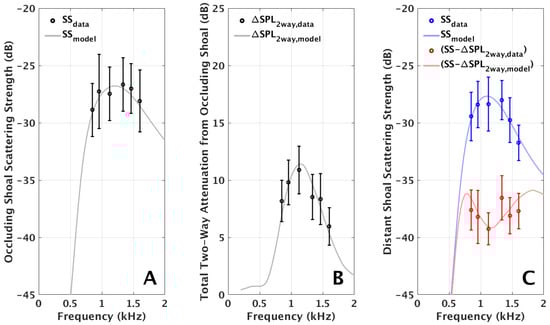
Figure 4.
Theoretical consistency is demonstrated between concurrently measured backscattering strength (A) and attenuation due to multiple forward scattering (B) from the occluding shoal shown in Figure 1. Attenuation is measured as the decrease in scattered returns from a distant shoal after the occluding shoal moves into the propagation path, that is the difference between the red and blue data in (C). Modeled scattering strength and total attenuation (grey lines in A and B, respectively) assume the same fish shoal parameters and fit the data within one standard deviation. Scattering strength and attenuation of the occluding shoal (A and B) are modeled using the following estimated parameters: mean shoal depth = 60 m, shoal thickness H = 40 m, neutral buoyancy depth = 0 m, areal number density = 2.4 fish/m2 and horizontal extent = 1.1 km. Scattering strength of the distant shoal (blue line in C) is modeled using the following estimated parameters: mean shoal depth = 85 m, shoal thickness H = 50 m, neutral buoyancy depth = 10 m and areal number density = 1.1 fish/m2.
3.2. Attenuation Prediction and Frequency Selection
Using the waveguide attenuation model, we demonstrate how sensing frequency can be adjusted to yield the largest detection range for acoustic sensing of fish shoals in various continental shelf environments. Scattering strength and attenuation are modeled for each fish species and environment and we search for the sensing frequency that maximizes scattering strength uncorrected for two-way attenuation from fish (), which in turn maximizes the detection range of the sensing system. Here is modeled using Equation (15) and is modeled using Equation (11).
We model the scattering strength uncorrected for attenuation of fish shoals in four environments: herring in the Gulf of Maine, herring in Ålesund waters, cod in Lofoten waters and capelin in Finnmark waters (Figure 5) using environmental and species-specific parameters determined from synoptic echogram data and trawl samples (Table 1). We observe a tradeoff between (1) frequencies near swimbladder resonance, where backscattering is highest but attenuation can weaken the signal and (2) frequencies off-resonance, where attenuation is negligible but backscattering is weaker. When the horizontal extent of fish along the propagation path is less than 1 km, attenuation is less of a concern and frequencies near fish swimbladder resonance are optimal. As the horizontal extent of high-density shoals in the propagation path increases, attenuation will severely limit sensing near resonance and off-resonance frequencies will become more favorable.
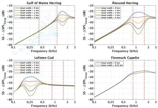
Figure 5.
The most favorable acoustic frequency for sensing in an ocean environment can be determined by maximizing the scattering strength uncorrected for two-way attenuation from fish () of a target. Here, () is modeled for fish shoals in four continental shelf environments: herring in the Gulf of Maine, herring in Ålesund waters, cod in Lofoten waters and capelin in Finnmark waters. The magnitude of attenuation depends on the width of the shoals along the propagation path between the sensing system and the target. When the shoal width along the propagation path is sufficiently small, attenuation will be negligible and the most favorable sensing frequency will be near swimbladder resonance. As the shoal width along the propagation path increases, there will be a tradeoff between frequencies near resonance where scattering strength is highest and off-resonance frequencies where attenuation is lowest. Red dotted lines designate the sensing frequency range of OAWRS experiments in each region. Physical parameters used for modeling each environment are shown in Table 1.

Table 1.
Environmental parameters used for attenuation calculations in Figure 5.
The predictions of the waveguide attenuation model shown in Figure 5 are in agreement with attenuation levels observed in previous OAWRS experiments. Significant attenuation from Ålesund herring ( > 10 dB) is predicted at the sensing frequencies used in the 2014 experiment, which is consistent with observations from that experiment. The absence of attenuation from Gulf of Maine herring in 2006 and Lofoten cod in 2014 can be explained by off-resonance sensing frequencies. Attenuation from Finnmark capelin was less than 2.5 dB even at resonance because the horizontal extent of observed capelin shoals was not large enough to produce significant attenuation (<0.25 km).
This analysis shows the waveguide attenuation model can be used to determine the conditions for significant attenuation and select sensing frequencies that maximize detection range. For example, attenuation from Ålesund herring can be avoided by choosing a sensing frequency above or below the swimbladder resonance of the fish shoals. The results of our model are specific to lower-frequency acoustic sensing, where the dimensions of a fish swimbladder are smaller than the acoustic wavelength.
3.3. Estimating Scattering Strength with Attenuation
We developed a method for accounting for attenuation in scattering strength measurements using the waveguide attenuation model. A scattering strength image uncorrected for scattering losses is generated from OAWRS data using the method described in Appendix B. In regions where scattering is dominated by fish, each scattering strength pixel can be corrected according to the following equation:
where are polar coordinates defined with respect to the monostatic sensing system, is the true scattering strength, is the scattering strength uncorrected for scattering losses and is two-way attenuation due to fish calculated from Equation (11). As shown in Equation (5), will depend on the volume density of the fish between the sensing system and the target, , which can be calculated at each pixel as a function of according [27] to
where is the areal density of the fish, H is the shoal thickness and is the target strength of an individual fish (modeled in Appendix C). As a result, each calculation of scattering strength, , depends on the scattering strength at pixels between the sensing system and the target, , so Equation (17) must be iteratively applied to pixels closest to the sensing system before correcting pixels further out.
Using this method, we modify the OAWRS scattering strength image shown in Figure 6A to include scattering losses. We designate regions where scattering is dominated by fish by smoothing the scattering strength image using a circular averaging filter of radius 90 m and selecting regions with scattering strength values greater than 5 dB above the background seafloor scattering. Corrections are made to pixels within these regions assuming the fish are uniformly distributed between depths 40 m and 80 m with neutral buoyancy depth 0 m, as determined by the parameter inversion in Equation (16).
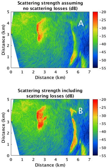
Figure 6.
The waveguide attenuation model can be used to account for scattering losses in acoustic backscattering data. Here, scattering strength images of herring shoals are shown from 04:33:19 on 21 February 2014 with (A) no scattering losses included and (B) scattering losses included. After accounting for scattering losses, the scattering strength of both the occluding shoal (Easting: 2–3 km, Northing: 2–4 km) and the distant shoal (Easting: 5–6 km, Northing: 0–4 km) are comparatively uniform in space and are not biased by the horizontal extent of fish in the propagation path. Scattering losses are calculated using the following parameters: mean shoal depth = 60 m, shoal height H = 40 m and neutral buoyancy depth = 0 m.
After modifying the scattering strength image to include scattering losses, shadowing effects caused by attenuation are no longer visible (Figure 6B). The scattering strength of the fish groups are comparatively uniform in space and are not biased by the horizontal extent of fish in the propagation path. It is important to note that scattering loss corrections cannot be made in cases where the attenuated signal is masked by ambient noise or background seafloor scattering. As a result, detection range limitations caused by attenuation from fish can only be improved by selecting a proper sensing frequency, as discussed in Section 3.2.
4. Discussion
We experimentally and theoretically demonstrate how propagation through vast and dense shoals of swimbladder-bearing fish can attenuate acoustic signals and reduce detection range for long-range sensing in the ocean as a consequence of scattering and absorption by the fish. We modeled attenuation from fish shoals in continental-shelf environments using a normal-mode based formulation derived from first principles for acoustic propagation through inhomogeneities in a waveguide. In previous experiments, either the attenuation from fish in the shoal or the scattering cross sections of fish in the shoal were measured but not both, making it impossible to directly confirm a theoretical prediction on attenuation through the shoal. Here, both measurements have been made and they experimentally confirm the waveguide theory presented. We show that common heuristic approaches that employ free space scattering assumptions for attenuation from fish groups can lead to significant error (>5 dB for a given large shoal) for applications involving long-range waveguide propagation and scattering. This same basic theory applies to fish without swimbladders, except there will be no resonance effects and attenuation is expected to be increasing with frequency as in Rayleigh-Born scattering.
5. Conclusions
We experimentally show with wide-area sensing over 360° in the horizontal and ranges spanning many tens of kilometers that a single large fish shoal can significantly occlude acoustic sensing over entire sectors spanning more than 30° with corresponding decreases in detection ranges by roughly an order of magnitude. Such blockages can comprise significant impediments to underwater acoustic remote sensing and surveillance of underwater vehicles, marine life and geophysical phenomena as well as underwater communication. We apply a rigorous formulation for modeling multiple forward scattering through inhomogeneities in an ocean waveguide to model attenuation through fish shoals in a continental shelf environment. The approach is found to accurately predict attenuation observed in Ocean Acoustic Waveguide Remote Sensing measurements over a variety of species and environments, including herring in the Georges Bank and the Nordic Seas, as well as cod and capelin in the Nordic Seas. The approach can be applied to both active and passive waveguide propagation and sensing through fish. We show that previous attenuation models that ignore waveguide physics can lead to sound pressure level predictions that are in error by at least an order of magnitude in many practical scenarios. We show that for sensing through fish shoals at frequencies near the peak swimbladder resonance of the fish, attenuation can adversely affect sensing within and beyond the shoal. In these cases, we find that the detection range of sensing systems can be maximized by choosing sensing frequencies off swimbladder resonance where attenuation is negligible. We also show how waveguide attenuation modeling can be used to more accurately estimate scattering amplitudes and fish population densities in regions where shadowing from attenuation is present.
Author Contributions
Conceptualization, N.C.M.; formal analysis, D.D., B.C., A.D.J. and N.C.M.; funding acquisition, O.R.G. and N.C.M.; investigation, D.D., A.D.J., O.R.G. and N.C.M.; methodology, D.D., B.C. and N.C.M.; project administration, O.R.G. and N.C.M.; resources, O.R.G. and N.C.M.; software, D.D., B.C., A.D.J. and N.C.M.; supervision, N.C.M.; validation, D.D., B.C. and N.C.M.; visualization, D.D., B.C., A.D.J. and N.C.M.; writing—original draft, D.D. and N.C.M.; writing—review & editing, D.D. and N.C.M.
Funding
This research was funded by Office of Naval Research grant number N00014-17-1-2197.
Conflicts of Interest
The authors declare no conflict of interest.
Appendix A. Evaluating whether Attenuation Effects are Present
Attenuation from Ålesund herring is observable when an occluding shoal moves into the propagation path to a distant shoal and the scattered returns from the distant shoal are diminished (Figure 1). The presence of attenuation is further confirmed by the steady decrease in scattering strength within the same occluding shoal as range increases (Figure A1B). We do not see evidence of attenuation from Gulf of Maine herring, Finnmark capelin and Lofoten cod, since there is not a noticeable decrease in scattering strength within a shoal as range increases (Figure A1D,F,H). These observations are consistent with the theoretical results shown in Figure 5, which predict significant attenuation from Ålesund herring and no significant attenuation from Gulf of Maine herring, Finnmark capelin and Lofoten cod at the sensing frequencies used in the OAWRS experiments.

Figure A1.
Example OAWRS scattering strength images of fish shoals assuming no scattering losses are shown from four separate continental shelf environments (A,C,E,G). Scattering strength levels along radial transects that bisect fish shoals are shown in (B,D,F,H). The positions of the radial transects are given by white lines in (A,C,E,G). We see evidence of attenuation through Ålesund herring shoals (blue line in (B)) since there is a sharp increase in scattering strength where the shoal begins (2.5 km from the source/receiver) followed by a steady decease in scattering strength caused by attenuation as range increases. After applying the attenuation correction described in Section 3.3 this effect is no longer present (red line in (B)). We do not see evidence of attenuation from Gulf of Maine herring, Finnmark capelin and Lofoten cod ((D,F,H), respectively) since there is no steady decrease in scattering strength as range increases and no attenuation correction is necessary. Sensing frequencies for the scattering strength images shown here are 955 Hz for Ålesund herring, 950 Hz for Gulf of Maine herring, 955 Hz for Lofoten cod and 1335 Hz for Finnmark capelin. Black dotted lines indicate water depth contours.

Appendix B. Measurement of Scattering Strength in OAWRS Images
Data presented here is from an OAWRS experiment conducted in 2014 to survey fish populations in the Nordic Seas via continuous monitoring with instantaneous wide-area sensing. Roughly 10,000 active transmissions were recorded at frequencies between 850 and 1600 Hz. The experiment covered multiple species in four regions in the Nordic Seas: herring in the Ålesund region were studied from 18–21 February, cod in the Lofoten region were studied on 23 February and 5–7 March, capelin in the Finnmark region were studied from 26–28 February and 1–3 March and capelin in the Tromso region were studied from 28 February through 1 March. OAWRS data was produced from active transmissions of 1 s duration linear-frequency-modulated waveforms from a vertical source array attached to the research vessel. Scattered returns from environmental features are received by a horizontal line array towed by the same research vessel with multiple nested sub-apertures. Three linear apertures of the receiver array, that is, the low-frequency (LF) aperture, the mid-frequency (MF) and the high frequency (HF) aperture, consist of 64 equally spaced hydrophones with respective inter-element spacing of 1.5 m, 0.75 m and 0.375 m. Images are generated by beamforming, matched filtering and charting scattered returns, using non-uniformly-spaced combinations of the LF, MF and HF apertures, as described in Reference [35].
The expected square magnitude of the the scattered field can be expressed as
where is the scattered field, is the reference acoustic pressure in water, is the transmitted level, is the depth-averaged two-way transmission loss to individual scatterers integrated over OAWRS imagining resolution, is the scattering strength within resolution footprint centered at horizontal location and is the decrease in sound pressure level due to two-way attenuation in the forward field from scattering [1,2,3,27]. Scattering Strength uncorrected for two-way attenuation from scattering () can then be calculated from
The is given [1] by
where
and is the Green function between the target location and the receiver location , is the horizontal target location, is the Green function between the source location and the target location , and are the sound speed and density of any point in the propagation path, respectively. A parabolic equation model [32] is used to calculate the Green functions in a range-dependent environment. The conditional expectation over the sound speed is determined by averaging five Monte-Carlo realizations, where the Green functions are calculated along the propagation path in range and depth for each realization. Each Monte-Carlo realization employs sound-speed profiles measured during the 2014 OAWRS experiment (Appendix C) every 500 m along the propagation path [36].
Appendix C. Modeling the Scatter Function of Individual Fish
The target strength of an individual fish in a shoal with mean depth and vertical thickness H is determined [1] by
where k is the wavenumber, l is the fork length of an individual fish, is the Gaussian probability density function of the fork length, z is the fish depth and S is the far-field scatter function of an individual fish, given [37] by:
where k is the wavenumber, f is the sensing frequency, is the resonant frequency of swimbladder, is the equivalent swimbladder radius and is a dimensionless damping coefficient. The equivalent swimbladder radius is determined [38] by
assuming that the swimbladder volume varies with pressure according to Boyle’s law, where is the ratio of the swimbladder volume at neutral buoyancy to the volume of the fish flesh . is the mass of a single fish empirically determined by the fork length l [27] and is the density of the fish flesh. The resonance frequency of the swimbladder is determined by
where is the ratio of the specific heats of air and is the atmospheric pressure. The correction term is a function of , the swimbladder’s eccentricity. The correction term for a prolate spheroidal swimbladder is given [39] by:
where is the ratio of the minor to major axis of a prolate spherical swimbladder given by and is the ratio of the major axis of the swimbladder to the fish fork length l [27].
The dimensionless damping coefficient in Equation (A6) is obtained from the sum of radiation damping and viscous damping :
where f is the frequency, c is the sound speed, is the viscosity of the fish flesh and is the density of fish flesh [6].
Appendix D. Modeling Two-Way Attenuation in a Waveguide Environment
In Section 2, the decrease in sound pressure level due to attenuation in the forward field in a waveguide () is derived. Here, we derive the decrease in sound pressure level due to attenuation during two-way propagation to-and-from a target in a waveguide environment ().
The two-way scattered field without attenuation from a single scatterer at with scatter function S is given by
where is the incident field from source to target and is the field scattered from target to receiver , as defined in Equation (1). Note that and assume no losses due to scatterers between and or between and . For multiple individual scatterers with scatter function S, the scattered field then becomes
Since the field is fully randomized in a ocean waveguide environment [34], the intensity can be written as
For a uniform distribution of scatterers of scatter function S with mean depth , height H and volume number density , the intensity of the scattered field without attenuation at resolution footprint can then be written as
Similarly, the mean intensity of the scattered field including attenuation can be written as
where is the total mean intensity from source to target and is the total mean intensity from target to receiver , as defined in Equation (9). Note that and take into account losses from scatterers between and and between and , respectively. Here we assume that the intensities and are uncorrelated since the field is fully randomized in a ocean waveguide environment.
The decrease in sound pressure level due to attenuation during two-way propagation can then be defined as
Appendix E. Derivation of Log-Likelihood Function
Given correlated Gaussian variables X and Y with respective means and dependent on parameter and respective variances and independent of the mean, the joint probability density of X and Y can be written as:
where
and the correlation coefficient between X and Y is defined as
where is the covariance between X and Y.
The logarithm of the probability density function will then be:
By excluding terms that are not dependent on and we are left with the log-likelihood function:
Appendix F. Sound Speed Profiles
Water-column sound speed profiles are shown in Figure A2.

Figure A2.
Profiles of water-column sound speed from XBT measurements in the Gulf of Maine (A), Ålesund waters (B), Lofoten waters (C) and Finnmark waters (D).
Figure A2.
Profiles of water-column sound speed from XBT measurements in the Gulf of Maine (A), Ålesund waters (B), Lofoten waters (C) and Finnmark waters (D).

Appendix G. Echosounder Measurements of Ålesund Herring
Synoptic echosounder measurements of Ålesund herring collected during the 2014 OAWRS experiment (Figure A3) are consistent with inverted fish shoal parameters predicted in Figure 4. Shoal volume density (fish/m3) is measured from echogram data according [27] to
where is the volume backscattering coefficient (m−1) and is the fish backscattering cross section of an individual fish at at the echosounder sensing frequency (38 kHz) in units of m2, where is the target strength at this frequency, given [40] by
where is the length of an individual herring (cm) and z is the water depth (m). Shoal areal density (fish/m2) is given by
where and delimit the depth bounds of the fish aggregations.

Figure A3.
Synoptic echosounder measurements of vertical position (A) and areal density (B) for Ålesund herring collected during the 2014 OAWRS experiment are consistent with fish shoal parameters inverted in Figure 4. White dotted lines in (A) designate the inverted vertical position of the occluding shoal (mean shoal depth = 60 m with vertical thickness H = 40 m), while the red dotted line in (B) designates the inverted areal density (2.5 fish/m2). While the echosounder measurements shown here do not directly sample the occluding shoal analyzed in Figure 4, they were recorded between 1 and 2.5 h before the OAWRS measurements of the occluding shoal and less than 10 km from its location.

References
- Jagannathan, S.; Bertsatos, I.; Symonds, D.; Chen, T.; Nia, H.; Jain, A.; Andrews, M.; Gong, Z.; Nero, R.; Ngor, L.; et al. Ocean Acoustics Waveguide Remote Sensing (OAWRS) of marine ecosystems. Mar. Ecol. Prog. Ser. 2009, 395, 137–160. [Google Scholar] [CrossRef]
- Makris, N.C.; Ratilal, P.; Jagannathan, S.; Gong, Z.; Andrews, M.; Bertsatos, I.; Godø, O.; Nero, R.; Jech, J.M. Critical population density triggers rapid formation of vast oceanic fish shoals. Science 2009, 323, 1734–1737. [Google Scholar] [CrossRef] [PubMed]
- Makris, N.C.; Ratilal, P.; Symonds, D.; Jagannathan, S.; Lee, S.; Nero, R. Fish population and behavior revealed by instantaneous continental shelf-scale imaging. Science 2006, 311, 660–663. [Google Scholar] [CrossRef] [PubMed]
- United Nations. UN Report: Nature’s Dangerous Decline ‘Unprecedented’; Species Extinction Rates ‘Accelerating’. 2019. Available online: https://www.un.org/sustainabledevelopment/blog/2019/05/nature-decline-unprecedented-report/ (accessed on 18 October 2019).
- Ratilal, P.; Makris, N.C. Mean and covariance of the forward field propagated through a stratified ocean waveguide with three-dimensional random inhomogeneities. J. Acoust. Soc. Am. 2004, 118, 3532–3558. [Google Scholar] [CrossRef]
- Andrews, M.; Gong, Z.; Ratilal, P. Effects of multiple scattering, attenuation, and dispersion in waveguide sensing of fish. J. Acoust. Soc. Am. 2011, 130, 1253–1271. [Google Scholar] [CrossRef] [PubMed]
- Ingenito, F. Scattering from an object in a stratified medium. J. Acoust. Soc. Am. 1987, 82, 2051–2059. [Google Scholar] [CrossRef]
- Makris, N.C.; Ratilal, P. A unified model for reverberation and submerged object scattering in a stratified ocean waveguide. J. Acoust. Soc. Am. 2001, 109, 909–941. [Google Scholar] [CrossRef]
- Chen, T.; Ratilal, P.; Makris, N.C. Mean and variance of the forward field propagated through three-dimensional random internal waves in a continental-shelf waveguide. J. Acoust. Soc. Am. 2005, 118, 3560–3574. [Google Scholar] [CrossRef]
- Chen, T.; Ratilal, P.; Makris, N.C. Temporal coherence after multiple forward scattering through random three-dimensional inhomogeneities in an ocean waveguide. J. Acoust. Soc. Am. 2008, 124, 2812–2822. [Google Scholar] [CrossRef]
- Gong, Z.; Chen, T.; Ratilal, P.; Makris, N.C. Temporal coherence of the acoustic field forward propagated through a continental shelf with random internal waves. J. Acoust. Soc. Am. 2013, 134, 3476–3485. [Google Scholar] [CrossRef]
- Ching, P.; Weston, D. Wideband studies of shallow-water acoustic attenuation due to fish. J. Sound. Vib. 1971, 18, 499–510. [Google Scholar] [CrossRef]
- Qiu, X.F.; Zhang, R.H.; Li, W.H.; Jin, G.L.; Zhu, B.X. Frequency-selective attenuation of sound propagation and reverberation in the Yellow Sea. J. Sound. Vib. 1999, 220, 331–342. [Google Scholar] [CrossRef]
- Makris, N.C.; Godø, O.R.; Yi, D.H.; Macauley, G.J.; Jain, A.D.; Cho, B.; Gong, Z.; Jech, J.M.; Ratilal, P. Instantaneous areal population density estimation of entire Atlantic cod and herring spawning groups and group size distribution relative to total spawning population. Fish Fish. 2019, 20, 201–213. [Google Scholar]
- Simmonds, J.; MacLennan, D.N. Fisheries Acoustics: Theory and Practice; Wiley-Blackwell: Hoboken, NJ, USA, 2008. [Google Scholar]
- Rayleigh, L. The Theory of Sound; Dover: New York, NY, USA, 1896; Volume 2, p. 196. [Google Scholar]
- Van de Hulst, H.C. Light Scattering by Small Particles; Dover: New York, NY, USA, 1957. [Google Scholar]
- Davies, I.E. Attenuation of sound by schooled anchovies. J. Acoust. Soc. Am. 1973, 54, 213–217. [Google Scholar] [CrossRef]
- Røttingen, I. On the relation between echo intensity and fish density. FiskDir. Skr. Ser. HavUnders 1976, 16, 301–314. [Google Scholar]
- Foote, K. Correcting acoustic measurements of scatter density for extinction. J. Acoust. Soc. Am. 1990, 88, 1543–1546. [Google Scholar] [CrossRef]
- Torensen, R. Absorption of acoustic energy in dense herring schools studied by the attenuation in the bottom signal. Fish. Res. 1991, 10, 317–327. [Google Scholar] [CrossRef]
- Appenzeller, A.R.; Leggett, W.C. Bias in hydroacoustic estimates of fish abundance due to acoustic shadowing: Evidence from day-night surveys of vertically migrating fish. Can. J. Fish. Aquat. Sci. 1992, 49, 2179–2189. [Google Scholar] [CrossRef]
- Zhao, X.; Ona, E. Estimation and compensation models for the shadowing effect in dense fish aggregations. ICES J. Mar. Sci. 2002, 60, 155–163. [Google Scholar] [CrossRef]
- Weston, D.; Stevens, K.; Revie, J.; Pengelly, M. Multiple frequency studies of sound transmission fluctuations in shallow water. J. Sound. Vib. 1971, 18, 487–497. [Google Scholar] [CrossRef]
- Diachok, O.; Liorzou, B.; Scalabrin, C. Estimation of the number density of fish from resonance absorptivity and echo sounder data. ICES J. Mar. Sci. 2001, 58, 137–153. [Google Scholar] [CrossRef][Green Version]
- Love, R.; Fialkowski, J.; Jagielo, T. Target strength distributions of Pacific sardine shoals: Model results at 500 Hz to 10 kHz. J. Acoust. Soc. Am. 2016, 137, 539–555. [Google Scholar]
- Gong, Z.; Andrews, M.; Jagannathan, S.; Patel, R.; Jech, J.M.; Makris, N.C.; Ratilal, P. Low-frequency target strength and abundance of shoaling Atlantic herring (Clupea harengus) in the Gulf of Maine during the Ocean Acoustic Waveguide Remote Sensing 2006 Experiment. J. Acoust. Soc. Am. 2010, 127, 104–123. [Google Scholar] [CrossRef] [PubMed]
- Rayleigh, L. On the transmission of light through an atmosphere containing small particles in suspension, and on the origin of the blue sky. Philos. Mag. 1899, 47, 375–384. [Google Scholar] [CrossRef]
- Diachok, O.; Wales, S. Concurrent inversion of geo- and bio-acoustic parameters from transmission loss measurements in the Yellow Sea. J. Acoust. Soc. Am. 2005, 128, 1965–1976. [Google Scholar] [CrossRef] [PubMed]
- Love, R. Resonant acoustic scattering by swimbladder-bearing fish. J. Acoust. Soc. Am. 1978, 64, 571–580. [Google Scholar] [CrossRef]
- Yi, D.H.; Gong, Z.; Jech, J.M.; Ratilal, P.; Makris, N.C. Instantaneous 3D continental-shelf scale imaging of oceanic fish by multi-spectral resonance sensing reveals group behavior during spawning migration. Remote Sens. 2018, 10, 108. [Google Scholar] [CrossRef]
- Collins, M. A split-step Padé solution for the parabolic equation method. J. Acoust. Soc. Am. 1993, 93, 1736–1742. [Google Scholar] [CrossRef]
- Makris, N.C. A foundation for logarithmic measures of fluctuating intensity in pattern recognition. Opt. Lett. 1995, 20, 2012–2014. [Google Scholar] [CrossRef]
- Makris, N.C. The effect of saturated transmission scintillation on ocean acoustic intensity measurements. J. Acoust. Soc. Am. 1996, 100, 769–783. [Google Scholar] [CrossRef]
- Wang, D.; Ratilal, P. Angular resolution enhancement provided by nonuniformly-spaced linear hydrophone arrays in ocean acoustic waveguide remote sensing. Remote Sens. 2017, 9, 1036. [Google Scholar] [CrossRef]
- Andrews, M.; Chen, T.; Ratilal, P. Empirical dependence of acoustic transmission scintillation statistics on bandwidth, frequency, and range in New Jersey continental shelf. J. Acoust. Soc. Am. 2009, 125, 111–124. [Google Scholar] [CrossRef] [PubMed]
- Chen, T. Mean, Variance, and Temporal Coherence of the 3d Acoustic Field Forward Propagated Through Random Inhomogeneities in Continental-Shelf and Deep Ocean Waveguides. Ph.D. Thesis, Massachusetts Institute of Technology, Cambridge, MA, USA, 2009. [Google Scholar]
- Jones, F.H.; Scholes, P. Gas secretion and resorption in the swimbladder of the cod (Gadus morhua). J. Comp. Physiol. 2018, 10, 108. [Google Scholar]
- Weston, D.E. Sound propagation in the presence of bladder fish. In Underwater Acoustics; Albers, V.M., Ed.; Plenum Press: New York, NY, USA, 1967; pp. 55–88. [Google Scholar]
- Ona, E. An expanded target-strength relationship for herring. ICES J. Mar. Sci. 2003, 60, 493–499. [Google Scholar] [CrossRef]


© 2019 by the authors. Licensee MDPI, Basel, Switzerland. This article is an open access article distributed under the terms and conditions of the Creative Commons Attribution (CC BY) license (http://creativecommons.org/licenses/by/4.0/).