Abstract
Spectral reflectance distortions caused by terrain and solar illumination seriously reduce the accuracy of mapping forest carbon density, especially in mountainous regions. Many models have been developed for mitigating or eliminating the terrain effects on the quality of remote sensing images in hilly and mountainous areas. However, these models usually use global parameters, which may lead to overcorrections for regions with poor illumination and steep slopes. In this study, we present a local parameter estimation (LPE) method based on a pixel-moving window for topographic correction (TC), which can be considered as a general optimization framework for most semiempirical TC models. We set seven kernel sizes for the presented framework, which are 15 pixels, 25 pixels, 50 pixels, 100 pixels, 250 pixels, 500 pixels, and 1000 pixels, respectively. The proposed method was then applied to four traditional TC models, Minnaert (MIN), C Correction (CC), Sun Canopy Sensor + C (SCSC) and Statistical Empirical Correction (SEC), to form four new TC models. These new models were used to estimate forest carbon density of a mountainous area in Southern China using field plot data and a Landsat 8 image. Four evaluation methods, including correlation analysis, the stability of land covers, comparison of reflectance between sunlit and shaded slopes, and accuracy assessment of forest carbon density, were employed to evaluate the contributions of moving window sizes, and assess the performance of the TC models for forest carbon density estimation. The results show that the four TC models with LPE perform much better than the traditional TC models in reducing the topographic effects and improving the estimation accuracy of forest carbon density for the study area. Among the traditional TC models, SEC performs slightly better than SCSC, CC, and MIN. Therefore, the SEC-based model with LPE, that is, LPE-SEC, gets greater R2 and smaller relative RMSE values in estimating forest carbon density than other models. Moreover, all the means of the predicted forest carbon density values fall in the confidence interval of the validation data at a significant level of 0.05. Overall, this study implies that the proposed method with LPE provides great potential to improve the performance of TC and forest carbon density estimation for the study area. It is expected that the improved TC method can be applied to other mountainous areas to improve the quality of remotely sensed images.
1. Introduction
Forests play a crucial role in the biosphere, as they mitigate carbon concentration in the atmosphere and control global warming [1,2,3]. Accurately mapping forest carbon density at different scales is of great significance for reducing greenhouse effects [4] and maintaining environmental sustainability [4,5]. Remote sensing technology has proved to be promising in estimating regional forest carbon density [6,7,8,9,10,11]. With the advantages of free downloading, wide-spatial coverage, and continuous archiving, Landsat satellite images have been widely applied in the research of forest carbon density [12,13]. However, the quality of remote sensing images is vulnerable to solar altitude, atmosphere conditions, and terrain-induced shadows, which lead to inaccuracies in spectral reflectance [14,15]. Due to terrain variation, the geometric relationships among the earth’s surface, sensors, and solar illumination are not stable, thus the solar radiation received at different locations could be significantly different [16]. The areas with the same forest type and similar slopes but different aspects may have different spectral reflectance. On the other hand, the areas with different forest types may show similar gray values due to shadows. Therefore, topographic correction (TC) is essential for improving the estimation accuracy of forest carbon density using remote sensing images, especially in China, where the mountainous areas account for 69% of the total forested land [17,18,19,20].
Since the 1980s, various TC models have been developed [21], which can be categorized into physically based models, empirical models, and semiempirical models [22]. Physically based models perform well in topographic correction as they model the full process of the interaction between solar illumination and the earth’s surface. However, these models are complex and require a large number of input parameters [23,24]. Empirical models are based on the statistical relationship between the reflectance of a location or pixel and the cosine of the relative solar incident angle [25,26]. They can be implemented without using ancillary data, but some models have parameters with no physical significance [27,28], such as statistical models. Semiempirical models adopt a digital elevation model (DEM) to represent the variation of solar illumination among different slopes [29]. To correct each spectral band, these models have to fit empirical parameters at the global level for the entire image or individually for each land cover type. Semiempirical models gain a good balance between the correction accuracy and computation efficiency, so they are widely used in the correction of terrain effects [30].
Semiempirical models can be classified into Lambertian methods and non-Lambertian methods in terms of radiation types. Lambertian models assume that the earth’s surface is a Lambertian sphere that reflects solar energy evenly in all directions. However, this assumption is inconsistent with the actual conditions and often leads to overcorrection for poor-illumination areas [20,31]. C-correction is one of the most widely used Lambertian models. Non-Lambertian methods consider the spatial optical relationship between the sun and sensor. For example, the Minnaert (MIN) model [25,32] avoids overcorrection by introducing a constant, k. However, this model is only applicable to the areas with slight terrain fluctuation, and gets low accuracy when it is applied to the areas with significant terrain fluctuations [33,34].
Some improved models have been developed to reduce the topographic effects for the regions with complex terrains, such as the sun-canopy-sensor + C (SCSC) model [30,35] and the rotation correction model [36]. Although these models can achieve sound corrections, their performance relies very much on the experimental parameters fitted by the pixel reflectance and the cosine of solar incident angles, such as the factor c for C-Correction (CC) models, factor a for rotation correction models, and constant k for MIN models. To select correction factors working well in the areas with rugged topography, the slope matching model has been proposed [25,37,38], by which different correction coefficients can be fitted according to the slope grading [39]. However, this method requires known slope grading.
Many studies have evaluated the performance of these TC models [25,38,39,40] and concluded that these models usually adopt one parameter for all pixels of one image [39], which works well only for small study areas and often lead to overcorrections for poor-illumination areas. Some stratification-based methods were proposed on the assumption that the relationship between the pixel reflectance and the cosine of relative solar incident angle is affected by different terrains, illumination [41] and land cover conditions [42]. However, these methods are too complex to be used for large and complex landscapes. Therefore, a simple and universal TC model should be developed to restore the real spectral information of remote sensing imagery in mountainous regions. For this purpose, Mo et al. [43] developed a site-specific algorithm, which has been proved to be simple, robust, and practical. However, it applies only to the rotation correction model and ignores the effects of the window sizes. Therefore, this study develops a general optimization framework that can be used to optimize traditional TC models to improve the quality of remotely sensed images in most mountainous regions. In the framework, different window sizes are used and evaluated by the correlation analysis, stability of land covers, comparison of reflectance between sunlit and shaded slopes, and accuracy assessment of forest carbon density. With the selected moving window, a local parameter estimation method was then proposed and applied to traditional TC models to form new TC models. The model with the highest correction accuracy is used to estimate the forest carbon density of the study area.
2. Data and Methods
In this study, we developed a general framework to improve the performance of TC models and forest carbon density estimation in mountainous regions. The flowchart includes three parts (Figure 1). First, field measured data, DEM and remote sensing images are preprocessed, and various spectral variables are generated. Second, a general framework based on a pixel-moving window is adopted to improve traditional TC models, in which four evaluation methods are employed to assess the contribution of window sizes for different TC models. Third, the image generated by the most accurate correction model is applied to map the forest carbon density in a mountainous region.
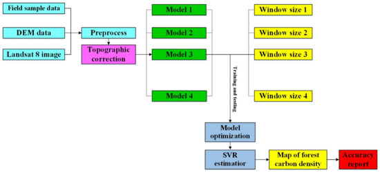
Figure 1.
The flowchart of the proposed general framework, which is developed to improve both the topographic correction and forest carbon density estimation in a mountainous region using traditional topographic correction models, Landsat 8 images and field measured data.
2.1. Study Area
The study area is located in Youxian County, eastern Hunan of China (Figure 2), which is a typical subtropical climate zone. There are steep slopes and rugged topography in this region [44], with the elevation ranging between 68 m and 1439 m and the slopes varying from 0°to 60°.
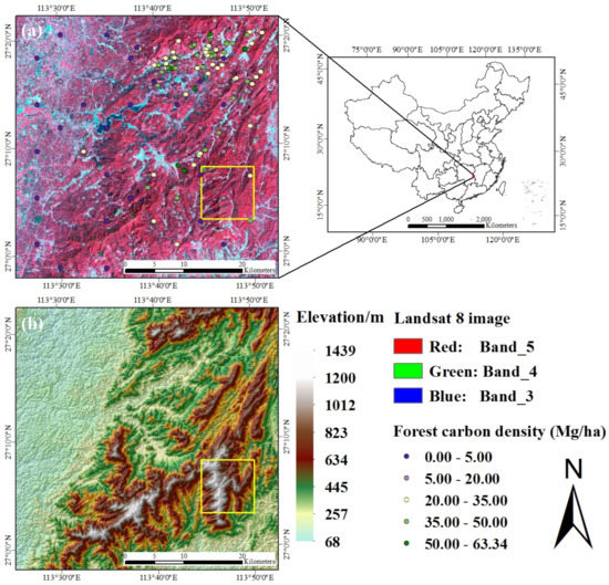
Figure 2.
(a) Location of the study area shown by a Landsat 8 false-color composite image acquired in September 2013, consisting of RGB represented by Near-Infrared, Red, and Green; (b) the topography of the study area. The area outlined by the yellow rectangle is selected for topographic correction analysis in Figure 3.
According to the data obtained by visual interpretation of the 2.5 m spatial resolution SPOT5 images, the forest coverage in this area is 86.24%, with coniferous forest 58.95%, broad-leaved forest 6.72%, bamboo 15.14%, and shrub 5.43%. Chinese fir (Cunninghamia lanceolate), Pinus massoniana Lamb, Cinnamomum camphora, Liriodendron Chinese, Cupressus funebris Endl, and Alnus cremastogyne Burk are the dominant tree species. The rest area is covered by cropland, built area, bare soil, and water. The complex illumination conditions lead to the fact that similar forest types may have different spectral reflectivity values.
2.2. Data
2.2.1. Field Measured Data
A total of 150 randomly sampled permanent plots with a size of 0.067 ha (25.82 m × 25.82 m) were collected in the summer of 2013. For the sample plots in the forested land, forest stand variables were observed by the angle gauge measurement, including the primary tree species, tree diameter at breast height, tree height, crown density, basal area at breast height and crown width. For those in the non-forested land, only the vegetation types were recorded.
To estimate the tree aboveground biomass (AGB) (trunk, branch, and leaf) by tree species in every sample plot, we measured the tree height and diameter at breast height. The AGB of each tree was obtained using the regression models by species [45]. The tree AGB was then converted to forest carbon density by the biomass-to-carbon coefficients. The sum of the forest carbon density of all tree species was the value of the sample plot. Using the models proposed in [46], we got the biomass of shrubs and herbs on the basis of their heights. Summing the biomass of each plant, we obtained the total biomass of shrubs and herbs. Dividing the total biomass by the total area, we got the per unit biomass. For the sample plots of mixed forests, the biomass values were obtained by multiplying the total biomass by the percentage of tree species. Then, a coefficient of 0.5 was adopted to convert the obtained AGB to forest carbon density. Figure 2 shows the spatial distribution of forest carbon density for the sample plots. Because the forest carbon density values of the plots were associated with uncertainties, they were considered as reference values.
2.2.2. Remote Sensing Data
In this study, we used a cloud-free (cloud cover less than 1%) Landsat 8 image acquired on September 17, 2013. It has a spatial resolution of 30 m × 30 m, similar to the size of the sample plots. Six bands of the image were selected for the analysis, which are blue (B), green (G), red (R), near-infrared (NIR), short-wave infrared1 (SWIR1) and short-wave infrared2 (SWIR2). After orthorectification, the data of the six bands were converted from digital values to top atmosphere radiance using the software of ENVI 5.3. The solar angles at the image acquisition time (solar elevation = 58.01, solar azimuth = 137.97) are typical of that of the late summer.
For enhancing the correlations between forest carbon density and spectral variables, we retrieved 200 spectral variables from the Landsat 8 image and its transformation images, including 6 original bands, 6 band inversions, 30 two-band ratios, 60 three-band ratios, 30 difference vegetation indices, 14 simple vegetation indices, 6 principal component variables, and 48 texture variables from the gray level co-occurrence matrix of the image bands [3].
2.2.3. Digital Elevation Model (DEM)
The Shuttle Radar Terrain Mission (SRTM) DEM downloaded from the USGS Earth Explore platform was selected to produce the maps of slope, aspect and illumination conditions (IC). SRTM DEM has a spatial resolution of approximate 27.6 m × 27.6 m, so it was resampled to that of the Landsat 8 image using the nearest neighborhood transformation [47]. There is no negative bias in the SRTM DEM data [48]. The study area has mountains, hills, and plains, and the mountains are mainly distributed in the northern and eastern parts.
2.3. Traditional Topographic Correction (TC) Methods
Many semiempirical methods have been developed for TC in mountainous regions, and four widely used methods were adopted in the proposed framework, which are the CC model [26,31], SCSC model [30,49], MIN model [39] and Statistical Empirical Correction (SEC) model [50,51]. The CC model takes into account the differences among the bands in diffuse radiation. The SCSC model was developed from the Sun Canopy Sensor (SCS) algorithm, and it has the advantages of both CC and SCS, which shows an excellent performance in rugged mountainous areas. The MIN correction was derived from the CC model by adding a band-specific constant k [39] and has been widely applied in the forested areas located in the mountains [31,39]. The SEC model is a statistical information-based model, which assumes that the means of the tilted and horizontal surfaces are equal. It also has been widely applied and has provided satisfactory performance [31,50,51]. According to the assumption that the terrain is horizontal [52], these models correct the rough terrain and obtain the reflectance LH(λ). The TC models are as follows:
where λ represents a specific band; LH(λ) is the corrected reflectance; LI(λ) is the observed reflectance; Z represents the solar zenith angle; c(λ) = b/a, with a and b denoting the intercept and slope of the linear regression for , respectively; IC denotes the cosine of the incidence angle; S represents the slope angle of each pixel (0 = horizontal); represents the mean value of the original reflectance; and k is a constant of Minnaert.
2.4. Topographic Correction Considering Local Parameter Estimation
For simplicity, the four TC models with local parameters are named by adding the local parameter estimation (LPE) as a prefix, such as LPE-CC, LPE-SCSC, LPE-MIN, LPE-SEC, and LPE-TC. The whole optimization process contains four steps:
Step 1: IC calculation
The IC value is calculated for each pixel by the following equation [43]:
where the solar zenith angle Z and the azimuth angle are known. Both the slope angle S and aspect angle are derived from the DEM.
Step 2: Local parameter estimation
The moving-window-based method is adopted to estimate the model parameters for each pixel by the linear regression relationship between the obtained LI(λ) and IC at the location of [i-k, i+k], [j-k, j+k] as follows [43]:
where (i, j) is the center of the moving window; k is the kernel size of the window of (2*k+1)2. a(λ)i, j is calculated for each pixel, which differs from the traditional estimation methods that use one parameter for the whole image.
Step 3: Window size determination
The efficacy of TC models is closely related to the kernel size of the moving window. Thus, we set seven kernel sizes for each of the four TC models, which are 15 pixels, 25 pixels, 50 pixels, 100 pixels, 250 pixels, 500 pixels, and 1000 pixels. The contributions of each kernel size were assessed by the correlation analysis, stability of land covers, comparison of reflectance between sunlit and shaded slopes, and accuracy assessment of forest carbon density. As one of the most popular quantitative validation methods, correlation analysis uses the correlation of the pixel reflectance against the cosine of solar incident angles, which can be measured by the reduction of the correlation coefficient in the linear regression [40,42]. Usually, the lower the correlation, the better the TC model. The stability of land cover can be measured by the relative difference of median radiance (RDMR). We classified the study area into nine land cover types and compared the RDMR for each land cover before and after TC [38,53]. Then, the area-weighted RDMR was computed for each spectral band (Equation (8)). To assess the estimation accuracy of forest carbon density, the spectral variables for the images after TC were used as the independent variables and the forest carbon density of the measured sample plots was utilized as the dependent variable [3,12,13]. Support vector regression (SVR) was then adopted for modeling, and R2 and RMSE were employed to evaluate the effects of the moving window sizes on the estimation of forest carbon density. Theoretically, the larger the value of R2 and the smaller the values of RMSE, the better the window size.
where and are the topographically corrected and uncorrected median reflectance of each band, respectively. Finally, the corrected images are obtained by Equations (1), (2), (3) and (4).
Step 4: Performance assessment
Besides the four evaluate methods mentioned above (correlation analysis, stability of land covers, comparison of reflectance between sunlit and shaded slopes, and accuracy assessment of forest carbon density), visual analysis was also conducted to quantify the performance of TC models [30,38]. Visual analysis is a subjective method because its results usually depend on the observer’s experience [30,54,55], so it should be used together with quantitative procedures.
Forest carbon density was used as the interest variable to evaluate the performances of TC models with LPE, because it is strongly related to the characteristics of forest canopies, including tree species, percentage canopy cover, the number of canopy layers and vertical structures [38,40,56]. The reflectivity of the forest canopy characteristics varies greatly over the topographic features. Theoretically, the forest carbon density estimated from the topographically corrected images should have higher accuracy than those from the original images. Thus both R2 and RMSE were applied to evaluate the contributions of the LPE-TC models on the improvement of forest carbon density estimation.
2.5. Estimation of Forest Carbon Density
In this study, the SVR algorithm was used to estimate forest carbon density. It constructs linear regression in a high-dimensional feature space and is trained based on the principle of structural risk minimization (SRM) [57,58,59,60]. The training dataset of SVR is mapped into the high-dimensional feature space using a nonlinear transformation, which is calculated by kernel functions such as the radial basis function (RBF), Gaussian, and polynomial functions [61,62]. SVR was realized by the software matlab2014a through the fitrsvm function [63].
The 150 sample plots were randomly divided into two groups: 100 for modeling and 50 for validation. In addition to RMSE and R2, other methods utilized to quantify the accuracy of forest carbon density include the residual mean, slope value of the relationship between the reference and predicted values, and the relative RMSE (RRMSE = RMSE×100/sample mean).
3. Results
3.1. Comparison of TC Models Considering LPE with Different Window Sizes
In this study, we set seven kernel sizes for each of the four TC models, which are 15 pixels, 25 pixels, 50 pixels, 100 pixels, 250 pixels, 500 pixels, and 1000 pixels. The contributions of each kernel size were assessed by correlation analysis, stability of land covers, comparison of reflectance between sunlit and shaded slopes, and accuracy assessment of forest carbon density.
3.1.1. Correlation Analysis
Table 1 shows the contributions of different kernel sizes for LPE-TC models in terms of the coefficients of determination (R2), which implies the linear relationships between IC and the reflectance of Red and NIR bands. The closer the values of R2 to zero, the less correlated the reflectance and IC, and the better the kernel sizes. In Table 1, the values of R2 change with the variation of kernel sizes, indicating that the window size has an impact on the performance of LPE-TC models. With the increase of kernel size, the R2 values increase first and then decrease. The trends are consistent for all models. When the kernel sizes increase to 100, 50, 50, 100 pixels for the models of LPE-MIN, LPE-CC, LPE-SCSC, LPE-SEC, respectively, the values of R2 reach to the minimum, respectively.

Table 1.
The determination coefficients values (R2) of the linear relationship between IC and the reflectance for the local parameter estimation-topographic correction (LPE-TC) methods with the kernel sizes ranging from 15 pixels to 1000 pixels.
3.1.2. Stability of Land Covers
The values of RDMR calculated by Equation (8) can reflect the stability of land covers. The smaller the RDMR, the better the kernel size. Table 2 compares the results of different kernel sizes of LPE-TC models based on the Red and NIR bands. With the increase of kernel size, the values of RDMR decrease first and then increase. The trends are consistent for all models. The kernel sizes between 50 and 100 pixels have relatively small values of RDMR, which implies that the kernel sizes of this range are more accurate for the LPE-TC models. These results confirm the results of correlation analysis.

Table 2.
The relative difference of median radiance (RDMR) of the improved LPE-TC models with the kernel sizes ranging from 15 pixels to 1000 pixels.
3.1.3. Comparison of Reflectance between Sunlit and Shaded Slopes
With the kernel sizes of the moving window increasing from 15 pixels to 1000 pixels, the reflectance difference of the coniferous forests between the sunlit and the shaded slopes decreases first and then increases (Table 3). The trends are consistent for all models. Similar to the stability analysis of land covers, the ideal kernel sizes are between 50 and 100 pixels. And the models of LPE-MIN, LPE-CC, LPE-SCSC, LPE-SEC with the kernel sizes of 100, 50, 50, 100 pixels, respectively, have the smallest positive values. In addition, there is a sign of overcorrection for all the models in Red band, which reduces the difference between sunlit and shaded slopes too much and leads to negative values.

Table 3.
The reflectance difference of the coniferous forests on sunlit-shaded slopes using the LPE-TC models with the kernel sizes ranging from 15 pixels to 1000 pixels.
3.1.4. Accuracy Assessment of Forest Carbon Density
The primary step of LPE-TC models is to determine the kernel size of the moving window. Table 4 shows the trends of R2 and RMSE varying with the kernel sizes. The accuracy of forest carbon density estimation changes with the kernel sizes, indicating that the window size has an impact on the estimation accuracy of forest carbon density. With the increase of kernel size, the R2 values increase first and then decrease, while the values of RMSE has an opposite trend. The trends are consistent for all models. Similar to the previous analysis, the ideal kernel sizes for forest carbon density estimation are between 50 pixels to 100 pixels. The models of LPE-MIN, LPE-CC, LPE-SCSC, LPE-SEC with the kernel sizes of 100, 50, 50, 100 pixels, respectively, have their maximum R2 and minimum RMSE. Therefore, the most suitable kernel sizes for the four TC models to improve the estimation accuracy of forest carbon density are 100, 50, 50, 100 pixels, respectively.

Table 4.
The coefficient of determination (R2) and root mean square error (RMSE) of the forest carbon density predicted by the support vector regression (SVR) algorithm using the 30 m resolution Landsat 8 image corrected by TC models considering LPE with the kernel sizes ranging from 15 pixels to 1000 pixels.
3.2. Comparison between Traditional TC Models and LPE-TC Models
After obtaining the most suitable window size, the proposed framework considering LPE was used together with four traditional TC models, which are Minnaert, C-Correction, SCSC, and SEC, to form new models for topographic correction. Similar to the determination of window sizes, the performances of these new models were assessed by visual analysis, correlation analysis, the stability of land covers, comparison of reflectance between sunlit and shaded slopes, and accuracy assessment of forest carbon density.
3.2.1. Visual Analysis
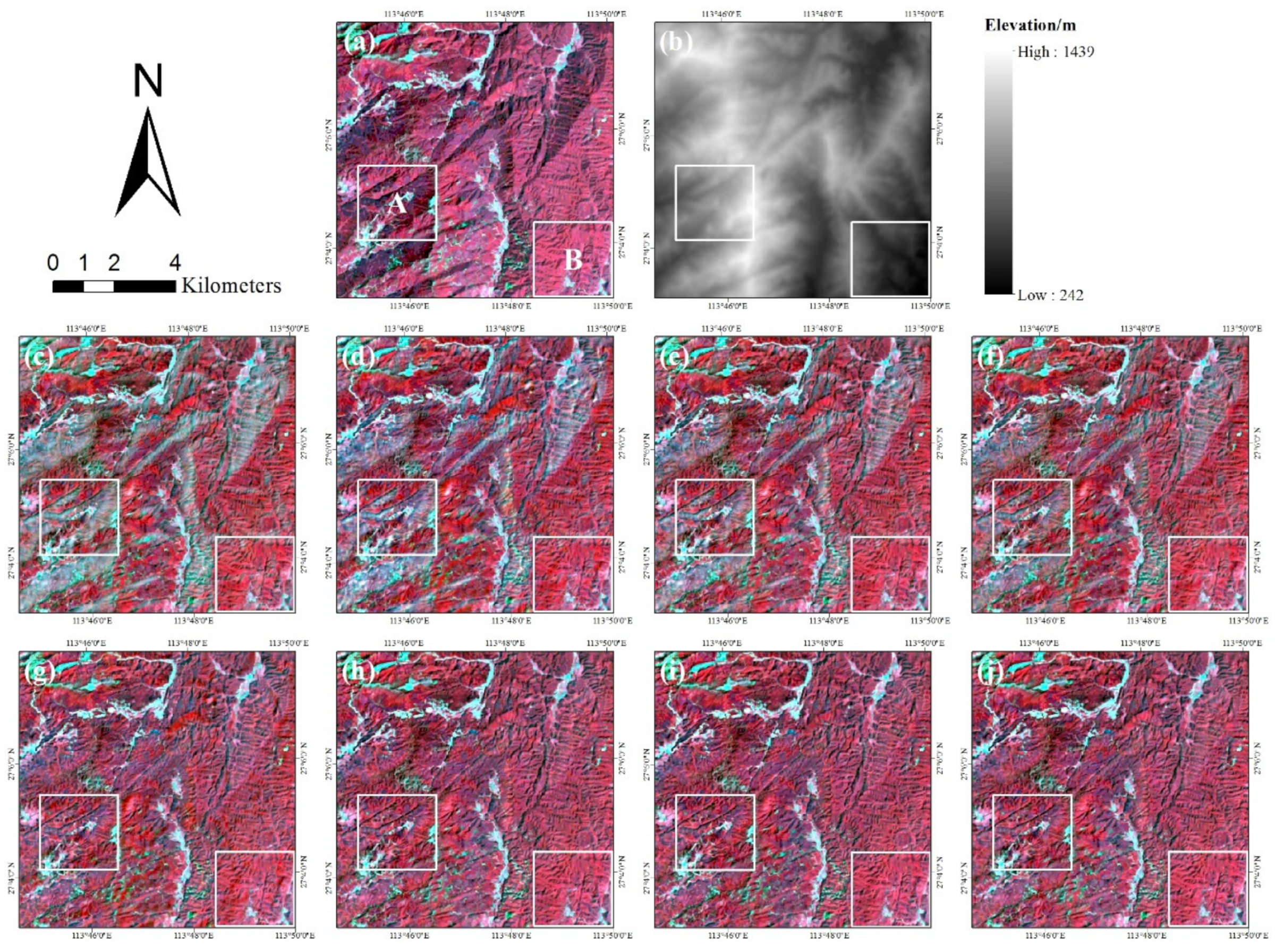
Visual analysis was adopted to compare the correction performance of the traditional TC models and LPE-TC models (Figure 3). Both the uncorrected and corrected images were compared in the false-color composites. As Figure 3a and Figure 3b show, Region B is a flat area, in which the terrain effects are very slight, so that the differences between the results are not obvious (Figure 3c to Figure 3f vs. Figure 3g to Figure 3j). Region A has strong topographic effects and shadows. All the traditional TC methods have reduced most shadow effects (Figure 3c to Figure 3f), but there are serious overcorrections in some areas, especially for the results using MIN method (Figure 3c). The LPE-TC models have removed almost all shadows in region A, including the areas without direct irradiance, and have kept most essential information (Figure 3g to Figure 3j). This indicates that the spectral heterogeneity caused by terrain has been reduced after correction, especially for the areas with the same land cover.
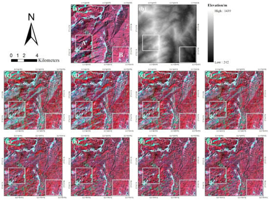
Figure 3.
The topographic correction results of the yellow rectangle region shown in Figure 2 obtained by the traditional TC methods and the TC methods considering LPE. (a) The original image, (b) DEM, and the results obtained by (c) MIN, (d) CC, (e) SCSC, (f) SEC, (g) LPE-MIN, (h) LPE-CC, (i) LPE-SCSC, and (j) LPE-SEC.
3.2.2. Correlation Analysis
As shown in Table 5, the LPE-TC models outperform the traditional TC models for each band. Moreover, among the four LPE-TC models, LPE-SEC has the smallest R2, followed by LPE-SCSC and LPE-CC, and LPE-MIN has the poorest performance. The results confirm the results of visual analysis and are consistent with the findings in other studies [26,31]. Therefore, the LPE-TC models are applicable to the images of mountainous area.

Table 5.
The determination coefficients values (R2) of the linear relationship between IC and the reflectance for the original bands and the corrected bands obtained by traditional TC methods and LPE-TC methods.
3.2.3. Stability of Land Covers
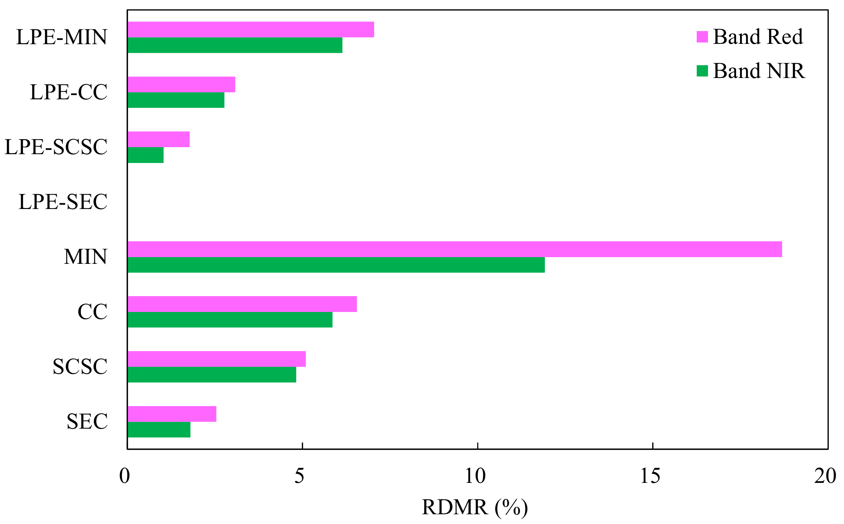
Figure 4 compares the RDMR of the traditional TC methods and the LPE-TC methods based on the Red and NIR bands. The reflectance variations are positive for all the TC methods, and smaller RDMR values mean higher correction accuracy. Compared with the traditional TC methods, the LPE-TC models have much smaller reflectance variations for both Red and NIR bands, with RDMR values smaller than 7% in most cases. As expected, the results of traditional TC models are worse, with the RDMR even close to 20% for the Red band. Overall, LPE-SEC alters the reflectance the least, with RDMR values close to zero for the two bands, followed by LPE-SCSC and SEC.
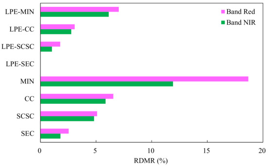
Figure 4.
The comparison of RDMR between the traditional TC models and the TC models with LPE.
3.2.4. Comparison of Reflectance between Sunlit and Shaded Slopes
In the original image, the reflectance difference of the coniferous forests between the sunlit and the shaded slopes is significant, and the NIR band even has the reflectance difference up to 33.70% (Figure 5). Compared with the original Red and NIR bands, the images corrected by traditional TC models have much smaller differences. The LPE-TC models further decrease the differences. The greatest difference reduction is achieved by LPE-SEC, then by LPE-SCSC, LPE-CC and LPE-MIN. However, all the traditional TC methods and two methods with LPE (LPE-CC and LPE-MIN) reduce this difference too much and result in negative values in the Red band, which is a sign of overcorrection. The results of the LPE-SEC model have the smallest positive value, implying that the LPE-SEC method is better than other methods. This finding is consistent with that of the stability analysis of land cover.
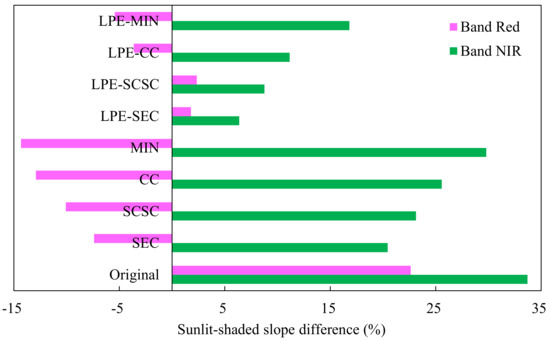
Figure 5.
The reflectance difference of the coniferous forests on sunlit-shaded slopes (wm−2sr−1μm−1) between the traditional TC models and the LPE-TC models. The smaller the difference, the better the correction result.
3.2.5. Accuracy Assessment of Forest Carbon Density
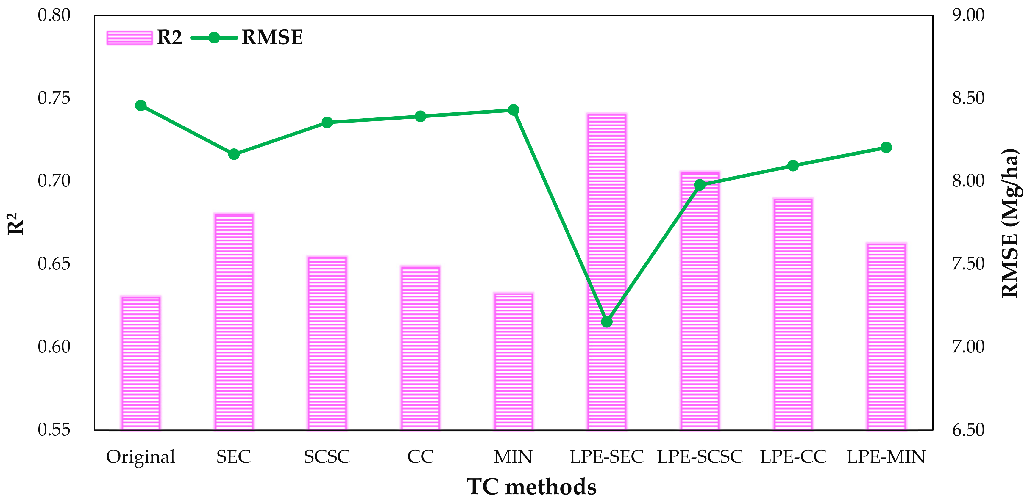
In order to evaluate the contribution of LPE on the estimation of forest carbon density, we compared the forest carbon density predicted by SVR using the original image, the images corrected by traditional TC models and the images corrected by LPE-TC models. Figure 6 shows that the results of the original image have the smallest R2 value and largest RMSE value. Compared with the original image, the results of corrected images have larger R2 and smaller RMSE. The LPE-TC models further increase R2 and reduce RMSE. Among the LPE-TC models, LPE-SEC has the highest accuracy with the largest R2 and the smallest RMSE, followed by LPE-SCSC, LPE-CC, and LPE-MIN. This indicates that all TC models can improve the estimation accuracy of forest carbon density, but the LPE-TC models outperform traditional TC models, and the LPE-SEC model leads to the highest estimation accuracy of forest carbon density.

Figure 6.
The R2, and root mean square error (RMSE) of the forest carbon density predicted by SVR using the original image, the images corrected by traditional TC models and the images corrected by LPE-TC models.
3.3. Estimation of Forest Carbon Density
3.3.1. Statistics of Sample Plots
The statistical results of forest carbon density are listed in Table 6, which were calculated from the sample plots of the study area. All the plots have a sample mean of 28.42 Mg/ha, with standard deviation and coefficient of variation being 13.46 Mg/ha and 47.37%, respectively. The modeling dataset has a slightly smaller mean and larger standard deviation and coefficient of variation than the validation dataset and whole dataset. At the significant level of 0.05, there are no significant differences among the mean values of three datasets. The confidence intervals are (26.27, 30.57), (24.75, 30.07), (26.71, 34.07) (Mg/ha) for the whole dataset, modeling dataset and validation dataset, respectively.

Table 6.
Statistical results of the forest carbon density calculated from the sample plots. SD and CV indicate the standard deviation and coefficient of variation, respectively.
3.3.2. Correlation Analysis
The correlation coefficients between the spectral variables and the measured forest carbon density range from −0.508 to 0.617, −0.533 to 0.635, and −0.551 to 0.650 for the original image, the image corrected by SEC and the image corrected by LPE-SEC, respectively. For these three kinds of images, there are 48, 54, and 65 spectral variables significantly correlated with the measured forest carbon density at a significant level of 0.05, respectively. For simplicity, Table 7 only presents the five most correlated variables. The variable NIR/SWIR2 from all the three kinds of images is the most correlated with the plot forest carbon density. Interestingly, almost all listed spectral variables are relevant to NIR and Red bands, and their band ratios reduce the slope effect in the rugged mountainous areas.

Table 7.
Correlation coefficients between the measured forest carbon density and spectral variables from the original images and the images corrected by the traditional SEC model and the LPE-SEC model, respectively.
3.3.3. Accuracy Assessment
We estimated the forest carbon density by combining the sample plot data with the original image, the image corrected by SEC and the image corrected by LPE-SEC, separately. The estimation accuracies are assessed based on the validation data (Table 8). At the significant level of 0.05, all the means of the predicted forest carbon density values fall within the confidence intervals of the validation dataset. However, all the mean values are slightly over-estimated, especially the results from the original image.

Table 8.
Estimation accuracy of the forest carbon density by combining the sample plot data with the original image and the images corrected by the traditional SEC and LPE-SEC, respectively. R2: determination coefficient. RMSE: root mean square error. At the significance level of 0.05, the confidence interval of the validation data is (26.71, 34.07) (Mg/ha).
Moreover, the coefficient of determination (R2) between the reference value and the estimated value increases significantly. For the R2 value resulted from the LPE-SEC corrected image, more than 74% changes of the reference values can be accounted for by the predicted values. The RMSE and RRMSE from all the images are similar, but they are smaller for the TC corrected images, especially the image corrected by LPE-SEC. However, there are statistically significant differences for RMSE and RRMSE between the original image and the image corrected by the traditional TC model. The LPE-SEC method performs significantly better than traditional methods in improving the estimation precision of the forest carbon density in mountainous regions.
3.3.4. Spatial Analysis
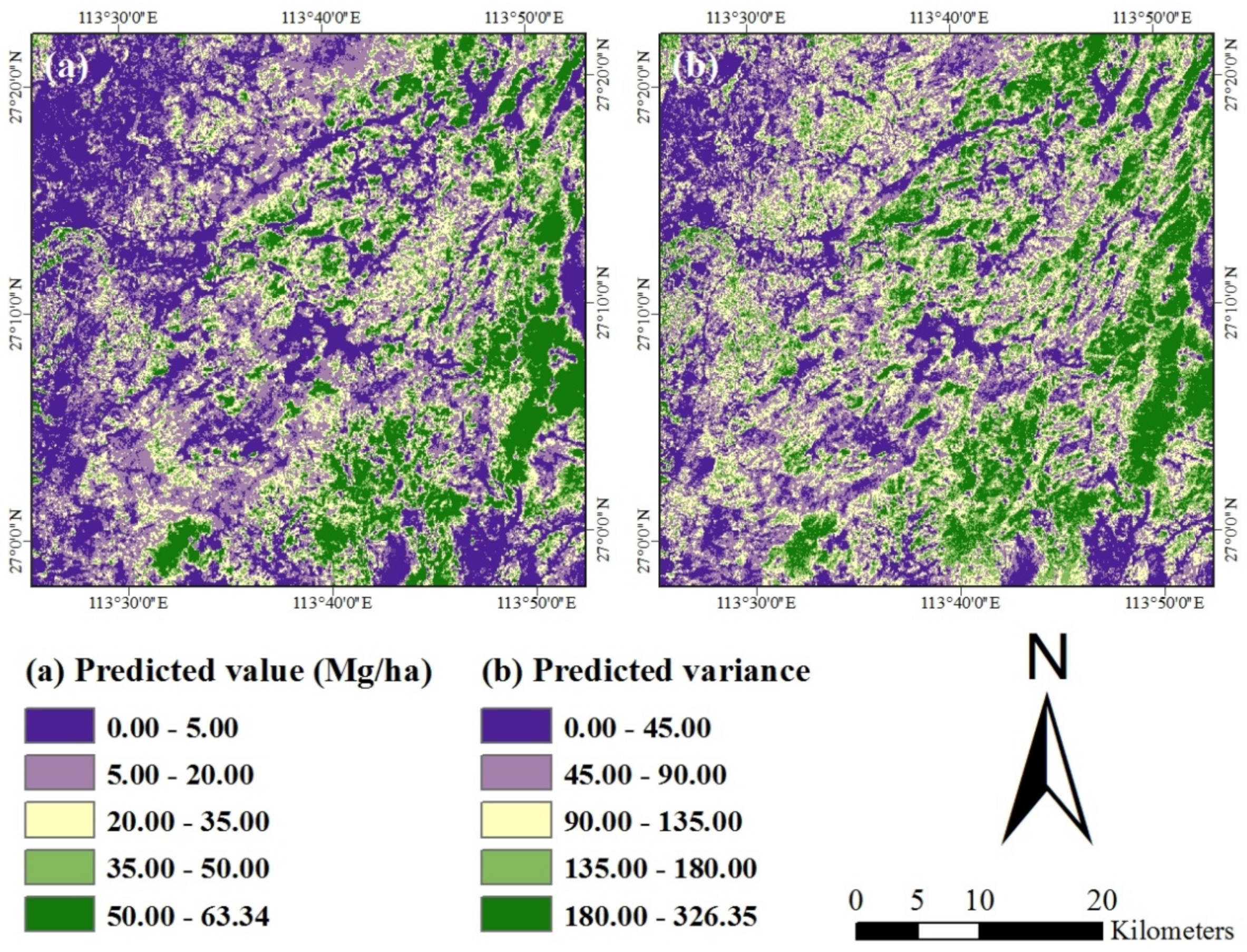
By combining the sample plot data with the LPE-SEC corrected image, we got the maps of forest carbon density and its variance using SVR (Figure 7). The spatial distribution of the predicted forest carbon density values is similar to those of the sample plots and the Landsat 8 image. The high values of forest carbon density concentrate in the east-central, southeast, and northeast areas, where the corresponding variances are also significant.
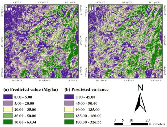
Figure 7.
The maps of (a) forest carbon density and (b) its variances predicted by support vector regression (SVR) using the sample plot data combined with the LPE-SEC corrected image.
4. Discussion
In this study, a general framework considering local parameter estimation (LPE) based on a pixel-moving window was proposed for topographic correction. The comparison between the four traditional TC models and those considering LPE indicates that the proposed framework is simple and effective, and could be used as a general optimization framework for most current semiempirical TC models. The results also show that the proposed framework can significantly improve the performance of traditional TC models, thus increase the estimation accuracy of forest carbon density in the mountainous area.
4.1. Comparison of TC Models Considering LPE with Different Kernel Sizes
In this study, the optimal kernel size of the moving window was finally determined by correlation analysis, stability of land covers, comparison of reflectance between sunlit and shaded slopes, and accuracy assessment of forest carbon density. Results show that the optimal kernel sizes vary from 50 pixels to 100 pixels over different TC models, which implies different window sizes have different effects on the accuracy of forest carbon density estimation. Noting the estimation of forest carbon density is also affected by factors such as forest type, site quality, sample data and image quality [3]. For simplicity, these factors were assumed to be the same in our study. Thus the window size should be the only factor affecting the estimation accuracy of forest carbon density. Although such assumption makes it easy to analyze the contributions of window sizes, some uncertainties may result. If the framework is applied to map forest carbon density of complicated rainforests, these factors should be taken into account to optimize the procedure of window size selection [32,38,64]. In addition, the results may be further improved by matching the topographic relief with the sizes of moving windows. Further efforts should be made to eliminate the side effects of various moving windows.
4.2. Comparison between Traditional TC Models and TC Models Considering LPE
According to the correlation analysis, the LPE-TC models perform better than the traditional TC models in reducing the dependence of spectral reflectance on IC, which is consistent with the results of visual analysis. Other assessments also illustrate the superiority of the framework considering LPE. Robustness and stability tests show that the framework considering LPE can improve the quality of remote sensing images by reducing the topographic effects.
Among the LPE-TC models, LPE-SEC performs better than the other methods in reducing the topographic effect, followed by LPE-CC, LPE-SCSC, and LPE-MIN. This is because the study area is dominated by coniferous forests that have homogeneous canopy structures. The LPE-SEC model, as a statistical method based on mean approximation, can generate more accurate results than the other models [28]. The LPE-MIN method has the poorest correction accuracy, which is consistent with the findings of [28] that claimed larger solar elevation angles might bring better performances. However, some researchers suggested that the poor results from the solar elevation angle smaller than 25° [28] should be attributed to the different image acquisition times (such as in August and December). For example, Sola et al. [32] obtained poor results using the image from December with a solar elevation angle of 21°.
In this study, all the LPE-TC models have higher estimation accuracy of forest carbon density than traditional TC models, which confirms the great potential of using LPE to improve the forest carbon density estimation in mountainous regions. The reason may be that the local parameter estimation not only successfully reduces the influence of local terrain, but also captures the detailed information of the pixels and suppresses the image noise effectively. Compared with the methods mentioned in [39,41,42], the proposed method is more generalized and can be integrated with most semiempirical TC models, which leads to a general framework for optimizing topographic correction of images. Moreover, this framework can be used for the estimation of forest carbon density in large scale and complex landscapes, but it requires intensive computation. With the development of computer technology, the limitation will become less serious.
4.3. Estimation of Forest Carbon Density
The images corrected by LPE-SEC and SEC were applied to estimate the forest carbon density using the SVR [65,66,67] algorithm and led to the relative RMSE values of 23.50% and 26.54%, respectively. The estimation accuracy of the LPE-SEC corrected image is much higher than that of the original image and those of [3,68] at the same plot scale, due to the reduction of terrain effects and consideration of local parameter estimation. It implies that the framework considering LPE provides the potential of increasing the estimation accuracy of forest carbon density in the mountainous area.
Although SVR has certain advantages over traditional regression methods, the selection of kernel functions and the determination of parameters may influence the accuracy of the prediction model. This study focuses on proposing a universal optimization framework adaptive to traditional TC methods in mountainous regions, thus which estimation method should be used to estimate forest carbon density would not influence the conclusions of this research [3]. However, the improvement and optimization of SVR need study, especially the kernel function selection and parameter determination.
4.4. Computation Load for the Framework Considering LPE
In the proposed framework, each step involved in the local parameter estimation was carried out for each pixel, so the computation load is huge if there are many pixels in an image. In this study, the computation was done by a computer with an Intel Core i7-3470 CPU (3.20 GHz), 12G RAM, and 64-bit Windows 7 operating system and cost 53.188 s per band for the image with a size of 1000 pixels × 1000 pixels. Parallel computing may greatly reduce the computation load. Also, a more adaptive local parameter estimation method could improve the computation efficiency.
5. Conclusions
In this study, a methodology considering LPE was proposed to improve topography correction and forest carbon density estimation in the mountainous regions using traditional TC models, Landsat 8 images and field measured data. This methodology was considered as a general optimization framework that can be jointly used with most semiempirical TC models for the topographic correction of most mountainous regions. The method can correct the reflectance distortions caused by local topographic effects. As expected, the experiment results suggest that all the TC models considering LPE perform significantly better than the traditional TC models in reducing topographic effects and improving the estimation accuracy of forest carbon density for the mountainous area. Among the traditional TC models, SEC performs slightly better than SCSC, CC, and MIN. Therefore, LPE-SEC results in larger R2 and smaller relative RMSE than the other LPE-TC models and all traditional TC models for forest carbon density estimation. Moreover, the estimation accuracies of forest carbon density using the image corrected by both the traditional and improved TC methods are higher than that from the original image. In addition, all the means of the predicted forest carbon density values fall in the confidence interval of the validation data at a significant level of 0.05. Overall, this study implies that the proposed methodology considering LPE has great potential in improving topographic correction and forest carbon density estimation for mountainous areas. However, future research is necessary to confirm the robustness of this framework.
Author Contributions
E.Y. and D.M. designed the study. E.Y. conducted the experiments and wrote the draft. D.M. carried out the optimization of the framework. E.Y. and D.M. collected the field survey data and completed the calculations of forest carbon density. Y.Z. and H.L. provided comments. E.Y. and G.W. revised the manuscript.
Funding
This paper was supported by National Natural Science Foundation of China (31901311, 31470643): Study on the optimization of topographic correction for estimating forest carbon density in mountainous regions using remote sensing technology & theory and technology research of ground truth samples design based on segmented objects from satellite imagery; China Postdoctoral Science Foundation (2017M620362): Model research of topographic correction for monitoring forest types in mountainous regions using remote sensing technologies; Hunan Provincial Natural Science Foundation of China (2018JJ3871): Effect analysis of topographic correction on the estimation accuracy of forest carbon density in mountain area.
Acknowledgments
The authors are grateful to Huang-Feng-Qiao forest farm of Youxian County for technical support on field data collection.
Conflicts of Interest
The authors declare no conflict of interest.
References
- Schimel, D.; House, J.; Hibbard, K.; Bousquet, P.; Ciais, P.; Peylin, P.; Braswell, B.H.; Apps, M.J.; Baker, D.; Bondeau, A.; et al. Recent patterns and mechanisms of carbon exchange by terrestrial ecosystems. Nature 2001, 414, 169–172. [Google Scholar] [CrossRef] [PubMed]
- Yan, E.; Lin, H.; Wang, G.; Sun, H. Improvement of forest carbon estimation by integration of regression models and spectral unmixing of Landsat data. IEEE Geosci. Remote Sens. Lett. 2015, 12, 2003–2007. [Google Scholar]
- Yan, E.; Lin, H.; Wang, G.; Sun, H. Multi-resolution mapping and accuracy assessment of forest carbon density by combining image and plot data from a nested and clustering sampling design. Remote Sens. 2016, 8, 571. [Google Scholar] [CrossRef]
- Nabuurs, G.; Putten, B.; Knippers, T.; Mohren, G. Comparison of uncertainties in carbon sequestration estimates for a tropical and a temperate forest. For. Ecol. Manag. 2008, 256, 237–245. [Google Scholar] [CrossRef]
- Luo, K.S. Spatial pattern of forest carbon storage in the vertical and horizontal directions based on HJ-CCD remote sensing imagery. Remote Sens. 2019, 11, 788. [Google Scholar] [CrossRef]
- Kim, S.; Lee, W.; Kwak, D.; Biging, G.; Gong, P.; Lee, J.; Cho, H. Forest cover classification by optimal segmentation of high-resolution satellite imagery. Sensors 2011, 11, 1943–1958. [Google Scholar] [CrossRef]
- Zhang, Z.; Kazakova, A.; Moskal, L.; Styers, D. Object-based tree species classification in urban ecosystems using LiDAR and hyperspectral data. Forests 2016, 7, 122. [Google Scholar] [CrossRef]
- Tian, S.; Zhang, X.; Tian, J.; Sun, Q. Random forest classification of wetland land covers from multi-sensor data in the arid region of Xinjiang, China. Remote Sens. 2017, 8, 954. [Google Scholar] [CrossRef]
- Hughes, R.; Asner, G.; Baldwin, J.; Mascaro, J.; Bufil, L.; Knapp, D. Estimating aboveground carbon density across forest landscapes of Hawaii: Combining FIA plot-derived estimates and airborne LiDAR. For. Ecol. Manag. 2018, 424, 323–337. [Google Scholar] [CrossRef]
- Berninger, A.; Lohberger, S.; Stängel, M.; Siegert, F. SAR-based estimation of above-ground biomass and its changes in tropical forests of Kalimantan using L- and C-band. Remote Sens. 2018, 10, 831. [Google Scholar] [CrossRef]
- Hirata, Y.; Furuya, N.; Saito, H.; Pak, C.; Leng, C.; Sokh, H.; Ma, V.; Kajisa, T.; Ota, T.; Mizoue, N. Object-based mapping of aboveground biomass in tropical forests using LiDAR and very-high-spatial-resolution satellite data. Remote Sens. 2018, 10, 438. [Google Scholar] [CrossRef]
- Li, Y.; Han, N.; Li, X.; Du, H.; Mao, F.; Cui, L.; Liu, T.; Xing, L. Spatiotemporal estimation of bamboo forest aboveground carbon storage based on Landsat data in Zhejiang, China. Remote Sens. 2018, 10, 898. [Google Scholar] [CrossRef]
- Zhu, J.; Huang, Z.; Hua, S.; Wang, G. Mapping forest ecosystem biomass density for Xiangjiang River Basin by combining plot and remote sensing data and comparing spatial extrapolation methods. Remote Sens. 2017, 9, 241. [Google Scholar] [CrossRef]
- Fan, W.; Li, J.; Liu, Q.; Zhang, Q.; Yin, G.; Li, A.; Zeng, Y.; Xu, B.; Xu, X.; Zhou, G.; et al. Topographic correction of forest image data based on the canopy reflectance model for sloping terrains in multiple forward mode. Remote Sens. 2018, 10, 717. [Google Scholar] [CrossRef]
- Lars, E.S. Topographic effects in Geoid determinations. Geosciences 2018, 8, 143. [Google Scholar] [CrossRef]
- Melnikova, M.; Awaya, Y.; Saitoh, T.M.; Muraoka, H.; Sasai, T. Estimation of leaf area index in a mountain forest of central Japan with a 30-m spatial resolution based on Landsat operational Land imager imagery: An application of a simple model for seasonal monitoring. Remote Sens. 2018, 10, 179. [Google Scholar] [CrossRef]
- Zhang, Z.; He, J.; Liu, D.; Wang, X.; Jiang, H. An improved physical model to correct topographic effects in remotely sensed imagery. Spectrosc. Spectr. Anal. 2010, 30, 1839–1842. [Google Scholar]
- Duan, S.; Shi, K.; Lu, Z. Research on topographic correction of remotely sensed image in rugged terrain areas based on SRTM3. Sci. Technol. Eng. 2012, 12, 8147–8153. [Google Scholar]
- Wang, S.; Li, X.; Zhang, Q.; Chen, X.; Ye, W. Analysis on the applicability of the topographic correction models for Landsat images. J. Huazhong Norm. Univ. 2013, 47, 571–577. [Google Scholar]
- Li, A.; Wang, Q.; Bian, J.; Lei, G. An improved physics-based model for topographic correction of Landsat TM images. Remote Sens. 2015, 7, 6296–6319. [Google Scholar] [CrossRef]
- Ediriweera, S.; Pathirana, S.; Danaher, T.; Nichols, D.; Moffiet, T. Evaluation of different topographic corrections for Landsat TM data by Prediction of Foliage Projective Cover (FPC) in topographically complex landscapes. Remote Sens. 2013, 5, 6767–6789. [Google Scholar] [CrossRef]
- Balthazar, V.; Vanacker, V.; Lambin, E. Evaluation and parameterization of ATCOR3 topographic correction method for forest cover mapping in mountain areas. Int. J. Appl. Earth Obs. Geoinf. 2012, 18, 436–450. [Google Scholar] [CrossRef]
- Zhang, W.; Gao, Y. Topographic correction algorithm for remotely sensed data accounting for indirect irradiance. Int. J. Remote Sens. 2011, 32, 1807–1824. [Google Scholar] [CrossRef]
- Couturier, S.; Gastellu-Etchegorry, J.; Martin, E.; Patiño, P. Building a forward-mode three-dimensional reflectance model for topographic normalization of high-resolution (1–5 m) imagery: Validation phase in a forested environment. IEEE Trans. Geosci. Remote Sens. 2013, 51, 3910–3921. [Google Scholar] [CrossRef]
- Richter, R.; Kellenberger, T.; Kaufmann, H. Comparison of topographic correction methods. Remote Sens. 2009, 1, 184–196. [Google Scholar] [CrossRef]
- Gao, Y.; Zhang, W. A simple empirical topographic correction method for ETM+ imagery. Int. J. Remote Sens. 2009, 30, 2259–2275. [Google Scholar] [CrossRef]
- Blesius, L.; Weirich, F. The use of the Minnaert correction for land-cover classification in mountainous terrain. Int. J. Remote Sens. 2005, 26, 3831–3851. [Google Scholar] [CrossRef]
- Li, H.; Xu, L.; Shen, H.; Zhang, L. A general variational framework considering cast shadows for the topographic correction of remote sensing imagery. ISPRS J. Photogramm. Remote Sens. 2016, 117, 161–171. [Google Scholar] [CrossRef]
- Reese, H.; Olsson, H. C-correction of optical satellite data over alpine vegetation areas: A comparison of sampling strategies for determining the empirical c-parameter. Remote Sens. Environ. 2011, 115, 1387–1400. [Google Scholar] [CrossRef]
- Soenen, S.; Peddle, D.; Coburn, C. SCS+C: A modified sun-canopy-sensor topographic correction in forested terrain. IEEE Trans. Geosci. Remote Sens. 2005, 43, 2148–2159. [Google Scholar] [CrossRef]
- Hantson, S.; Chuvieco, E. Evaluation of different topographic correction methods for Landsat imagery. Int. J. Appl. Earth Obs. Geoinf. 2011, 13, 691–700. [Google Scholar] [CrossRef]
- Sola, I.; María, G.; Jesús, Á. The added value of stratified topographic correction of multispectral images. Remote Sens. 2016, 8, 131. [Google Scholar] [CrossRef]
- Huang, B.; Xu, L. Applied research of Topographic correction based on the improved Minnaert model. Remote Sens. Technol. Appl. 2013, 27, 183–189. (In Chinese) [Google Scholar]
- Uday, P.; Asamaporn, S.; Dario, S.; Sukan, P.; Kumron, L.; Amnat, C. Topographic correction of Landsat TM-5 and Landsat OLI-8 imagery to improve the performance of forest classification in the mountainous terrain of Northeast Thailand. Sustainability 2017, 9, 258. [Google Scholar]
- Vázquez-Jiménez, R.; Romero-Calcerrada, R.; Ramos-Bernal, R.N.; Arrogante-Funes, P.; Novillo, C.J. Topographic correction to Landsat imagery through slope classification by applying the SCS+C Method in mountainous forest areas. ISPRS Int. J. Geo-Inf. 2017, 6, 287. [Google Scholar] [CrossRef]
- Tan, B.; Wolfe, R.E.; Masek, J.; Gao, F.; Vermote, E. An illumination correction algorithm on Landsat-TM data. In Proceedings of the IEEE International Geoscience & Remote Sensing Symposium, IGARSS 2010, Honolulu, HI, USA, 25–30 July 2010; pp. 1964–1967. [Google Scholar]
- Yu, Z.; Zhang, C.; Chen, J.; He, C. Topographic correction of sunny and shady slope in different division methods based on slope-matching model. J. Southwest For. Univ. 2017, 37, 178–187. [Google Scholar]
- Sola, I.; María, G.; Jesús, Á. Multi-criteria evaluation of topographic correction methods. Remote Sens. Environ. 2016, 8, 247–262. [Google Scholar] [CrossRef]
- Riaño, D.; Chuvieco, E.; Salas, J.; Aguado, I. Assessment of different topographic corrections in Landsat-TM data for mapping vegetation types. IEEE Trans. Geosci. Remote Sens. 2003, 41, 1056–1061. [Google Scholar] [CrossRef]
- Gao, M.; Zhao, W.; Gong, Z.; Chen, Z.; Tang, X. Topographic correction of ZY-3 satellite images and its effects on estimation of shrub leaf biomass in mountainous areas. Remote Sens. 2014, 6, 3141–3151. [Google Scholar] [CrossRef]
- Lu, D.; Ge, H.; He, S.; Xu, A.; Zhou, G.; Du, H. Pixel-based Minnaert correction method for reducing topographic effects on a Landsat 7 ETM+ image. Photogramm Eng. Remote Sens. 2008, 74, 1343–1350. [Google Scholar]
- Szantoi, Z.; Simonetti, D. Fast and robust topographic correction method for medium resolution satellite imagery using a stratified approach. IEEE J. Sel. Top. Appl. Earth Obs. Remote Sens. 2013, 6, 1921–1933. [Google Scholar] [CrossRef]
- Mo, D.; Fuchs, H.; Fehrmann, L.; Yang, H.; Lu, Y.; Kleinn, C. Local parameter estimation of topographic normalization for forest type classification. IEEE Geosci. Remote Sens. Lett. 2015, 12, 1998–2002. [Google Scholar]
- Xiao, R.; Jiang, D.; Christakos, G.; Fei, X.; Wu, J. Soil Landscape pattern changes in response to rural anthropogenic activity across Tiaoxi Watershed, China. PLoS ONE 2016, 11, e0166224. [Google Scholar] [CrossRef] [PubMed]
- Li, H.; Lei, Y. Estimation and Evaluation of Forest Biomass Carbon Storage in China; China Forestry Press: Beijing, China, 2010. (In Chinese) [Google Scholar]
- Fan, W.; Zhang, H.; Yu, Y.; Mao, X.; Yang, J. Comparison of three models of forest biomass estimation. Chin. J. Appl. Ecol. 2011, 35, 402–410. (In Chinese) [Google Scholar] [CrossRef]
- Wu, Q.; Jin, Y.; Fan, H. Evaluating and comparing performances of topographic correction methods based on multi-source DEMs and Landsat-8 OLI Data. Int. J. Remote Sens. 2016, 37, 4712–4730. [Google Scholar] [CrossRef]
- Adhikari, H.; Heiskanen, J.; Maeda, E.; Pellikka, P. The effect of topographic normalization on fractional tree cover mapping in tropical mountains: An assessment based on seasonal Landsat time series. Int. J. Appl. Earth Obs. Geoinf. 2016, 52, 20–31. [Google Scholar] [CrossRef]
- Fan, Y.; Koukal, T.; Weisberg, P. A sun–crown–sensor model and adapted C-correction logic for topographic correction of high-resolution forest imagery. ISPRS J. Photogramm. Remote Sens. 2014, 96, 94–105. [Google Scholar] [CrossRef]
- Ghasemi, N.; Mohammadzadeh, A.; Reza, S. Assessment of different topographic correction methods in ALOS AVNIR-2 data over a forest area. Int. J. Digit. Earth 2011, 6, 1–17. [Google Scholar] [CrossRef]
- Moreira, E.; Valeriano, M. Application and evaluation of topographic correction methods to improve land cover mapping using object-based classification. Int. J. Appl. Earth Obs. Geoinf. 2014, 32, 208–217. [Google Scholar] [CrossRef]
- Xie, H.; An, D.; Chen, L.; Huang, X.; Zhou, Z. Effect of flat surface assumption on time-domain imaging of rolling terrain for one-stationary bistatic UWB SAR. In Proceedings of the 2013 14th International Radar Symposium (IRS), Dresden, Germany, 19–21 June 2013; pp. 485–490. [Google Scholar]
- Goslee, S.C. Analyzing remote sensing data in R: The Landsat Package. J. Stat. Softw. 2011, 43, 668–672. [Google Scholar] [CrossRef]
- Shepherd, J.; Dymond, J.; Gillingham, S.; Bunting, P. Accurate registration of optical satellite imagery with elevation models for topographic correction. Remote Sens. Lett. 2014, 5, 637–641. [Google Scholar] [CrossRef]
- Schulmann, T.; Katurji, M.; Zawar-Reza, P. Seeing through shadow: Modelling surface irradiance for topographic correction of Landsat ETM+ data. ISPRS J. Photogramm. Remote Sens. 2015, 99, 14–24. [Google Scholar] [CrossRef]
- Tokola, T.; Sarkeala, J.; Vander Linden, M. Use of topographic correction in Landsat TM based forest interpretation in Nepal. Int. J. Remote Sens. 2001, 22, 551–563. [Google Scholar] [CrossRef]
- Park, S.; Im, J.; Park, S.; Yoo, C.; Han, H.; Rhee, J. Classification and mapping of paddy rice by combining Landsat and SAR time series data. Remote Sens. 2018, 10, 447. [Google Scholar] [CrossRef]
- Wu, J.; Liu, H.; Wei, G.; Song, T.; Zhang, C.; Zhou, H. Flash Flood Forecasting Using Support Vector Regression Model in a Small Mountainous Catchment. Water 2019, 11, 1327. [Google Scholar] [CrossRef]
- Deo, R.C.; Sahin, M. Forecasting long-term global solar radiation with an ANN algorithm coupled with satellite-derived (MODIS) land surface temperature (LST) for regional locations in Queensland. Renew. Sustain. Energy Rev. 2017, 72, 828–848. [Google Scholar] [CrossRef]
- Kuhnlein, M.; Appelhans, T.; Thies, B.; Nauss, T. Improving the accuracy of rainfall rates from optical satellite sensors with machine learning—A random forests-based approach applied to MSG SEVIRI. Remote Sens. Environ. 2014, 141, 129–143. [Google Scholar] [CrossRef]
- Yeom, J.; Park, S.; Chae, T.; Kim, J.; Lee, C.S. Spatial assessment of solar radiation by machine learning and deep neural network models using data provided by the COMS MI geostationary satellite: A case study in South Korea. Sensors 2019, 19, 2082. [Google Scholar] [CrossRef]
- Jang, E.; Im, J.; Park, G.H.; Park, Y.G. Estimation of fugacity of carbon dioxide in the East Sea using in situ measurements and Geostationary Ocean Color Imager satellite data. Remote Sens. 2017, 9, 821. [Google Scholar] [CrossRef]
- MathWorks. Available online: http://mathworks.com/help/stats/fitsvm.html (accessed on 1 May 2019).
- Hoshikawa, K.; Umezaki, M. Effects of terrain-induced shade removal using global DEM data sets on land-cover classification. Int. J. Remote Sens. 2014, 35, 1331–1355. [Google Scholar] [CrossRef]
- Wang, G.; Gertner, G.; Anderson, A. Spatial variability based algorithms for scaling up spatial data and uncertainties. IEEE Trans. Geosci. Remote Sens. 2004, 42, 2004–2015. [Google Scholar] [CrossRef]
- Wang, G.; Gertner, G.; Anderson, A.; Howard, H. Repeated measurements on permanent plots using local variability sampling for monitoring soil cover. Catena 2008, 73, 75–88. [Google Scholar] [CrossRef]
- Wang, G.; Oyana, T.; Zhang, M.; Adu-Prah, S.; Zeng, S.; Lin, H.; She, J. Mapping and spatial uncertainty analysis of forest vegetation carbon by combining national forest inventory data and satellite images. For. Ecol. Manag. 2009, 258, 1275–1283. [Google Scholar] [CrossRef]
- Fu, D.; Chen, B.; Zhang, H.; Wang, J.; Black, A.; Amiro, B.D. Estimating landscape net ecosystem exchange at high spatial–temporal resolution based on Landsat data, an improved upscaling model framework, and eddy covariance flux measurements. Remote Sens. Environ. 2014, 141, 90–104. [Google Scholar] [CrossRef]
© 2019 by the authors. Licensee MDPI, Basel, Switzerland. This article is an open access article distributed under the terms and conditions of the Creative Commons Attribution (CC BY) license (http://creativecommons.org/licenses/by/4.0/).


