Validation of the Hurricane Imaging Radiometer Forward Radiative Transfer Model for a Convective Rain Event

Abstract

The airborne Hurricane Imaging Radiometer (HIRAD) was developed to remotely sense hurricane surface wind speed (WS) and rain rate (RR) from a high-altitude aircraft. The approach was to obtain simultaneous brightness temperature measurements over a wide frequency range to independently retrieve the WS and RR. In the absence of rain, the WS retrieval has been robust; however, for moderate to high rain rates, the joint WS/RR retrieval has not been successful. The objective of this paper was to resolve this issue by developing an improved forward radiative transfer model (RTM) for the HIRAD cross-track viewing geometry, with separated upwelling and specularly reflected downwelling atmospheric paths. Furthermore, this paper presents empirical results from an unplanned opportunity that occurred when HIRAD measured brightness temperatures over an intense tropical squall line, which was simultaneously observed by a ground based NEXRAD (Next Generation Weather Radar) radar. The independently derived NEXRAD RR created the simultaneous 3D rain field “surface truth”, which was used as an input to the RTM to generate HIRAD modeled brightness temperatures. This paper presents favorable results of comparisons of theoretical and the simultaneous, collocated HIRAD brightness temperature measurements that validate the accuracy of this new HIRAD RTM.

1. Introduction

This paper describes the first experimental validation of a forward microwave radiative transfer model (RTM) for ocean scenes with strong tropical precipitation that was developed for the airborne Hurricane Imaging Radiometer [1]. Prior to this paper, this RTM has been used to simulate multi-frequency brightness temperature observations for the HIRAD airborne measurement geometry over hurricanes. For these simulations, environmental inputs for 3-dimensional (3D) atmospheric and surface oceanic parameters were from hurricane numerical models. Unfortunately, until now, there have never been HIRAD ocean measurements with independent simultaneous measurements of the 3D rain field (surface truth). This paper describes the “Tampa Bay Rain Experiment” and presents the results of comparisons of theoretical brightness temperature images. The significance of this paper is that it will establish the scientific basis (geophysical model function) for future HIRAD remote sensing retrievals of rain rate.

1.1. HIRAD Hurricane Surveillance

The Hurricane Imaging Radiometer (HIRAD), an airborne imaging passive microwave instrument, was developed by the National Aeronautics and Space Administration (NASA) Marshall Space Flight Center (MSFC) during the period 2004–2010, as a collaboration with the National Oceanic and Atmospheric Administration (NOAA) Hurricane Research Division (HRD), the Central Florida Remote Sensing Laboratory (CFRSL), and the University of Michigan (UM). This experimental remote sensor was developed to provide images of hurricane wind and rain fields, which could be a prototype of the next generation operational hurricane wind sensor that operates on NOAA and USAF hurricane-hunter aircraft. Its design was based on the present sensor, the Stepped Frequency Microwave Radiometer (SFMR) [2], which infers hurricane ocean surface wind speed and rain rate from ocean brightness temperature (T_b) measurements over multiple operating frequencies at the C-band, between approximately 4 and 8 GHz. In a hurricane, the C-band T_b increases almost linearly with wind speed and exponentially with rain rate; thus, by using this dispersive relationship, it is possible to separate these two environmental parameters.

During a typical hurricane flight (as shown in Figure 1), the SFMR antenna views the surface at nadir (red trace directly beneath the aircraft) as the hurricane-hunter aircraft performs a “Fig-4” maneuver that makes two eye-wall transects at right angles to sample the four quadrants of the storm. Note that this figure is constructed using “storm-relative” coordinates that removes the propagation of the storm, and thereby fixes the hurricane eye at the origin. The objective of this flight pattern is to determine the maximum one-minute sustained surface wind speed, which is crucial in the hurricane category classification. Unfortunately, with the narrow swath (~1 km) of the SFMR measurement, it is difficult to assure that the peak wind speed is measured during a single Fig-4 pattern, and this maneuver takes between one and two hours to complete.

On the other hand, HIRAD, flying on another high-altitude unmanned aircraft (like Global Hawk), can image the entire hurricane eye-wall region of maximum winds during a single pass through the eye, as shown in the corresponding brightness temperature images for the same “Fig-4” pattern that is given in Figure 1. Furthermore, for this imaging remote sensor, additional information is available in the retrieved wind and rain fields that can be provided to the numerical models, and thereby, improve the hurricane forecast, which can have significant benefit for the National Hurricane Laboratory advisories and warnings. Furthermore, because of the long-duration capability of the Global Hawk (>24 hours), it would be possible to observe the hurricane through a time series of hourly images that can provide valuable insight into the evolution of the storm intensity, and this capability for near-real time, long-duration, wide-swath surveillance of hurricane surface winds is not currently available using any airborne or satellite remote sensing system.

1.2. Rain Impact on Retrievals

The HIRAD concept was based upon simultaneously obtaining brightness temperature images of the hurricane at several widely-spaced microwave frequencies, which allows for the retrieval of both ocean wind speed (WS) and rain rate (RR). Before the hardware development and flight testing of HIRAD, theoretical studies were performed that demonstrated that accurate WS and RR retrievals were possible in the presence of expected random instrument T_b measurement errors [1,3,4,5]. However, for a number of reasons, the proof of concept for the HIRAD remote sensor has yet to come to fruition. For example, there have been hardware issues: the 4 GHz channel rarely works because of unknown radio frequency interference; the antenna beamformer has high losses that make the in-flight radiometric calibration difficult, and significant antenna cross-polarization coupling occurs at the 6.6 GHz that corrupts the T_b image. Nevertheless, in terms of the proof of concept, these hardware issues are not fatal flaws, and they can be overcome with improved hardware development. Unfortunately, a major signal processing issue has been that even moderate rain dominates the retrieval, and as a result, the WS measurement is usually severely compromised. On the other hand, when rainfall is light, it is possible to measure WS, but the issue has been to reliably identify (flag) where it was raining. Therefore, if it were possible to provide quantitative rain rate retrievals for moderate to strong tropical rainfall; then as a minimum, the WS retrieval can be reliably flagged as rain contaminated and an associated WS error estimate can be provided.

Moreover, for HIRAD to perform rain rate retrievals, a robust forward radiative transfer model is required to theoretically model the rain brightness temperature over the ocean, as a function of Earth incidence angle (EIA) and radiometer frequency. Prior to this research, this HIRAD forward RTM for rain has not been validated, but this paper presents empirical results based upon a serendipitous observation opportunity that occurred during a strong tropical rainfall event, whereby the HIRAD instrument measured T_b simultaneously with ground-based Next Generation Radar (NEXRAD) measurements. This event, known as the Tampa Bay Rain Experiment, provided empirical data, which allowed the HIRAD RTM to be evaluated using the independent 3D rain rate observations from the NEXRAD sensor [6].

1.3. Tampa Bay Rain Experiment

The Hurricane and Severe Storm Sentinel Mission of the Earth Venture program [7] was a five-year airborne observations program under NASA’s Earth System Science Pathfinder Program, which investigated the processes that underlie hurricane formation and intensity change in the Atlantic Ocean basin. In September 2013, a NASA unmanned aerial vehicle (Global Hawk) flew HIRAD (and other sensors) to observe a hurricane in the western Caribbean Sea near the coast of Mexico. On the return flight, the aircraft passed over a tropical squall line with intense rain in the Gulf of Mexico; as a result, three Global Hawk passes were conducted over this unplanned event; however, results presented herein are restricted to only the second pass that provided the best HIRAD coverage. What was unique in this experiment was that two NEXRAD meteorological radar viewed this intense rain event and provided the three-dimensional (3D) rain volume, which was simultaneously observed by HIRAD.

2. Remote Sensor Description

2.1. HIRAD Instrument

The Hurricane Imaging Radiometer is an airborne passive microwave remote sensor that operated on two of NASA’s high-altitude aircraft at ~20 km to measure ocean T_b. The sensor design employed Synthetic Thinned Array Radiometer (STAR) technology [8] that produced high spatial resolution T_b images over a wide swath in four C-band channels (4, 5, 6, and 6.6 GHz). The STAR radiometer functioned as a spectrometer that measured the Fourier transform of the ocean brightness temperature scene in “cross-track scans”. For each channel, the individual spectral T_b components (known as visibilities) were created by complex cross-correlation interferometers between pairs of the antenna elements at different multiples of half-wavelength spacings, and the T_b image of the earth scene was then produced by an inverse Fourier transform of these visibilities.

The HIRAD measurement geometry was defined by the phased array antenna comprised of 10 linear array broad-beam antennas (sticks). Each stick consisted of an array of multi-resonant radiators that produced a fan-beam antenna element that was oriented cross-track (±90°) to the flight direction. The relative separation of these 10 sticks were in an optimum thinned array configuration, that produced the interferometer baselines needed for aperture synthesis [9]. The system used electronic signal processing (correlation receivers) to synthesize the equivalent of multiple push-broom antennas [8], which measured horizontally polarized brightness temperature. All the fan beam antenna patterns overlapped, thereby defining a “brightness temperature strip” on the Earth’s surface. As shown in Figure 2, the aircraft forward motion created an equivalent 2D “pushbroom” image, with 321 overlapping beams spaced equally in the nadir scan angle. Along the surface, the T_b image sub-pixels were resolved by interferometry; and, by signal processing, the HIRAD instantaneous field of view (IFOV) was synthesized by summing beams that produced matched IFOV’s at the four frequencies. The effective beamwidth of the nadir-viewing antenna beam was ~4°, which resulted in an IFOV of 2 km; and, as the earth incidence angle (EIA) varied in the cross-track direction, the IFOV increased to 6 km at the edge of swath. The HIRAD T_b image was limited to ±60°, and the resulting measurement swath width was ~3 x altitude, which was 60 km for a typical flight altitude of 20 km.

2.2. NEXRAD Description

NEXRAD is a NOAA National Weather Service meteorological radar system that operates at 2.8 GHz, with a conically scanning dish antenna (~1° beamwidth), which is continuously rotated in azimuth and is stepped in elevation (once/revolution) [10]. The associated rain reflectivity measurements are obtained during volume scans, which correspond to a series of conical antenna 360° rotations at different radar elevation angles (known as volume-scan levels). The radar data products are supplied in data granules of individual volume scans that typically occur at a 4–5 min refresh period.

For this rain experiment, the Tallahassee NEXRAD (KTLH) provided excellent coverage of the squall-line of convective rain cells (thunderstorms), with a rain volume spatial resolution of 1.5 km cubical pixels. The entire rain experiment comprised three Global Hawk passes over the storm that was moving rapidly to the west; however, results presented herein are restricted to only the second pass that provided the best HIRAD coverage, which corresponds to the radar reflectivity image given in Figure 3.

3. Rain Rate Products

3.1. NEXRAD Z-R

It was necessary to define the 3D distribution of rain in the atmosphere, which was an environmental parameter input to the HIRAD brightness temperature RTM. For this conversion, the National Weather Service “default NEXRAD Z-R relationship” [11] was used, which is an empirical relationship between reflectivity and rain rate, as follows:

$$Z=300\ast R^{1.4}$$

(1)

where Z is the normalized reflectivity (volume-radar-cross-section/unit volume, mm⁶/m³) and R is the rain rate in mm/h. This statistical relationship is well accepted within the meteorology science community to yield reasonable rain rates.

Therefore, by applying this Z-R relationship to the NEXRAD volume scan (four-level reflectivity data), the corresponding 2D rain rate (RR) matrices were produced at approximately fixed altitudes (in a Constant Altitude Plan Position, CAPI, format), which were subsequently interpolated into the HIRAD 3D rain volume grid. Figure 4 shows the NEXRAD rain rate CAPI image for level-1 (altitude of 1.75 km), corresponding to the HIRAD swath for flight pass-2. Note that there are two regions of the rain (upper and lower) with clear-sky in between.

3.2. 3D Instantaneous Rain Volume

To run the HIRAD forward RTM, it was necessary to resample NEXRAD measurements into the HIRAD 3D grid, which is illustrated in Figure 5. The Z-dimension of this grid is altitude, which corresponds to the center of the HIRAD radiative transfer model 39-layers (0.25 to 19.75 km with a step of 0.5 km). Next, the X-dimension (cross-track) corresponds to the HIRAD beam positions (matrix columns), and the Y-dimension (along-track) corresponds to HIRAD scans (matrix rows). For illustrative purposes, the grid points in the YZ-plane are shown for every fifth along-track scan and for only 5-beam positions. For the Global Hawk second pass, the matrix size was 661 scans × 321 beams × 39 RTM layers, and NEXRAD RR’s were resampled (interpolated) to fill the respective matrix before analysis was performed.

3.3. NEXRAD Morphing

To perform the HIRAD analysis, it is necessary that the NEXRAD rain rate measurements are temporally and spatially co-registered with HIRAD T_b measurements. The HIRAD T_b measurements occur simultaneously in a cross-track scan (matrix row) at the rate of 1/s, and the length of pass-2 corresponds to a 661 scan time series (11-min duration). On the other hand, for a given volume-scan level (VSL), the NEXRAD sweep covers the entire pass-2 HIRAD swath in <5 s with a repeat at subsequent VSL’s (altitudes) that occur at about 1-min intervals for a total duration of ~5 min, between repeat samples at a given VSL. Since the observed propagation rate for the squall-lines was ~12.5 m/s, this corresponded to an average displacement between samples of a given rain pixel of ~3.5 km, which was an unacceptable spatial collocation misregistration.

To mitigate this error, we adapted an image processing morphing application that was developed for facial recognition to create a time series of intermediate images between two NEXRAD VSL images of rain rate that were separated by ~5 min [12]. The procedure, applied to each of the four VSL’s (different altitudes), used linear interpolation between corresponding selected prominent features in the two measured NEXRAD rain rate VSL images to produce a series of morphed rain rate images in one minute steps. Therefore, once all four VSL’s (of the four volume scans associated with pass-2) were completed, this resulted in 16 rain rate images (CAPI’s) at one minute intervals, which were aligned in time (to the nearest sample) to create near-simultaneous 3D RR matrices every minute. In turn, these were associated with each HIRAD scan that resulted in a temporal alignment of ±30 s, which reduced the collocation error to an acceptable ~0.5 km. Furthermore, since the entire morphing process converted the NEXRAD rain rate matrix into a TIFF image format, there was a slight reduction in the morphed rain rate magnitudes. Thus, the final step was to use the original NEXRAD VSL digital matrix and the corresponding TIFF image matrix to perform a linear regression that restored the rain rate amplitudes in the morphed images (~20% increase).

3.4. Cross-Track Scan Rain Rate Vertical Profile

Following the above procedure, the NEXRAD RR profile versus RTM layer (altitude) in the cross-track plane was obtained for a fixed scan, which corresponded to the rain rates observed by the HIRAD antenna viewing geometry (i.e., the upwelling and downwelling paths existed in the cross-track plane). An example of two NEXRAD rain images are presented in matrix formats in Figure 6. The left panel (a) displays the NEXRAD CAPI RTM L-3 RR matrix with the location of scan-100 (indicated by a dashed red line), and the right panel (b) displays the corresponding 2D NEXRAD RR profile matrix for scan = 100. In this matrix, note that the Y-coordinate is the HIRAD RTM layer number and the X-coordinate is the HIRAD beam position.

4. HIRAD RTM

The HIRAD forward RTM was developed by Amarin [1,5] and El-Nimiri [13,14] to calculate the brightness temperature at the HIRAD antenna aperture based on the push-broom line-of-sight (LOS) measurement geometry (Figure 2) that input environmental parameters from the atmosphere and the ocean surface, as shown in Figure 7. The scene brightness temperature (T_app) at the top of the atmosphere (TOA) is the scalar sum of three T_b components along the HIRAD antenna beam LOS, namely: the upwelling atmospheric emission (T_up), the ocean surface emission (T_sur), and the downwelling atmospheric emission that is specularly reflected at the ocean surface. Note that the latter (downwelling) component includes two sub-components, namely: the transmitted cosmic background brightness (T_cos = 2.73 K) and the downwelling atmospheric emission (T_dn).

At the HIRAD C-band frequencies, the atmospheric absorption of microwaves by molecular oxygen is small and water vapor and cloud liquid water are negligible; therefore, the atmosphere is very transparent except for rain, which is a strong absorber. Thus, for clear-sky conditions, the relevant oceanic environmental parameters that affect T_b are ocean surface wind speed (WS) and sea surface temperature (SST).

The modeled TOA, apparent brightness temperature (T_model) as function of the EIA (θ) is:

$$T_{model}=T_{up}+e_{up}^{-\tau }\ast \left(\epsilon \ast SST+\mathsf{\Gamma }\ast \left(e_{dn}^{-\tau }\ast T_{cos}+T_{dn}\right)\right),$$

(2)

where $T_{up}$ is the upwelling atmospheric component of T_b at the TOA; $T_{dn}$ is the downwelling atmospheric component of T_b at the ocean surface; $e_{up}^{-\tau }$ ($e_{dn}^{-\tau }$) is the total atmospheric transmissivity of the upwelling (downwelling) path; $\epsilon$ is the ocean emissivity from El-Nimiri [13,14]; $\mathsf{\Gamma }=\left(1-\epsilon \right)$ is the specular ocean power reflection coefficient; $T_{cos}$ is the Cosmic brightness temperature (2.73 K), and

$$T_{up}\left(\theta \right)=\sec \left(\theta \right)\ast {\int }_0^{TOA}K\left(z^{\prime }\right)T\left(z^{\prime }\right)e^{-\tau \left(z^{\prime },TOA\right)sec\theta }d{z}^{\prime },$$

(3)

and

$$T_{dn}\left(\theta \right)=\sec \left(\theta \right)\ast {\int }_{TOA}^{0}K\left(z^{\prime }\right)T\left(z^{\prime }\right)e^{-\tau \left(0,z\prime \right)sec\theta }d{z}^{\prime },$$

(4)

where $K\left(z^{\prime }\right)$ is the atmospheric absorption coefficient and $T\left(z^{\prime }\right)$ is the air temperature in Kelvin.

To implement the T_up and T_dn calculation in a computationally efficient manner, the propagation path is divided into 0.5 km planar layers, and thereby, the integral is expressed as a summation of blackbody emissions (T_i) at the center of “n” (39) RTM layers through a slightly absorptive atmosphere. Thus, of the upwelling brightness temperature is:

$$T_{up}={\sum }_{i=1}^n(T_i\ast \sqrt{{\mathsf{{\rm Y}}}_{u{p}_i}}\ast {{\displaystyle \prod }}_{j=i+1}^n{\mathsf{{\rm Y}}}_{u{p}_i}),$$

(5)

where $T_i=sec\theta K_i \mathsf{\Delta }{z}_i{T}_{phy\_i}$ is the blackbody emission in the RTM i^th layer, and K_i is the layer atmospheric absorption coefficient (sum of clear-sky and rain); $\mathsf{\Delta }{z}_i$ is the layer thickness (0.5 km for all layers); T_{phy_i} is the atmospheric physical temperature of the i^th layer; and ${\mathsf{{\rm Y}}}_{u{p}_i}={\mathsf{{\rm Y}}}_{d{n}_i}=K_i$ sec($\theta ) \mathsf{\Delta }{Z}_i$ is the layer transmission coefficient.

Similarly, the downwelling is:

$$T_{dn}={{\displaystyle \sum }}_{i=n}^1(T_i·\sqrt{{\mathsf{{\rm Y}}}_{d{n}_i}}·{{\displaystyle \prod }}_{j=i}^{i-1}{\mathsf{{\rm Y}}}_{d{n}_i}),$$

(6)

For clear-sky, an example of the modeled TOA ocean brightness temperature in the cross-track scan is presented in Figure 8. As the TOA T_b is primarily ocean surface emission, the resulting brightness temperature is an even function of EIA, where the center of the HIRAD swath is the nadir viewing beam (160) and the swath edges are EIA’s of ±60°. The curves are plotted for 5 GHz (solid lines) and 6 GHz (dashed lines) for the three wind speed cases of 10, 20, and 30 m/s (blue, red, and black colors, respectively), and note that the T_b increases approximately exponentially with WS for all beams (EIA’s) and for both frequencies.

For the case of rain, the total atmospheric absorption is the sum of clear-sky absorption and an empirical C-band rain absorption coefficient derived for the SFMR [15]. Thus, the HIRAD rain absorption is proportional to the 3D rain rate (interpolated into the individual RTM layers separately for the upwell and downwelling paths) that is expressed as:

$$\begin{gathered} K_{up}=a·R_{up}^{0.87}, \\ a=g·f^n, \\ n=2.63·R_{up}^{0.06}, \end{gathered}$$

(7)

where “a” is the frequency “f” (GHz) dependent coefficient; R is rain rate (mm/h); and g is a constant of $3.94\times {10}^{-6}$. An example of the TOA modeled T_b for uniform rain (from the atmospheric freezing level to the ocean surface) is presented in Figure 9 for 5 and 6 GHz. There are three sets of blue (5 GHz) and red (6 GHz) curves that represent incidence angles 0°, 30°, and 60°, and note that increasing rain rate results in a monotonic warming of the clear-sky, ocean T_b at all EIAs.

5. HIRAD Brightness Temperature Measurements

5.1. Radiometric Calibration

During a typical HIRAD flight, it is customary to perform a radiometric calibration for a clear-sky ocean scene outside of the region of hurricane influence, as described by Ruf et al. [16]. In the absence of rain, the atmospheric transmission is governed by molecular oxygen absorption, whose TOA contribution is only a few Kelvin and is very well known. Therefore, by using numerical weather model estimates of ocean surface WS and SST, the HIRAD TOA T_b was calibrated using the HIRAD forward RTM discussed above. Moreover, for this flight, after passing over the squall-line, the ground track continued over the Northern Florida peninsula, where HIRAD measured (radiometrically warm) land T_bs. Thus, using ocean and land external brightness scenes, a two-temperature total power radiometric calibration was performed for each of the 321 pushbroom beams, which provided excellent measurement accuracy (~±3 K) over the full T_b measurement range.

5.2. T_b Measurements for Flight Pass-2

During this Tampa Bay Rain Experiment, there were only three channels (5, 6, and 6.6 GHz) of T_b measurements available, and only results for pass-2 are presented herein. Consider first the 5 GHz channel T_b images shown in Figure 10 (matrix format) with color-bars indicating the T_b scale in Kelvin. The raw T_b measurements are shown in panel (a), and the corresponding recalibrated T_b measurements are shown in panel (b), and recognize that there is a linear transformation between raw and recalibrated T_bs, given as:

$${\left(T_{b_{recalib}}\right)}_{i,j}={\left(T_{b_{raw}}\right)}_{i,j}\ast gai{n}_{ j}+offse{t}_j,$$

(8)

where i = scan; j = beam #; and the gain and offset were determined by individual beams from the two-point linear calibration. The clear-sky portion of the image is located between scans 220 and 520, where the T_bs are the result of ocean surface emission that are dominated by the EIA effect (highest T_b in the center and monotonically decreasing to the swath edges). The next panel (c) shows an image of the difference of raw and recalibrated T_b images (color-bar for this panel is +6 to −10 K) and note the existence of systematic T_b variations (aligned with the flight direction) that are known as “stripes”. These artifacts of the image formation process introduce non-geophysical noise into the T_b image, which can be removed (destriped) in post-processing of the T_b image [17]. In general, the number and location of T_b stripes are random, and the destriping process is somewhat subjective. Fortunately, with the unique HIRAD two-point (hot and cold) radiometric calibration employed during this experiment, it was discovered that these stripes have been effectively removed from the recalibrated T_b image. In panel (d), the average clear-sky, ocean T_b profiles were plotted for the raw and recalibrated datasets. The similarity of these plots indicates that only minor differences in calibration exist for 5 GHz; however, note that the T_b stripes observed in the difference T_b image (Figure 10c) are very sensitive to small gain and offset differences.

Next, the corresponding T_b images for 6 GHz are presented in Figure 11. The matrix plots of raw and recalibrated T_bs were similar to the corresponding 5 GHz plots, but the difference matrix shown in panel (c) was not correlated with the respective 5 GHz image, and the corresponding colorbar had a wider dynamic range (−10 to +25 K). Moreover, the two plots in panel (d) resulted in larger separations (and greater variability) between curves than for the 5 GHz comparisons.

Finally, the corresponding 6.6 GHz measurements are presented in Figure 12. For this case, consider first panel (d), which shows the effect of poor cross-polarization ratio in the HIRAD antenna at the edges of swath. As a result, the swath width was reduced to beam #’s of 50 to 270, and the corresponding beam #’s (X-axis) for panels (a), (b), and (c) were also changed. Looking at the clear-sky T_b image, there were stripes removed by the linear recalibration; however, the rain images were badly distorted compared to 5 and 6 GHz. Therefore, our analysis set was reduced to only 5 and 6 GHz. Fortunately, this is a negligible impact to our objective of validating the forward RTM.

6. Results

6.1. Forward RTM Results

The HIRAD forward RTM calculation was performed on a scan basis as a function of beam position using the ocean surface and 3D atmospheric environmental parameter inputs that occurred during the Tampa Bay Rain Experiment. For the ocean surface, the corresponding NOAA numerical weather model (GDAS) [18] indicated that both the wind speed and sea surface temperature were nearly homogeneous over the HIRAD swath, and constant input values of WS = 6 m/s and SST = 302.5 K were used. As the atmosphere at the HIRAD frequencies is essentially transparent, a standard set of moist atmosphere temperature and water vapor profiles were used to calculate clear-sky absorption coefficients for oxygen and water vapor, and the cloud liquid absorption coefficient was omitted because it was a negligible T_b contribution.

For HIRAD beams that viewed rain, the NEXRAD rain rate measurements were imported into the RTM layers, which are illustrated in Figure 13 for a selected scan (100) and beam (225). In the left panel, the NEXRAD rain rate profile and the corresponding LOS locus for the HIRAD downwelling and upwelling paths are displayed for the selected beam. In the right panel, the RTM rain rates correspond to the intersections of these up- and downwelling loci with the NEXRAD rain rate profile. As mentioned previously, since the height of rain was typically 5–6 km, only four volume scan layers of NEXRAD rain were resampled (interpolated) to fill the RTM layers.

For the 5 and 6 GHz channels, the forward RTM was run for the Global Hawk pass-2 geometry, with the 3D RR volume provided by NEXRAD measurements, and the modeled TOA T_b results are presented in Figure 14. As expected, these images are virtually identical, except for the magnitude of the T_b (different color scales), because the rain absorption increases with frequency; therefore, in the following discussions only 5 GHz modeled T_b will be presented.

Furthermore, because the innovative contribution of this paper deals with the validation of the forward RTM in the presence of strong convective rain, it is important to partition the TOA T_b into a clear-sky, ocean component and a differential atmospheric rain component, the latter of which has not been previously validated for HIRAD. At C-band frequencies, the effect of rainfall over ocean is to increase the atmospheric absorption, which increases both the upwelling and downwelling components of TOA brightness. On the other hand, rainfall reduces the total atmospheric transmission coefficient and thereby decreases (attenuates) the TOA surface brightness component. In the limit of extreme rainfall, the atmosphere becomes quite opaque, and the TOA T_b approaches the rain effective physical temperature (~274 K). This is illustrated in Figure 9, which shows the net effect of increasing rain rate is a monotonic increase in the TOA T_b. However, it is noted that for the long pathlength at the HIRAD edge of scan (EIA = 60°), the effect of rain saturation is clearly observable in in both 5 and 6 GHz curves. The TOA T_b during rain is modeled as:

$$\begin{gathered} T_{TOA\_rain}=(T_{up\_clear}+\mathsf{\Delta }{T}_{up\_rain})+e_{up\_clear}^{-\tau }\ast e_{up\_rain}^{-\tau }\ast \left(\epsilon \ast SST+ \mathsf{\Gamma }\ast \left(e_{dn\_clear}^{-\tau }\ast \\ {e}_{dn\_rain}^{-\tau }\ast T_{cos}+T_{dn\_clear}+\mathsf{\Delta }{T}_{dn\_rain}\right)\right), \end{gathered}$$

(9)

Separating this into the two components becomes:

$$T_{TOA\_rain}=T_{TOA\_clear}+\mathsf{\Delta }{T}_{atmos\_rain},$$

(10)

$$T_{TOA\_clear}=T_{up\_clear}+e_{up\_clear}^{-\tau }\ast \left(\epsilon \ast SST+\mathsf{\Gamma }\ast \left(e_{dn\_clear}^{-\tau }\ast T_{cos}+T_{dn\_clear}\right)\right),$$

(11)

and:

$$\mathsf{\Delta }{T}_{atmo{s}_{rain}}=T_{TOA\_rain}-T_{TOA\_clear},$$

(12)

Recognizing that: $e_{up\_clear}^{-\tau }\ast e_{up\_rain}^{-\tau }\approx e_{up\_rain}^{-\tau }$ and that Γ ∗ ($e_{dn\_rain}^{-\tau }\ast e_{u{p}_{rain}}^{-\tau }$ − $e_{dn\_clear}^{-\tau }\ast e_{u{p}_{\_clear}}^{-\tau }$) ∗ $T_{cos}$ is <1 K and can be ignored; thus, solving for the atmospheric rain component, yields:

$$\mathsf{\Delta }{T}_{atmos\_rain}\approx \mathsf{\Delta }{T}_{u{p}_{rain}}+(e_{u{p}_{rain}}^{-\tau }-e_{u{p}_{clear}}^{-\tau })\ast \left(\epsilon \ast SST\right)+ (e_{u{p}_{rain}}^{-\tau }\ast \mathsf{\Gamma }\ast \mathsf{\Delta }{T}_{dow{n}_{rain}}),$$

(13)

Given a uniform clear-sky scene for flight path-2, the change of the TOA T_b (due to rain) is calculated by subtracting the average clear-sky TOA brightness $\langle T_{TOA\_clear}\rangle ,$ which is calculated over the clear-sky boxes shown in Figure 10a and Figure 11a.

$$\mathsf{\Delta }{T}_{atmos\_rain}=T_{TOA\_rain}-\langle T_{TO{A}_{clear}}\rangle ,$$

(14)

Thus, the modeled $\mathsf{\Delta }{T}_{atmos\_rain}$ for 5 GHz (over the entire flight path-2) was calculated using the forward RTM and the image is presented in Figure 15. As expected, over the clear-sky region, the $\mathsf{\Delta }{T}_{atmos\_rain}$ has a near-zero mean with a small random standard deviation (std) <5 K.

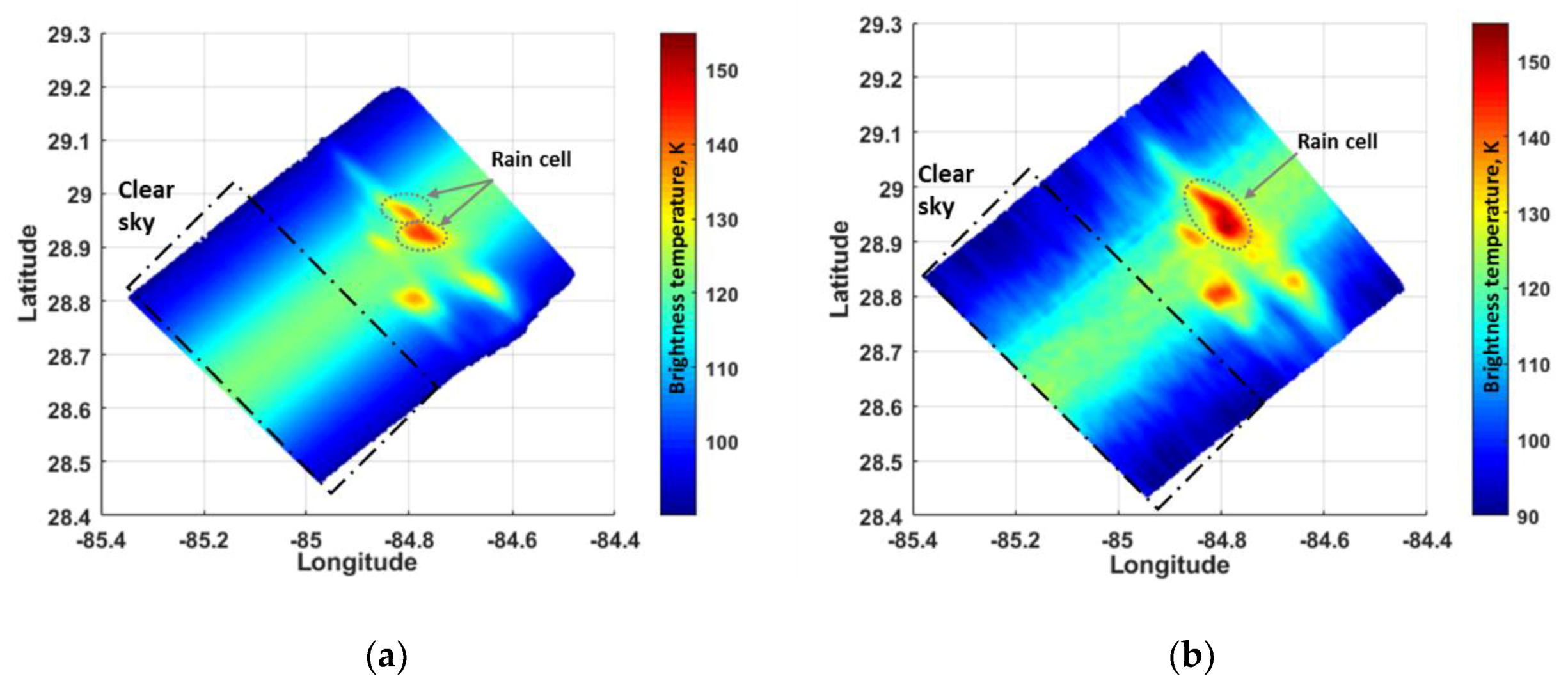
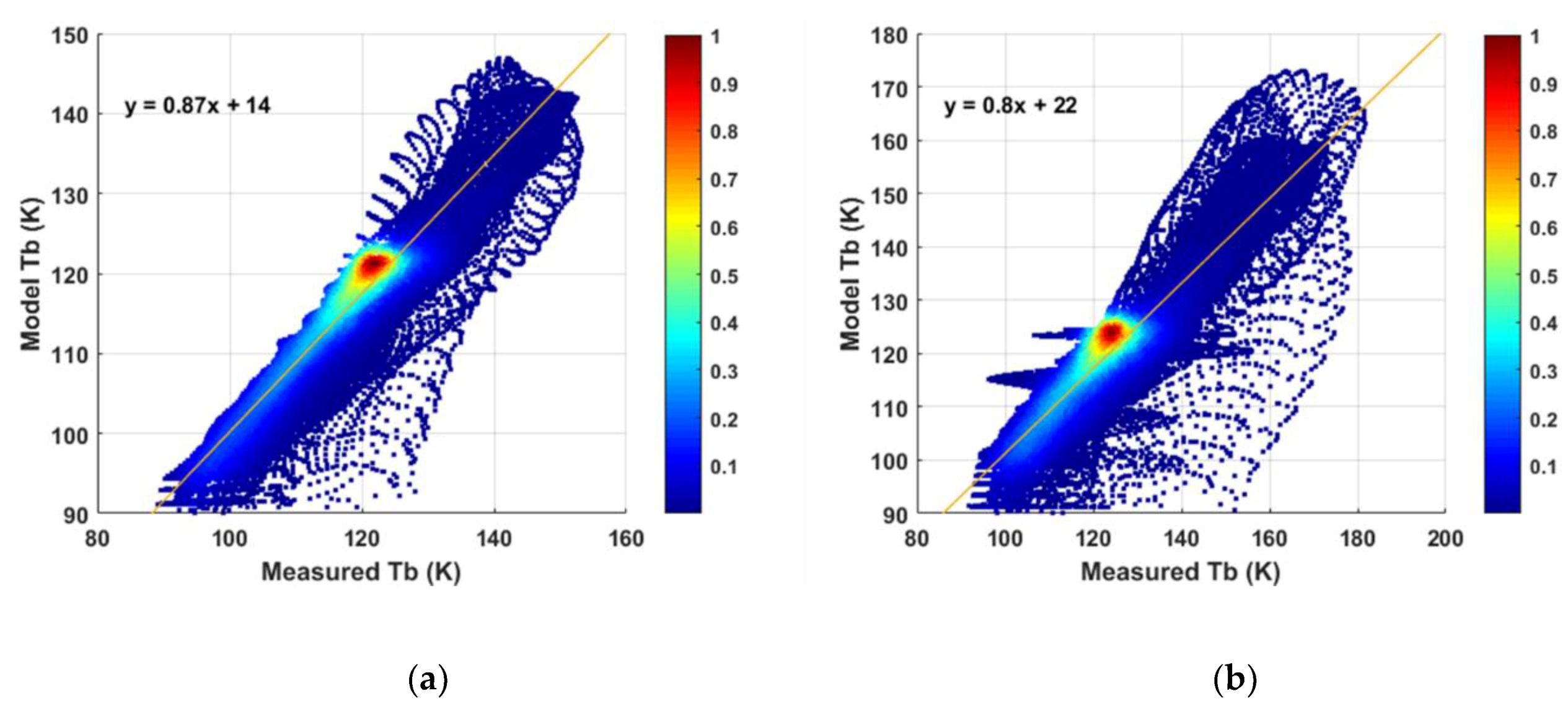
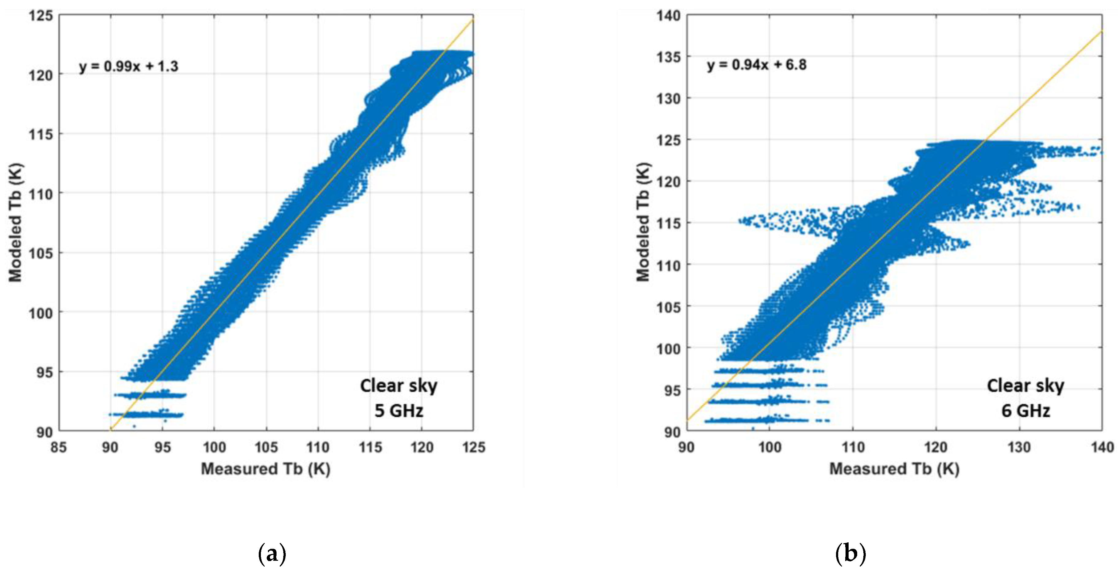
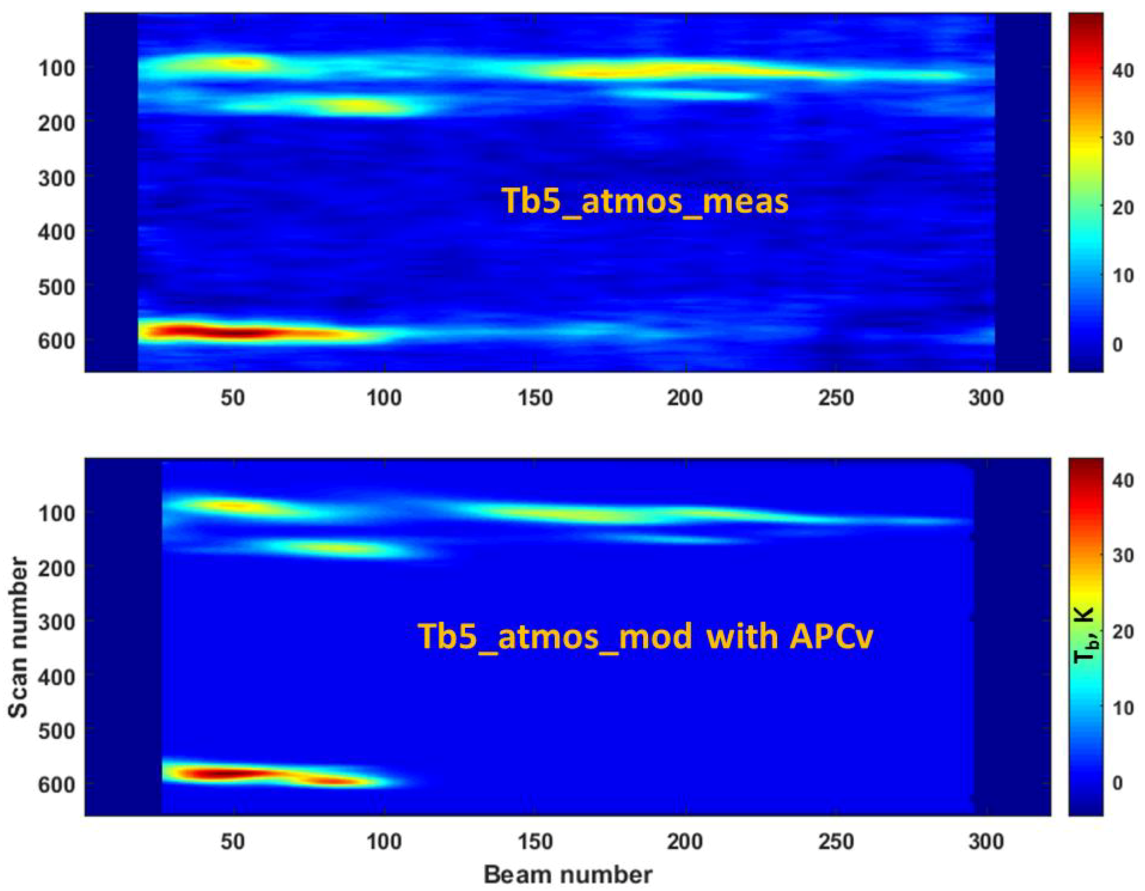
6.2. Comparison of HIRAD Measured and Modeled T_b Images

Comparisons of modeled (left) and measured (right) T_b images are shown in Figure 16 for the tropical squall-line event in the upper half of Global Hawk path-2. First consider the clear-sky region, where the modeled image shows the expected ocean T_b signature of warm T_b in the center that symmetrically decreases in brightness to the edges of swath. Next, considering the measured T_b image (right panel), these two images appear to be equivalent, which is typical of properly calibrated HIRAD ocean T_b images without rain.

Next, examine the modeled image and consider the collection of thunderstorm cells in the squall-line at the beginning of the flight path. There are five distinct convective rain cells that can be identified by the increased T_b (yellow to red colors). Now, compare this modeled rain (T_b) pattern with the corresponding measured HIRAD image, which indicates that the rain features are well represented in both images. Moreover, this indicates that the morphing of the NEXRAD images and the subsequent alignment in time have provided good spatial collocation with the independent HIRAD measurement. To test this hypothesis, the procedure was repeated by co-registering the different NEXRAD volume scan levels without employing the morphing procedure, and the results (not shown) were significantly degraded.

On the other hand, there were some differences between the modeled and measured, which are important. For example, in the modeled T_b image between 29.0° and 28.9° latitude, there are three convective rain cells; however, in the corresponding location of the measured image, there appear to be only two. Thus, the measured T_b image appears to be smoothed compared to the higher contrast modeled image, which is expected because the measured brightness (T_ant) is a sum of all brightness incident on the antenna that are weighted by the HIRAD synthesized beam antenna gain pattern [19]. The resulting measured antenna temperature is the ratio of two double integrals in spherical coordinates ($\theta ,\varphi and \mathsf{\Omega }$), namely:

$$T_{ant}=\frac{{{\displaystyle \iint }}_{4\pi }{T}_{app}\left(\theta ,\varphi \right)\ast F_n\left(\theta ,\varphi \right)\ast d\mathsf{\Omega }}{{{\displaystyle \iint }}_{4\pi }^{ }{F}_n\left(\theta ,\varphi \right)\ast d\mathsf{\Omega }}$$

(15)

where the numerator is the convolution of the apparent brightness temperature scene (surrounding the antenna) with the normalized antenna directional power gain pattern, $F_n\left(\theta ,\varphi \right)$, over the entire 4π steradians of a sphere, and the denominator is the total power collected by the antenna for a uniform scene = 1 Kelvin. As the pole of the spherical coordinate system is aligned with the antenna look-direction (EIA), the corresponding normalized antenna pattern changes with EIA, as discussed in Section 2.

As a result, the modeled T_b without antenna pattern effects, shown in Figure 16a, represents the apparent scene brightness temperature with the HIRAD grid spatial resolution at the surface of about 150 m; the effective spatial resolution of the synthesized HIRAD measured T_b image (Figure 16b) varies from ~2 km (middle of swath) to ~6 km (swath edge) [20]. Therefore, before making a quantitative comparison between modeled and measured T_bs, the antenna pattern convolution (APCv) was performed (using the modeled T_bs), and the spatial resolution was degraded to ~1 km along track and ~2.5 km cross-track.

First, using all pixels in pass-2, scatter diagrams were produced for 5 and 6 GHz between measured and modeled (with APCv applied) T_bs, and the results are shown in Figure 17. In these comparisons, the points associated with clear-sky lay between 90–130 K, and they appear to be “tightly” grouped along the linear regression line. On the other hand, at higher T_bs (associated with rain), there was considerably more divergence and the appearance of multiple paths for the grouping of points, which is an indication of spatial misregistration of rain cells in the two images.

To test this hypothesis, the matrix difference (between the measured and modeled T_bs) was plotted in Figure 18, where the color scale is the corresponding T_b difference in Kelvin. The appearance of coupled blue (negative T_b) and red (positive T_b) patterns in the rainy regions is evidence that these two images were not identical. Nevertheless, the linear regressions tended to average the comparisons and the results for both 5 and 6 GHz scatter diagrams were very good with slopes close to one and small offsets of a few K (see

Table 1. (a) Comparisons of measured and modeled T_bs for 5 GHz, (b) Comparisons of measured and modeled T_bs for 6 GHz.

(a)
Region Pass-2	Model Tb Dynamic Range Max/Min, K	Measurement—Model_APC Mean/STD, K	Regression Slope/Offset
All points scans (1:661)	150/90	1.60/2.76	0.90/1.39
Clear-sky scans (230:530)	130/90	0.25/1.06	0.98/2.14
Rain–1 scans (50:170)	150/100	3.67/3.52	0.90/8.97
Rain–2 scans (550:620)	160/100	4.04/3.44	0.91/7.00
Tb_atmos (R-1 and R-2)	60/8	7.25/1.75	0.77/7.60
(b)
Region Pass-2	Model Tb Dynamic Range Max/Min, K	Measurement—Model_APC Mean/STD, K	Regression Slope/Offset
All points scans (1:661)	150/90	2.22/4.39	0.86/4.5
Clear-sky scans (230:530)	130/90	0.49/2.50	0.88/13.9
Rain–1 scans (50:170)	100/170	4.52/5.27	0.92/5.34
Rain–2 scans (550:620)	100/190	6.43/5.72	1.06/-14.0
Tb_atmos (R1 and R2)	80/8	3.83/2.92	0.78/9.50

at the end of this section). Since no normalization of the modeled nor measured rain rate magnitudes have been made in this comparison, this is a very significant finding, which implies that both the Z-R relation for the NEXRAD and the SFMR derived rain absorption coefficients are in good agreement.

Therefore, pass-2 was partitioned into three regions, namely: “rain-1” (scans 50 to 200), “clear-sky” (scans 230 to 530), and “rain-2” (scans 550 to 620). Consider first the scatter diagrams for the clear-sky region, shown in Figure 19 for 5 and 6 GHz, where the co-registration of measured and modeled images is not an issue. For both cases, there was excellent agreement and the regression results are summarized in Table 1.

Next, the two rain regions were examined separately, and the image 2D cross-correlation functions were performed. For the rain-1 image, the maximum correlation was 88.9% at zero lag in the beam and scan dimensions. On the other hand, for the rain-2 region, the measured T_b around scan 580 showed a band of moderate rain (10–15 mm/h) between beams 100–200, which was missing from the model T_b (i.e., this rain band was not detected by NEXRAD). Thus, the rain-2 image was truncated to cover only the first 100 beams, and the corresponding cross-correlation was calculated, which resulted in a 74.4% maximum, which occurred at lags of five beams and two scans that corresponded to <1 km misregistration. Based upon these results, it was concluded that the size, shapes, and locations of individual rain cells were not a perfect match, but the resulting scatter diagrams given in Figure 20 showed good statistical agreement, and the regression results (as well as results for 6 GHz) are summarized in Table 1.

Next, the average clear-sky brightness component of TOA T_b was removed using Equation (14), and the several comparisons were made between the measured and modeled T_b components due to rain $\mathsf{\Delta }{T}_{atmos\_rain}$ (over the flight pass-2. First, to match the spatial resolution of these two images, the APCv was applied to the modeled data, and the resulting images (in matrix format) for 5 GHz are shown in Figure 21. Note that there is a high degree of spatial correlation in the rain patterns for these two images; but the magnitudes of the rain T_bs were slightly different, as indicated by the RR color scales.

Furthermore, to examine the small-scale structure of the rain-1 region, two cross-track T_b profiles of $\mathsf{\Delta }{T}_{atmos\_rain}$ for the 5 and 6 GHz channels are given in Figure 22. In panel (a), the measured (solid line) and modeled (dashed line) atmospheric T_b components are presented for 5 GHz, and in panel (b), the corresponding plots are given for 6 GHz. For both plots, the spatial variability of the rain features are highly correlated; even though the measured and modeled curves had a small bias (<10 K), this is a minor issue that could have been caused by a number of factors that include sensor calibration errors and collocation issues associated with the heterogeneous nature of the propagating squall-line of thunderstorms.

Additional comparisons between these $\mathsf{\Delta }{T}_{atmos\_rain}$ components (for both 5 GHz and 6 GHz) are presented in Figure 23 in the form of two scatter diagrams with linear regressions applied. As discussed previously, the relatively large spread in these scatter diagrams was probably due to the imperfect co-registration of NEXRAD and HIRAD measurements, but the linear regressions showed good agreement in the mean. Overall, after taking all factors into consideration, these independent comparisons indicate that the HIRAD forward RTM worked very well.

The results for four different cases of comparisons of measured and modeled TOA T_bs are summarized in Table 1 as well as a single case for the comparisons of the measured and modeled atmospheric T_b component due to rain. This table provides pertinent statistics for different spatial regions, which includes T_bs in clear-sky and rainy regions (at the beginning and end of flight pass-2).

7. Discussion

During this Tampa Bay Rain Experiment, a propagating squall-line of thunderstorms was observed by HIRAD operating on the Global Hawk aircraft, and the associated rain surface truth was derived from independent, ground-based NOAA NWS NEXRAD volume-scan radar reflectivity measurements. As the HIRAD and NEXRAD observations were not simultaneous, the analysis of these datasets was challenging to create an instantaneous 3D rain volume dataset. Based upon CFRSL previous experience with NEXRAD reflectivity morphing [12], a signal processing procedure was applied that resulted in a time series (once per minute) of 3D rain volumes with a spatial resolution of a 1.5 km cube. These data were the rain rate environmental input to the RTM and were used to calculate the modeled (top of the atmosphere) T_bs, which were simultaneous and spatially collocated with the HIRAD measurements.

Given this collocated T_b dataset, the next analysis procedure was to calibrate the HIRAD measured T_b images at 5 and 6 GHz. Fortunately, there were two external T_b scenes (clear-sky ocean and uniform land), which were used to provide the radiometric calibration. After applying this calibration, the resulting 5 and 6 GHz measured brightness images were compared to corresponding modeled images for both clear-sky and rainy scenes.

Overall, there was an excellent qualitative comparison showing nearly identical rain images (feature shapes and relative intensities), but there were minor registration differences noted between the corresponding measured and modeled images. However, in previous research [20], the geolocation for the HIRAD T_b image pixels (at the surface) were shown to be accurate within ±1 km; therefore, the geometry portion of the RTM, which calculates the antenna beam’s LOS, is not a significant contributor to the observed rain feature mis-registrations. Moreover, given that the NEXRAD rain rate surface truth is not perfect, it is reasonable that differences in the observed rain feature locations may be attributed to the NEXRAD measurements or subsequent morphing results, and not associated with the HIRAD RTM modeled results.

Concerning the quantitative comparisons, the various sets of statistical evaluations summarized in Table 1a,b are very good. The fact that the slopes of the various linear regressions were close to unity and the offsets were also small is very significant. This implies that both the Z-R relation for NEXRAD (rain rates input to RTM) and the SFMR derived rain absorption coefficients (used in the RTM) are in good agreement. Furthermore, it is important to note that the magnitude of the rain brightness temperature is proportional to the integral of the rain rate along the upwelling and downwelling paths, and that for these comparisons, no normalization of either the NEXRAD rain rates (used in the RTM) nor the measured HIRAD brightness temperatures have been made (i.e., they are totally independent).

8. Conclusions

The results of this paper are significant because they represent the first validation of the HIRAD forward radiative transfer model calculation of brightness temperature for strong convective rain cells. Based upon the empirical comparison of HIRAD measured and modeled results, it can be concluded that the HIRAD RTM performs very well in modeling the TOA brightness temperature of both clear-sky ocean scenes and ocean scenes with convective rain cells. This RTM validation is significant because it becomes the basis for proceeding with the future development of a rain rate retrieval algorithm for HIRAD.

While the NEXRAD rain rate surface truth is not perfect, it is more than sufficient to yield convincing evidence that the RTM preforms well. Overall, the qualitative comparison are highly supportive of the conclusion that given an accurate 3D atmospheric distribution of rain rate (surface truth), the HIRAD forward RTM calculates realistic values of T_b at the top of the atmosphere. Furthermore, the results of the various statistical analyses (given in Table 1) implies that both the Z-R relation for NEXRAD and SFMR derived rain absorption coefficients are in good agreement with the HIRAD measured T_bs. Additionally, it is important to note that HIRAD and NEXRAD measurements are totally independent.

In summary, we conclude that the resulting slight differences (between the measured and modeled T_b images) did not significantly impact the study conclusions. While we recognize that it is not possible to partition these differences into surface truth errors and RTM errors; nevertheless, the resulting comparisons were quite good and more than sufficient to conclude that the RTM performs very well. Therefore, the HIRAD forward RTM, under conditions of strong tropical rains, is validated to provide high quality images of the TOA brightness. This is a necessary step toward to the development of a HIRAD rain geophysical model function (GMF), which will be accomplished using future Monte Carlo simulations with wind and rain field environmental inputs from numerical hurricane models. Once this rain GMF is established, then the development of a rain rate retrieval algorithm for HIRAD can proceed.

References

1. Amarin, R.A.; Jones, W.L.; El-Nimri, S.F.; Johnson, J.W.; Ruf, C.S.; Miller, T.L.; Uhlhorn, E. Hurricane Wind Speed Measurements in Rainy Conditions using the Airborne Hurricane Imaging Radiometer (HIRAD). IEEE Trans. GeoSci. Remote Sens. 2012, 50, 180–192. [Google Scholar] [CrossRef]
2. Uhlhorn, E.W.; Black, P.G.; Franklin, J.L.; Goldstein, A.S. Hurricane Surface Wind Measurements from an Operational Stepped Frequency Microwave Radiometer. Mon. Weather Rev. 2007, 135, 3070–3085. [Google Scholar] [CrossRef]
3. Jones, W.L.; Zec, J.; Johnson, J.W.; Ruf, C.; Bailey, M.C. A Feasibility Study for a Wide-Swath, High Resolution, Airborne Microwave Radiometer for Operational Hurricane Measurements. In Proceedings of the IEEE IGARSS 2002, Toronto, ON, Canada, 24–28 June 2002. [Google Scholar]
4. Johnson, J.W.; Amarin, R.A.; El-Nimri, S.F.; Jones, W.L. A Wide-Swath, Hurricane Imaging Radiometer for Airborne Operational Measurements. In Proceedings of the IEEE IGARSS 2006, Denver, CO, USA, 28 August–1 September 2006. [Google Scholar]
5. Amarin, R. Hurricane Wind Speed and Rain Rate Measurements Using the Airborne Hurricane Imaging Radiometer (HIRAD). Ph.D. Thesis, University of Central Florida, Orlando, FL, USA, 2010. [Google Scholar]
6. Jacob, M.M.; Salemirad, M.; Jones, W.L.; Biswas, S.; Cecil, D. Validation of Rain Rate Retrievals for the Airborne Hurricane Imaging Radiometer (HIRAD). In Proceedings of the IEEE IGARSS 2015, Milan, Italy, 27–31 July 2015. [Google Scholar]
7. Braun, S.A.; Newman, P.A.; Heymsfield, G.M. NASA’s Hurricane and Severe Storm Sentinel (HS3) Investigation. Bull. Am. Meteor. Soc. 2016, 97, 2085–2102. [Google Scholar] [CrossRef]
8. Ruf, C.S.; Swift, C.T.; Tanner, A.B.; Le Vine, D.M. Interferometric synthetic aperture microwave radiometry for the remote sensing of the earth. IEEE Trans. Geosci. Remote Sens. 1988, 26, 597–611. [Google Scholar] [CrossRef]
9. Bailey, M.C.; Amarin, R.A.; Johnson, J.; Nelson, P.; James, M.; Simmons, D.; Ruf, C.; Jones, W.L.; Gong, X. Multi-Frequency Synthetic Thinned Array Antenna for the Hurricane Imaging Radiometer. IEEE AP-S Trans. Antennas Propag. 2010, 58, 2562–2570. [Google Scholar] [CrossRef]
10. Federal Meteorological Handbook No. 11: Doppler Radar Meteorological Observations, Part B: Doppler Radar Theory and Meteorology; Report FCM-H11B-1990, Interim Version One; Office of the Federal Coordinator for Meteorological Services and Supporting Research: Rockville, MD, USA, 1990; p. 228.
11. Fulton, R.A.; Breidenbach, J.P.; Seo, D.J.; Miller, D.A.; O’Bannon, T. The WSR-88D rainfall algorithm. Weather Forecast. 1998, 13, 377–395. [Google Scholar] [CrossRef]
12. Schneider, L.; Jones, W.L. Analysis of spatially and temporally disjoint precipitation datasets to estimate the 3D distribution of rain. In Proceedings of the IEEE IGARSS 2017, Fort Worth, TX, USA, 23–28 July 2017. [Google Scholar]
13. El-Nimri, S. Development of An Improved Microwave Ocean Surface Emissivity Radiative Transfer Model. Ph.D. Thesis, University of Central Florida, Orlando, FL, USA, 2010. [Google Scholar]
14. El-Nimri, S.F.; Jones, W.L.; Uhlhorn, E.; Ruf, C.; Johnson, J.; Peter, B. An Improved C-Band Ocean Surface Emissivity Model at Hurricane-Force Wind Speeds over a Wide Range of Earth Incidence Angles. IEEE Geosci. Remote Sens. Lett. 2010, 7, 641–645. [Google Scholar] [CrossRef]
15. Klotz, B.W.; Uhlhorn, E.W. Improved Stepped Frequency Microwave Radiometer Tropical Cyclone Surface Winds in Heavy Precipitation. J. Atmos. Ocean. Technol. 2014, 31, 2392–2408. [Google Scholar] [CrossRef]
16. Ruf, C.; Roberts, J.B.; Biswas, S.; James, M.; Miller, T. Calibration and image reconstruction for The Hurricane Imaging Radiometer (HIRAD). In Proceedings of the IEEE IGARSS 2012, Munich, Germany, 22–27 July 2012. [Google Scholar]
17. Alasgah, A.; Jacob, M.; Jones, W.L. Removal of Artifacts from Hurricane Imaging Radiometer Tb Images. In Proceedings of the IEEE 2017 SoutheastCon, Concord, NC, USA, 3 March–2 April 2012. [Google Scholar]
18. National Centers for Environmental Prediction (NCEP); Final (FNL). Operational Global Analyses. Available online: http://rda.ucar.edu/datasets/ds083.2 (accessed on 30 April 2019).
19. Ulaby, F.; Long, D. Microwave Radar and Radiometric Remote Sensing; Univ. Mich Press: Ann Arbor, MI, USA, 2014; pp. 236–239. ISBN 978-0-472-11935-6. [Google Scholar]
20. Sahawneh, S.; Jones, L.; Biswas, S.; Cecil, D. HIRAD Brightness Temperature Image Geolocation Validation. IEEE Geosci. Remote Sens. Lett. 2017, 14, 1908–1912. [Google Scholar] [CrossRef]
Figure 1. Typical hurricane surveillance (Fig-4 flight pattern) for SFMR measurements (red trace) from a hurricane hunter aircraft. Additionally, shown are corresponding HIRAD measurements (brightness temperature images) from a coordinated second high-altitude aircraft.
Remotesensing 11 02650 g001
Figure 2. HIRAD equivalent push-broom radiometer measurement geometry with EIA’s of ± 60°.
Remotesensing 11 02650 g002
Figure 3. KTLH NEXRAD rain reflectivity image of a tropical squall-line and the corresponding ground track for the Global Hawk aircraft (shown in red).
Remotesensing 11 02650 g003
Figure 4. NEXRAD rain rate CAPI-1.75 km bounded by the HIRAD swath for the Global Hawk pass-2, with the color-bar indicating rain rate in mm/h.
Remotesensing 11 02650 g004
Figure 5. HIRAD 3D grid for rain rate.
Remotesensing 11 02650 g005
Figure 6. NEXRAD RR images for (a) NEXRAD CAPI RTM L-3 for pass-2 with the location of scan—100 denoted by the dashed red line, and (b) corresponding NEXRAD RR Profile for HIRAD scan—100. Note that both plots are matrix format with different RR color scales.
Remotesensing 11 02650 g006
Figure 7. HIRAD RTM geometry with separate upwelling (blue) and downwelling (red) paths from Amarin [1].
Remotesensing 11 02650 g007
Figure 8. Theoretical clear-sky, TOA, Ocean Tb for HIRAD at 5 GHz (solid curves) and 6 GHz (dashed curves) for fixed WS of 10 (blue), 20 (red), and 30 (black) m/s.
Remotesensing 11 02650 g008
Figure 9. Theoretical HIRAD TOA, Ocean Tb for uniform rain rates at 5 and 6 GHz and three EIA’s.
Remotesensing 11 02650 g009
Figure 10. HIRAD Tb measurements for 5 GHz in (a) raw Tbs; (b) recalibrated Tbs; (c) difference between raw and adjusted Tbs; and (d) average ocean Tb in the “clear-sky box” for raw (dashed) and calibrated (solid).
Remotesensing 11 02650 g010
Figure 11. HIRAD Tb measurements for 6 GHz in (a) raw Tbs; (b) recalibrated Tbs; (c) difference between raw and adjusted Tbs; and (d) average ocean Tb in “clear-sky box” for raw (dashed) and calibrated (solid).
Remotesensing 11 02650 g011aRemotesensing 11 02650 g011b
Figure 12. HIRAD Tb measurements for 6.6 GHz in (a) raw Tbs; (b) recalibrated Tbs; (c) difference between raw and adjusted Tbs; and (d) average ocean Tb in “clear-sky box” for raw (dashed) and calibrated (solid).
Remotesensing 11 02650 g012
Figure 13. Panel (a) is the NEXRAD rain rate profile (color bar in mm/h) with HIRAD upwelling and downwelling LOS paths displayed for the selected beam# 225, and panel (b) shows the corresponding rain rates in RTM layers for upwelling (blue) and downwelling (red) paths.
Remotesensing 11 02650 g013
Figure 14. Theoretical TOA Tb for 5 GHz (upper panel) and 6 GHz (lower panel) for pass-2 of the Tampa Bay Rain Experiment. Note that except for the color bar scales, the images are identical.
Remotesensing 11 02650 g014
Figure 15. Theoretical differential atmospheric rain component of TOA Tb ( Δ T a t m o s _ r a i n ) at 5 GHz for pass-2, with color bar in Kelvin.
Remotesensing 11 02650 g015
Figure 16. Comparison of 5 GHz modeled (a) and measured (b) HIRAD TOA Tb images of the tropical squall-line for the upper half of Global Hawk path-2.
Remotesensing 11 02650 g016
Figure 17. Comparison of HIRAD measured and modeled (with APCv applied) Tb images for pass-2, panel (a) 5 GHz and panel (b) 6 GHz, where the color represents the relative number of points.
Remotesensing 11 02650 g017
Figure 18. Matrix of HIRAD measured minus modeled (with APCv applied) Tb images for the flight pass-2, where the color represents the Tb difference in K.
Remotesensing 11 02650 g018
Figure 19. Comparison of measured and modeled Tbs for the clear-sky region of pass-2 for 5 and 6 GHz.
Remotesensing 11 02650 g019
Figure 20. Comparison of measured and modeled Tbs for the rainy regions (1 and 2) of pass-2 for 5 GHz.
Remotesensing 11 02650 g020
Figure 21. Differential atmosphere brightness component because of rain (matrix format) for 5 GHz. Upper panel is HIRAD measured and lower panel is modeled with APCv applied.
Remotesensing 11 02650 g021
Figure 22. Comparisons of the small-scale rain features in the cross-track differential rain atmosphere brightness components for scan 110 for: (a) 5 GHz and (b) 6 GHz.
Remotesensing 11 02650 g022
Figure 23. Comparison of measured and modeled differential rain atmosphere brightness components for Global Hawk pass-2 for: (a) 5 GHz and (b) 6 GHz.
Remotesensing 11 02650 g023