Article

Using Multi-Sensor Satellite Images and Auxiliary Data in Updating and Assessing the Accuracies of Urban Land Products in Different Landscape Patterns

1
State Key Laboratory of Resources and Environmental Information System, Institute of Geographic Sciences and Natural Resources Research, Chinese Academy of Sciences, Beijing 100101, China
2
University of Chinese Academy of Sciences, Beijing 100049, China
3
Jiangsu Centre for Collaborative Innovation in Geographical Information Resource Development and Application, Nanjing 210023, China
4
Geological Engineering and Institute of Surveying and Mapping, Chang’an University, Xi’an 710054, China
*
Author to whom correspondence should be addressed.
Remote Sens. 2019, 11(22), 2664; https://doi.org/10.3390/rs11222664
Submission received: 17 September 2019 / Revised: 6 November 2019 / Accepted: 13 November 2019 / Published: 14 November 2019
(This article belongs to the Section Urban Remote Sensing)

Abstract

:
Rapid and accurate updating of urban land areas is of great significance to the study of environmental changes. Although there are many urban land products (ULPs) at present, such as GlobeLand30, Global Urban Footprint (GUF), and Global Human Settlement Layer (GHSL), these products are all static data of a certain year, and are not able to provide high-accuracy updating of urban land areas. In addition, the accuracies of these data and their application value in the update of urban land areas need to be urgently proven. Therefore, we proposed an approach to quickly and accurately update urban land areas in the Kuala Lumpur region of Malaysia, and assessed the accuracies of urban land products in different urban landscape patterns. The approach combined the advantages of multi-source data including existing ULPs, OpenStreetMap (OSM) data, Landsat Operational Land Imager (OLI), and Phased Array type L-band Synthetic Aperture Radar (PALSAR) images. Three main steps make up this approach. First, the urban land training samples were selected in the urban areas consistent with GlobeLand30, GUF, and GHSL, and samples of bare land, vegetation, water bodies, and road auxiliary data were obtained by GlobeLand30 and OSM. Then, the random forest was used to extract urban land areas according to the object’s features in the OLI and PALSAR images. Last, we assessed the accuracies of GlobeLand30, GUF, GHSL, and the results of this study (ULC) by using point and area validation methods. The results showed that the ULC had the highest overall accuracy of 90.18% among the four products and could accurately depict urban land in different urban landscapes. The GHSL was the second most accurate of the four products, and the accuracy in urban areas was much higher than that in rural areas. The GUF had many omission errors in urban land areas and could not delineate a large area of complete spatial information of urban land, but it could effectively extract scattered residential land with small patches. GlobeLand30 had the lowest accuracy and could only express rough, large-scale urban land. The above conclusions provide evidence that ULPs and the approach proposed in this study have a great application potential for high-accuracy updating of urban land areas.

Graphical Abstract

1. Introduction

Economic development and population growth lead to the rapid expansion of urban land causing a reduction in the area of other land types, which has an impact on air pollution, water supply, and the ecological environment. Therefore, the accurate and timely update of urban land areas is of vital significance for land cover change measurement, ecological environment protection, and land use planning [1]. For urban planning, information such as the urban structure types, percentage of green areas per block, and brown field management are required in addition to high spatial and temporal resolution urban development maps. At present, there is no uniform definition of urban land. In order to avoid ambiguity, the urban land in this study refers to impervious surfaces, i.e., the areas formed by artificial construction activities such as buildings, settlements, roads, and parking lots, excluding contiguous green land and water bodies in residential areas [2,3].
In the past 10 years, with the rapid development of remote sensing technology, numerous urban land products (ULPs) with high spatial resolution have been published. The main data include FROM-GLC10 from Tsinghua University [4], the GlobeLand30 from the National Geomatics Center of China [5], the Global Urban Footprint (GUF) from the German Aerospace Agency [6], and Global Human Settlement Layer (GHSL) from the European Commission’s Joint Research Centre [7,8]. Except for the last two datasets, which are thematic data of urban land, the other datasets are full-element land cover data. These data have been widely used in urban planning, population density mapping, land use analysis, and other fields [9,10,11,12,13]. However, for the change detection and spatiotemporal pattern analysis of urban land, these static products collected at certain points in time cannot meet the demand. Therefore, it is of great value to have ULPs that are quickly updated and are highly accurate.
One factor that affects rapid ULP updating is the selection of training samples. It is well known that the traditional methods (e.g., visual image interpretation or field survey) of sample selection are time-consuming and laborious. Therefore, many attempts have been carried out to optimize this process by combining remote sensing images and ULPs [14,15]. Although these methods have obtained high-accuracy of urban land data, the results were still dated (from 2010); therefore, the updating of urban land areas has not yet been achieved. By contrast, Gong et al. have acquired the urban land areas in 2017 through the transfer of past samples [4]. However, their method only uses the atmospheric bands of Sentinel 2, and therefore a single data source cannot meet the demand of extracting urban land areas in complex landscapes. For example, it is difficult to distinguish between urban land areas and bare lands simply based on the spectral information. In this regard, Zhang et al. proposed to comprehensively use the spectral information and multivariate texture of Landsat images, and obtained the urban land data with an accuracy of 92.35% [16]. But in tropical, subtropical, and other cloudy areas, high-quality optical images are difficult to obtain. Previous studies have shown that radar images could solve these problems to a large extent [17,18,19,20]. In terms of the spatial resolution of the images used, although Berger et al.’s study has shown that the use of high spatial resolution multi-spectral data and light detection and ranging data can obtain fine urban land data [21], the huge amount of data, high cost, and time-consuming calculation make the application of such data difficult [22]. A large number of studies have proven that medium-high spatial resolution images, such as the Landsat Operational Land Imager (OLI) and Phased Array type L-band Synthetic Aperture Radar (PALSAR), have rich classification features and are often used for urban land mapping and urban dynamic change detection [17,18,19,23]. Therefore, to improve the accuracy and efficiency of urban land areas extraction, OLI and PALSAR images were used in this study. In addition, OpenStreetMap (OSM) data containing a large amount of land use information are available in most areas. So, it is a data source for land cover/land use research with high practical value and high accuracy [24,25,26]. Thus, we attempted to combine the advantages of multi-source data to update urban land products quickly and accurately.
Although there have been some research advances in the accuracy analysis of ULPs with high spatial resolution (GlobeLand30, GUF and GHSL), these conclusions are the evaluation of the overall accuracy and do not fully consider the strengths and weaknesses in different urban landscapes [14,27,28]. The lack of a comprehensive accuracy verification and comparative research is one of the main reasons that prevent users from using these data products more widely, effectively, and objectively. The research on the accuracy variation of each ULP across regions of varying development intensities and the difference comparison between different ULPs is particularly scarce. In order to make better use of these data, it is necessary to assess the accuracy of each ULP in various urban areas (urban clusters, scattered settlements, and small villages). In this regard, we used the method of point validation and area validation to comprehensively compare and analyze the accuracy of each ULP in the large-scale Kuala Lumpur region with varying landscape characters.
The objectives of this study are: (1) to develop a method to quickly and accurately update urban land areas using the existing high spatial resolution ULPs (GlobeLand30, GUF, and GHSL), OSM data, Landsat OLI, and PALSAR images; and (2) to evaluate the strengths and weaknesses of different ULPs. First, in order to solve the problem of the time-consuming and labor-intensive process of training sample acquisition, a method of using existing ULPs and OSM data to select training samples was used. Then, a random forest classifier was used to classify urban land according to the optical characteristics of OLI and the scattering information and texture features of PALSAR. Finally, point accuracy validation and area accuracy validation methods were used to evaluate and analyze the results of this study as well as the accuracy of the existing ULPs (GlobeLand30, GUF, and GHSL). Then the strengths and weaknesses of each product in different landscapes were revealed and discussed.

2. Materials and Methods
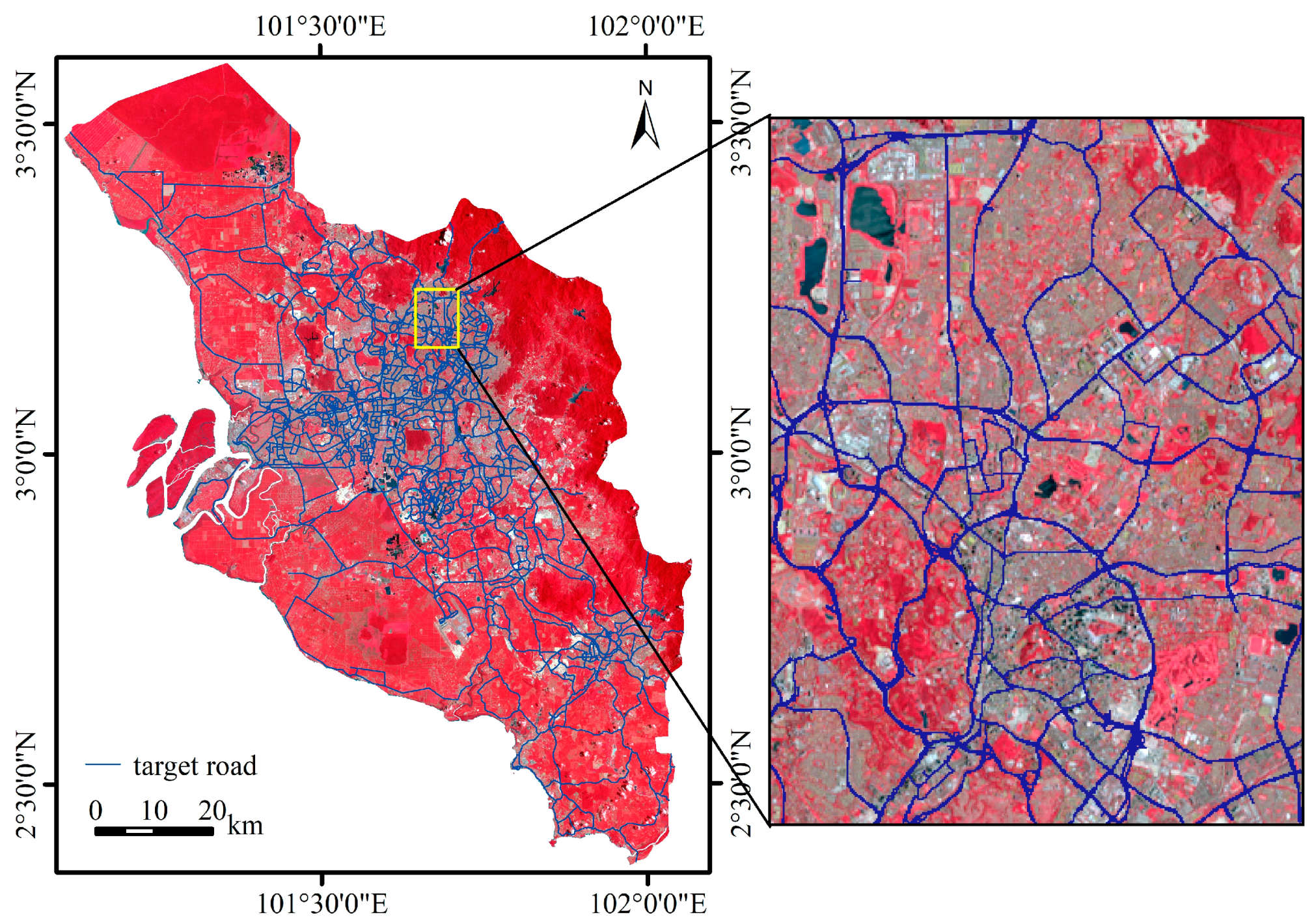
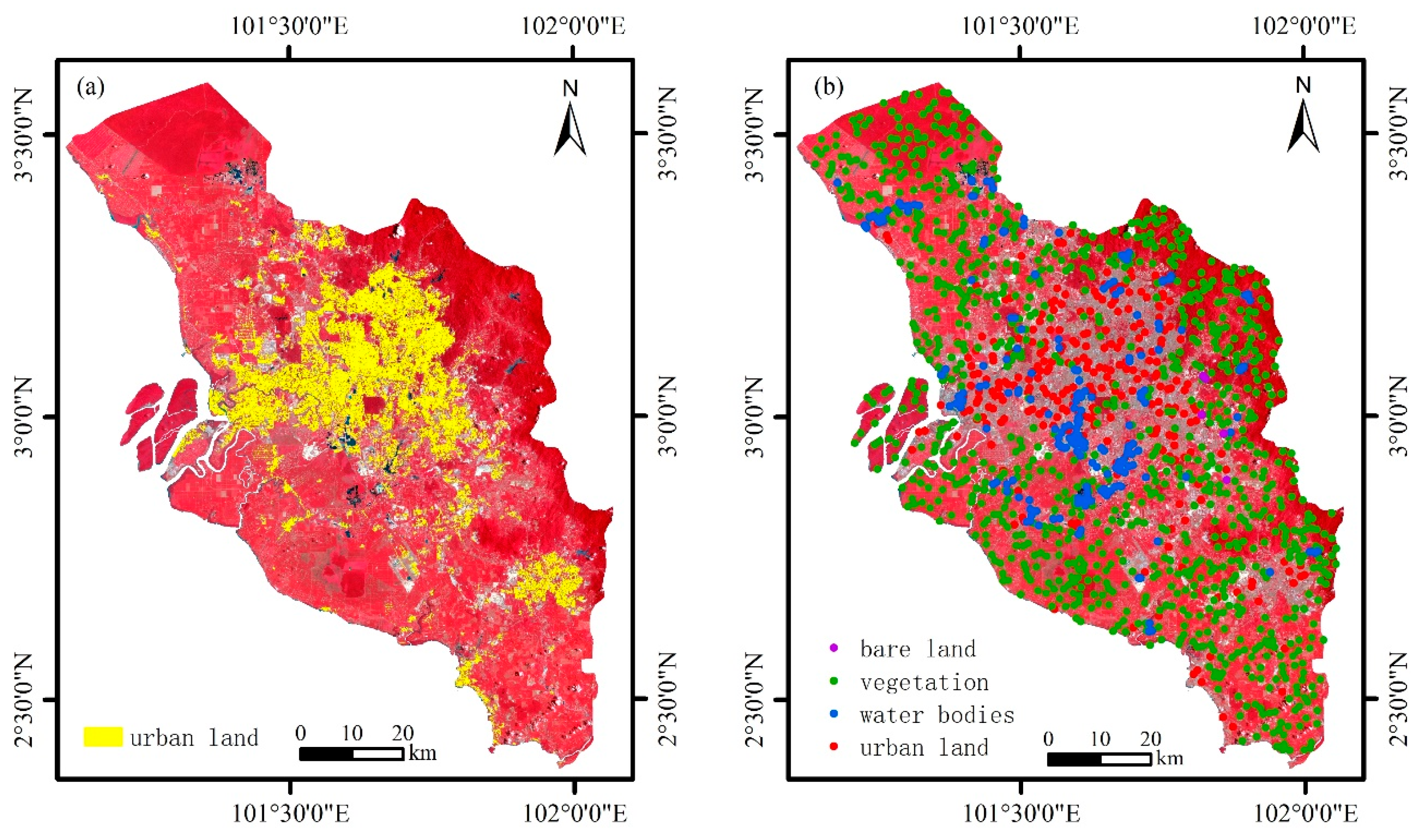
2.1. Study Area

Kuala Lumpur, Malaysia, and its surrounding areas were selected as the study area, comprising two federal territories, Kuala Lumpur and Putrajaya, and eight districts, namely, Port Dickson, Seremban, Gombak, Hulu Langat, Klang, Kuala Langat, Kuala Selangor, Petaling, and Sepang, as shown in Figure 1. The study area is 6994 km2 in total, which includes both large cities with high impermeability, such as Kuala Lumpur, and scattered peri-urban areas with low impermeability. In addition, the study area covers the coastal plain and inland mountainous area, with abundant landscape types. Therefore, it is convenient to detect the robustness of our proposed approach and conduct a comprehensive comparative study. According to the impermeability density, the study area is divided into a high-density urban region (Kuala Lumpur, Petaling, and Klang), medium-density urban region (Putrajaya, Sepang, Hulu Langat, Seremban, and Gombak), and low-density urban region (Port Dickson, Kuala Langat, and Kuala Selangor), as shown in Figure 1a.

2.2. Data and Preprocessing

2.2.1. Urban Land Products

Three ULPs with high spatial resolution (approx.10–40 m) were used in this study and are described in detail below.
The GUF is a global built-up thematic information dataset generated by the German Aerospace Agency using very high-resolution synthetic aperture radar data collected by the TerraSAR-X add-on for Digital Elevation Measurements mission from 2011 to 2013. The research team proposed the Urban Footprint Processor method to extract built-up areas, which mainly includes three steps. First, the texture feature information of highly structured and diversified built-up areas is extracted. Then, based on the backscattering characteristics of the original image and the extracted texture features, an unsupervised classification method is used to generate binary layers, where the high value area is classified as built-up, and the remaining areas are classified as non-built-up. Finally, the extracted data are spliced and processed to generate the global built-up data with a spatial resolution of 12 m. The GUF only contains built-up regions with vertical structures while ignoring impervious surfaces without vertical structures. Therefore, GUF data are prone to omit low building structures such as roads [6,29,30,31].
The GHSL is the global human settlement data for four epochs since 1975 (GLS1975, GLS1990, GLS2000, and GUS2014) and has a spatial resolution of 38 m. Landsat data from the past 40 years were collected to produce these four epochs of data. Urban land, according to the GHSL definition, refers to an area covered by buildings. A new supervised classification method based on symbolic machine learning was used to produce the GHSL. Compared with other global data obtained by automatic extraction methods using Earth Observation data, the accuracy of GHSL is higher [7]. In this study, GHSL data from 2014 were used to make up for the absence of GUF data in non-vertical structures on urban land.
GlobeLand30 is a data product of the 863 Program of the Ministry of Science and Technology of China, called “Global Surface Covering Remote Sensing Mapping and Key Technology Research.” It contains data for the years 2000 and 2010. This study uses the 2010 data from GlobeLand30 with a spatial resolution of 30 m. The classification mainly uses the Landsat Thematic Mapper, the multi-spectral imagery of Landsat 7 Enhanced Thematic Mapper Plus, known as ETM+, and imagery from the Chinese Environmental and Disaster satellite, HJ-1. The existing land cover data, MODIS NDVI data, global basic geographic information data, global DEM data, various thematic data, and online high-resolution images are used as auxiliary data. The classification results are obtained by pixel- and object-based methods with knowledge. The artificial surface of the dataset refers to the surface formed by artificial construction activities, including various residential areas such as towns, industrial and mining areas, and transportation facilities, excluding the contiguous green land and bodies of water within construction land. Compared with GUF and GHSL, GlobeLand30 contains more comprehensive information of the impervious surfaces. Moreover, GlobeLand30 is the world’s first full-element global land cover dataset that has a 30-m resolution and a high overall accuracy (OA) of 83.51%, which could provide various types of sample information [5].
For subsequent classification and comparative analysis, the above three products uniformly adopted the Universal Transverse Mercator projection and Datum World Geodetic System 84.

2.2.2. Remote Sensing Images and Preprocessing

In this study, a Landsat OLI image taken on 29 March 2016, and 2016 PALSAR mosaic images were used to classify urban land.
We obtained the Landsat optical image with a resolution of 30 m from the USGS. To improve the classification accuracy, topographic correction and radiation correction were applied to the OLI image using ENVI 5.3 software.
PALSAR mosaic images were generated by the Japan Aerospace Exploration Agency. These images contained horizontal-horizontal (HH) and horizontal-vertical (HV) polarization bands at a spatial resolution of 25 m. All the bands were radiation-calibrated, slope-corrected, and orthographical-corrected by the data publisher. The amplitude values of HH and HV were converted to gamma naught backscattering coefficients using Equation (1) [32]:
γ0 = 10 × log10DN2 − 83,
where γ0 is the backscattering coefficient and DN is the amplitude value of the image. To reduce speckles, a 3 × 3 pixel median filter was applied on the HH and HV bands. In addition, this study used the nearest-neighbor method to resample all the bands to 30 m and re-projected to the Universal Transverse Mercator projection and Datum World Geodetic System 84 to match the Landsat OLI images. Many studies have shown that the difference (HH–HV) and ratio (HH/HV) of the HH and HV bands can also reflect the ground object category, and thus, they have been widely used for land cover classification. Therefore, the band information of difference (HH–HV) and ratio (HH/HV) were also used in the classification of urban land in this study [20,33].

2.2.3. Open Street Map Data

It is often difficult to obtain continuous roads by image interpretation, leading to the connectivity of roads and the accuracy of urban land being reduced. According to our experience, using OSM data to assist in the extraction of roads may solve this problem. This study used historical road data of OSM from 2016 from the same period of the OLI images. The original road data of OSM are linear vectors with an attribute table. Twenty-five road types are recorded in the attribute table. Trunk roads are generally considered to be more reliable in the road data of OSM, and narrow roads with low levels cannot be expressed in the OLI images with 30 m resolution. Therefore, we selected the records marked as primary, secondary, trunk road, and motorway in the attribute table as the target road area to improve the accuracy of the auxiliary data. Next, an object-oriented method was used to obtain planar road data by combining the OLI images. The OLI images were segmented by the eCognition 9.0 developer software. The scale parameter was set to 5 to obtain small homogenous patches, and the parameters of color, shape, smoothness, and compactness were set to 0.9, 0.1, 0.5, and 0.5, respectively. This study specified that the image patches intersecting the OSM vector data were the target roads, so the feature of the “number of overlapping thematic objects” was used to extract the planar road data. The extraction rule was set to “num. of overlap”: OSM road ≥ 1, and the segmentation object conforming to the rule was the target road. Figure 2 shows the extraction results. It can be seen that the object-oriented method avoided the “salt-and-pepper” problem and ensured the connectivity of the road.

2.3. Training Sample Selection

Different from the previous methods of manual visual sample selection, this study was based on the existing ULPs and open source OLI images to rapidly obtain training samples. To guarantee the authenticity and objectivity of the samples, the stratified random sampling strategy was used. In this way, the training samples of each class would be evenly distributed in large patches and sporadic patches so that the distribution of samples in space is ensured to be reasonable.
It is generally believed that the conversion from urban land to other land cover types rarely occurs [34,35,36]. Therefore, if a certain land parcel was classified as urban land from 2010 to 2014, it is unlikely to have been converted to other land use types in 2016. According to this general assumption, the training samples of urban land were randomly generated in the areas where GUF, GHSL, and GlobeLand30 are all urban land. First, GUF, GHSL, and GlobeLand30 were converted into vector format, and the region where all three are urban land areas was generated by intersection (Figure 3a). The training samples of urban land were randomly generated in this region. The other land cover types in GlobeLand30 were then grouped into three categories, namely, vegetation, water bodies, and bare land. Since the type of wetlands in the study area were mainly mangroves, the cultivated land, forestland, grassland, shrubs, and wetlands were all grouped into the vegetation type, and the remaining two types were water bodies and bare land. Random training samples of corresponding types were generated in the data of vegetation, water bodies, and bare land.
In order to improve the purity of vegetation, water bodies, and bare land samples, an OLI image in 2016 was used to calculate the NDVI and the Modified Normalized Difference Water Index (MNDWI). According to the existing body of knowledge [37,38,39], in most cases, the NDVI of vegetation samples is greater than 0, the MNDWI of water body samples is greater than 0, the NDVI of bare land samples is less than 0.1, the MNDWI of bare land samples is less than 0, and samples that do not meet the rules were excluded. Finally, 264 urban land samples, 230 water body samples, 947 vegetation samples, and 19 bare land samples were generated (Figure 3b).

2.4. Urban Land Classification

In this paper, the land cover types in the study area were classified into bare land, vegetation, water bodies, and urban land, rather than directly into urban land and non-urban land. This avoids classification errors caused by large differences in non-urban land characteristics and could improve classification accuracy. There are three key problems in the object-oriented classification method—the setting of segmentation scale [40,41], the selection of classification features, and the selection of the classifier.
Yang et al.’s classification study in Singapore showed that when using OLI and PALSAR image classification, high classification accuracy could be achieved when the segmentation scale is between 40 and 80 [20]. The location of this study area is close to Singapore, and the land cover type and natural environment conditions are very similar. Therefore, the setting of the segmentation scale may refer to their research conclusions. Under the premise of considering accuracy and efficiency, the segmentation scale of this study was set to 80, and default values were used for other segmentation parameters.
The spectral features of the OLI images and the scattering as well as texture features of the PALSAR images were used in the classification process. Numerous land cover classification studies have indicated that NDVI, MNDWI, and the normalized difference building index (NDBI) could effectively improve the classification accuracy of vegetation, water bodies, and urban land, respectively [2,20,42]. Therefore, in addition to using the spectral mean and standard deviation of each band of Landsat OLI, we also introduced MNDWI, NDVI, and NDBI. The texture features of the HH and HV scattering bands of PALSAR were calculated based on the Gray-Level Co-occurrence Matrix (GLCM), which contained homogeneity, mean, contrast, angular second moment, standard deviation, entropy, dissimilarity, and correlation. All of the classification features were calculated by the eCognition 9.0 developer software based on segmented objects. The features used in this study are shown in Table 1.
This study used the Random Forest classifier to perform the classification. The Random Forest classifier is an ensemble learning algorithm and is quite robust and accurate to noise [43,44]. There are two key parameters to set the decision tree classifier in the eCognition 9.0 developer software, i.e., the number of trees and the minimum number of samples per node [45]. Previous studies have pointed out that using a large number of trees and a small number of the minimum number of samples per node tends to provide better classification results [46]. Therefore, the number of trees was set to 100, and other parameters used default values, considering the time cost.

2.5. Accuracy Assessment

The accuracy is verified in two ways. One is the point accuracy validation. We conducted a nine-day field survey in Malaysia from 29 November to 7 December 2018, and obtained eight urban land and seven non-urban land investigation points located in the study area. Although the survey was conducted in 2018, we consulted local residents to ensure that the land use type of these 15 investigation points had not changed since 2016. With the help of Google high-resolution images in 2016, the remaining 1635 validation points were obtained by stratified random sampling, among which 913 were non-urban land validation points and 652 were urban land validation points. In order to compare the accuracy with other urban land use products, we, respectively, labeled these 1650 validation points with Google high-resolution images from 2010, 2013, and 2014 taken at the same time as GlobeLand30, GUF, and GHSL, so as to obtain the validation points of each product in the same year. The OA, producer’s accuracy (PA), and user’s accuracy (UA) were used as the evaluation indicators [47].
Another verification method is area accuracy validation. We found that the distribution pattern of urban land use in the study area could be divided into three types—scattered distribution along a road, small regional clusters, and large cities. The mixed distribution of urban land and non-urban land in the first two models is easy to generate overestimation and underestimation, and the point accuracy validation cannot explain this area error. In order to fully verify the accuracy of the product, six typical areas that had experienced little change in the urban area since 2010 were selected, as shown in Figure 4. The first row is the type of scattered distribution along the road, and the second row is the small regional cluster. In this study, we zoomed high-resolution Google images to 1:50,000 scale and obtained the real urban land (RUL) in each region through visual interpretation. According to the general knowledge of the profession, the image with meter-level spatial resolution could produce maps with a scale larger than 1:50,000. The highest spatial resolution of all products to be validated in this study is 12 m. Therefore, the RUL obtained at the scale of 1:50,000 is sufficient to meet the accuracy requirements. The area accuracy is defined as the ratio between the area of the intersection of a ULP and RUL and the area of the union of a ULP and RUL. The formula is as follows:
Area   Accuracy = A r e a | R U L U L P | A r e a | R U L U L P | ,
The higher the area accuracy, the higher the classification accuracy, and the closer the classification result is to the real spatial distribution of urban land. On the contrary, it represents that the spatial distribution of ULPs differs greatly from the actual situation, and the product precision is not high.

3. Results

3.1. Urban Land Classification Results

Figure 5d shows the results of the classification of urban land (ULC). It can be seen that urban land is concentrated in the metropolitan area centered in Kuala Lumpur, with the rest grouped in small clusters or along roads. In addition, the urban land of the western coastal areas is clearly greater than that of the eastern mountainous areas, which has a lot to do with the developed economies of the coastal areas. Compared with the other three ULPs in Figure 5, our classification results are the most detailed, especially in terms of road network performance, which is better than that of GlobeLand30 and GUF.
We selected four typical representative regions of different landscape patterns to compare the results we produced with the other three products, as shown in Figure 5 (the blue boxes). These four areas vary in terms of terrain conditions, urban land density, background information, and other aspects, covering various urban land types from large urban agglomerations to scattered villages. Therefore, it is possible to comprehensively analyze the differences between the products and the strengths and weaknesses of the products themselves in different landscape patterns.
The first row in Figure 6 shows the type of large urban agglomeration that has a developed economy and high impermeability. In these areas, water bodies and vegetation within the city are easily misclassified as urban land. The black frame area in Figure 6a is a small patch of green plants inside the city, and the clear overestimation by GlobeLand30 is shown in Figure 6c.
The second row in Figure 6 is representative of piedmont towns, which are generally shown as clusters. The description of GUFs of this type is too fragmented to express spatial semantic information within the urban land and the road. GlobeLand30 overestimates within the towns, but small villages are omitted in the urban-rural transition zone. GHSL and ULC could reveal the spatial details of the interior of this clustered urban land, but ULC is better at depicting the roads and outlines around towns.
The third row is the towns in the plains. Urban land is usually distributed along roads and is often in the form of a grid. GHSL, GlobeLand30, and GUF have left out the scattered settlements within the grid. In addition, GlobeLand30 directly classifies the open land and cultivated land among villages as urban land, and there is a serious overestimation. ULC, by contrast, is more accurate in extracting scattered urban land in this region.
The fourth row is the mountainous urban land type, which is usually scattered in the valley. According to the trend of the valleys, most of the urban land is long and narrow. In addition, the urban land is small and mixed with various background features, making it very difficult to extract. GlobeLand30 and GUF are vastly underestimated in this region. In particular, GlobeLand30 cannot show the urban land of this region at all, while ULC could provide comprehensive spatial information and an outline of urban land.

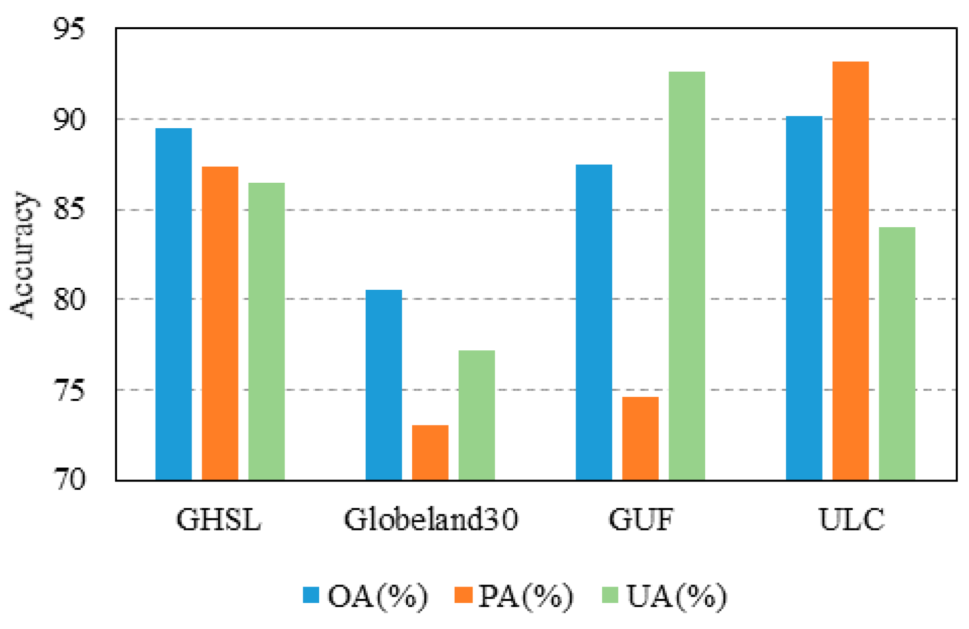
3.2. Point Accuracy Validation and Comparison

We first verified and compared the accuracy of each product using the validation points in the same period as each product. Figure 7 shows the OA, PA, and UA of each product. The OA of GHSL, GlobeLand30, GUF, and ULC was 89.21%, 80.54%, 86.84%, and 90.18%, respectively. It can be seen that the results of the proposed method in this study are superior to the existing data products. The PAs of ULC and GHSL are higher than those of UAs, indicating that the leakage estimation of urban land of these two datasets is less than the error estimation, and there is a certain degree of overestimation. This is probably because the two sets of products are classified by optical images. The bare land with high reflection information in the optical images is most likely to be misjudged as urban land, thus causing overestimation. On the contrary, the PA of GUF is extremely low and the UA is the highest among the four sets of products, indicating that the misclassification is less than the omission, and underestimation exists. GUF is the urban land extracted from radar data based on building height information, so the impact of bare land on the results could be largely excluded. However, it ignores urban land such as roads and parking lots that do not have a vertical structure and therefore produces an underestimation.
In order to obtain the accuracy differences of the four sets of products in areas with different impermeability density, according to the partition of impermeability density in Figure 1a, we calculated the OA of each product in each impervious density level, as shown in Figure 8. From the perspective of different products, the OA in each impervious density level is consistent with the OA of the region. ULC and GlobeLand30 have the highest and lowest accuracy at each density level, respectively. The results indicate that the accuracy of ULC is better than other products in both urban and rural areas, and the performance of this advantage is stable, which further proves the robustness of the approach proposed in this paper.
From the aspect of impermeability density, the accuracy of ULC, GHSL, and GlobeLand30 decreases with the decrease of impermeability density. This indicates that the accuracy of these three products in urban areas is higher than that in rural areas, i.e., the extraction of large urban land patches is better than that of small patches. Therefore, we need to pay attention when using these three products in rural areas. On the contrary, the accuracy of GUF in areas with low impermeability density is clearly higher than that in areas with high impermeability density, indicating that GUF is good at depicting scattered urban land. Therefore, GUF is recommended in rural areas.

3.3. Area Accuracy Validation and Comparison

In order to more accurately analyze the performance of each product in different urban land types, the area validation method introduced in Section 2.5 was adopted to calculate the accuracy of each product in the selected area. The results are shown in Table 2. Among all of the urban land types, ULC had the highest accuracy, while GlobeLand30 had the lowest accuracy, which supports the conclusion in Section 3.2. The accuracy of the clustered urban land was higher than that of road-urban land in the four products. Among them, GlobeLand30 had the greatest difference in accuracy between the two types, and its accuracy of urban land distributed along roads was only 2.37%, indicating that the product has extreme difficulty in depicting small scattered settlements. The accuracy of clustered urban land was about twice that of road-urban land in GHSL and GUF, so it can be seen that for these two products, clusters of small areas of urban land could be expressed more accurately than long strips of urban land distributed along roads. Compared with the first three products, the accuracy difference between these two types of urban land in ULC is not clear. Therefore, among the four sets of products, the method proposed in this study has high extraction accuracy and stable performance in small urban land areas.
However, the accuracy of the area validation method was found to be much lower than that of the point validation method. We believe that there may be three reasons. First, these two types of urban land are located at the border of urban and rural areas or rural areas, with the low density of impermeability rates and complex background land types, making it difficult to extract urban land. This is consistent with the low accuracy in low and medium impermeability density areas verified by the point validation method. Second, the area validation method is used to verify the spatial area difference between the product and the RUL, and the point validation method only verifies the accuracy of the overlapped area with the point. Therefore, the method of area validation should be more rigorous than point validation in theory, and its accuracy is usually lower and closer to the real accuracy of the product. Considering that it is difficult for us to obtain the RUL of the whole research area, only six typical areas were selected for representative analysis. Third, the validation points and RUL produced by manual interpretation may contain error information [48]. Compared with verification points, manual interpretation of the RUL may result in more false labeling due to mixed pixels and fuzzy edge structure, which results in lower area accuracy [49,50,51]. However, in the absence of ground reference data from standard measurements, manual interpretation is a relatively feasible and universal method by which verification reference information is obtained.

4. Discussion

4.1. Issues Related to the Accuracy of Urban Land

According to the analysis in Section 3, the accuracy of the products obtained by the method we propose is the highest among the four products, and better extraction results were achieved in different urban landscapes. This indicates that the method used in this study was able to not only improve the degree of automation of training sample selection but also obtain high-precision urban land with good robustness. It provides a solution for updating urban land areas quickly and accurately.
It should be acknowledged that our products have the same problem of overestimation and underestimation as the other three products. ULC, GHSL, and GlobeLand30 are all produced by remote sensing images with a spatial resolution of 30 m. In these types of medium-resolution images, there are some mixed pixels, and the spectral and texture features of these pixels are often between urban land and non-urban land, easily resulting in misclassification or omission [52]. In addition, for optical images, bright urban land made up of metal or new concrete is easily confused with bare land that has the same high reflective information; and dark urban land made up of asphalt or old concrete is easily confused with water bodies, which have the same low reflection information. The segmentation scale in the production of ULC also affects the accuracy of the products [53,54,55]. Excessive scales could produce mixed objects. If the buildings and the green space between them are divided into one object, it is extremely easy to have overestimation occur. Unlike the other three products, GUF has a large underestimation and very few overestimations. This may be because GUF is generated based on texture information from radar images and is sensitive to buildings with vertical structures, but it ignores roads and flat and open construction land.
Second, it is worth noting that different products have differences in the semantic definitions of urban land, and we selected validation points according to the definition standards of this study, which may reduce the accuracy of existing ULPs. However, this difference in semantic definition does not prevent us from comparing ULPs. On the contrary, by comparing products with unified definition standards, we could fully understand the differences between products and their advantages and disadvantages in the current research, which could guide us to make better use of these data in future research.
Ultimately, one might put forward the question that the time inconsistency of these products would also be a factor that affects the accuracy. To avoid this influence, as described in Section 2.5, we used the validation points that were contemporary with each product. Moreover, the method we proposed is based on current images, so the time-phase difference of data products used is not a problem in this study.

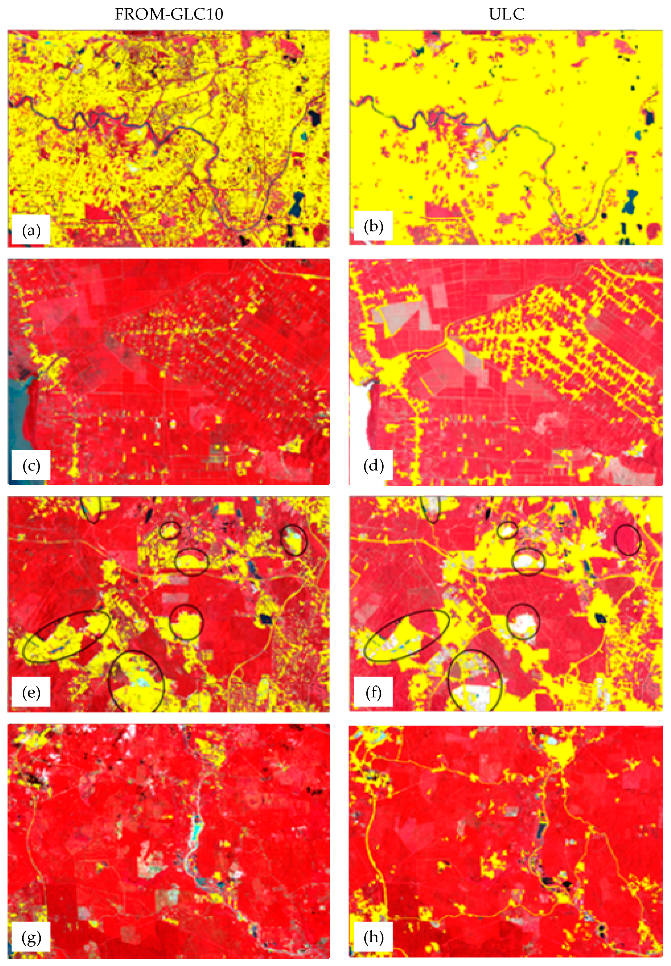
4.2. Comparison of ULC and FROM-GLC10

As mentioned in Section 4.1, the accuracy of ULC is affected by the spatial resolution of the image used. Therefore, we compared ULC with a product with a higher spatial resolution to prove its merits and downsides. FROM-GLC10 is a 10-m resolution global land cover map of 2017 generated by Sentinel-2 data [4]. By comparing ULC and FROM-GLC10, we found that ULC is slightly inferior in the ability to express spatial details than FROM-GLC10 (Figure 9a,b). FROM-GLC10 can clearly depict the block boundaries within the city, while ULC can only depict the urban boundaries of a large area. This may indicate that finer urban land data can be obtained by using images with higher spatial resolution. However, in terms of accuracy, FROM-GLC10 seems to be inferior to ULC. As can be seen from Figure 9c–f, compared with ULC, FROM-GLC10 more easily omits scattered residential land and misclassifies bare land into urban land. This may be due to the fact that ULC is generated from multi-sensor images, that is, radar images make up for the inadequacy of simply using optical images to accurately distinguish between urban land and bare land. In addition, the integration of OSM data improves the accuracy and connectivity of the roads in ULC (Figure 9g–h). Therefore, we can conclude that FROM-GLC10 has a greater application value in urban fine analysis, while ULC has advantages in accuracy.

4.3. Strengths and Weaknesses of Different Urban Land Products

By verifying the accuracy of various products in different urban landscapes, we gained a comprehensive understanding of their strengths and weaknesses. ULC has the highest accuracy and could accurately depict large cities with high impermeability and scattered residents with low impermeability. However, compared with urban areas with dense buildings, its ability to extract urban land in small areas with complex background structure is weak. In addition, we found that ULC has a strong advantage in providing complex outlines of urban land. GHSL is second only to ULC in terms of accuracy, but it is more suitable for expressing a wide range of urban land, depicting the macro-morphology of the city, and has more errors at the pixel level. The accuracy of GlobeLand30 is the lowest among the four sets of products. Small areas of non-urban land within cities are often classified as urban land. Also, its expression ability in rural areas is worse, almost missing the scattered settlements of this region. This is consistent with Sbafizadeh-Moghadam et al.’s conclusion that GlobeLand30 underestimates the size of the urban land [56]. In contrast to the first three products, the accuracy of GUF in low impermeability areas is slightly higher than that in high impermeability areas. Clearly, underestimation exists in the urban areas, but the accuracy of the urban suburbs is relatively high. In terms of urban form expression, GUF is too fragmented to accurately show the urban contour. To summarize, when analyzing urban land use, we recommend the results obtained by this study. For existing products, GHSL is more suitable for use in urban areas, and GUF could fill in for the deficiency of the former in rural areas to some extent. GlobeLand30 should be avoided in scattered rural areas.

5. Conclusions

This study proposes a fast updating of urban land areas using existing ULPs (GHSL, GUF, and GlobeLand30), OSM data, and multi-sensor remote sensing images (Landsat OLI and PALSAR). The results showed that the proposed method could delineate urban land in detail in both urban and rural areas with an OA of 90.18%, which indicates that the existing ULPs have a great application value in updating urban land areas. In addition, we used the methods of point validation and area validation to analyze the strengths and weaknesses of the results of this study and the three existing sets of products. ULC and GHSL have a more accurate expression ability for urban land, but this expression advantage decreases with the decrease of impermeability. Furthermore, ULC could objectively reflect the outline of the urban land. GUF has a strong ability to acquire small-sized and fragmented settlements, but it is too fragmented to reflect the spatial correlation information of urban land. GlobeLand30 has the lowest accuracy and could only express the rough information of the city, ignoring many rural settlements. However, it could provide reference information of the training sample of other types of objects in this study. Therefore, we suggest that ULC, GHSL, and GlobeLand30 should be avoided in the analysis of scattered residential areas, while GUF is not suitable for the analysis of metropolitan areas.
It should be noted that in order to illustrate the adaptability of our proposed method, the study area we selected covers different urban landscapes. Therefore, in theory, this method could obtain good results of urban land in similar areas. However, applying the proposed method in areas with large differences in background environment still requires further discussion. In addition, Google Earth Engine (GEE) stores a large number of data from satellite images and other earth observation databases and provides sufficient computing power to process these data [57]. When the network environment allows, we will try to use this method to update urban land areas in large areas on the GEE platform. Overall, this study has achieved good results in quickly and accurately updating urban land areas using the existing ULPs. In addition, sufficient analysis of the strengths and weaknesses of each ULP could provide reliable guidance for better use of these data in the future.

Author Contributions

Conceptualization, F.Y. and Z.W.; Methodology, F.Y.; Software, F.Y. and Z.W.; Validation, F.Y., Z.W., and X.Y.; Formal analysis, Y.L.; Investigation, F.Y., Y.L., and B.L.; Resources, B.L. and J.K.; Data curation, F.Y., Y.L., and J.W.; Writing—original draft preparation, F.Y.; Writing—review and editing, F.Y., Z.W., and X.Y.; Visualization, Y.L.; Supervision, F.Y., Z.W., and X.Y.

Funding

This research was funded by the CAS Earth Big Data Science Project (Grant No. XDA19060303), the National Key Research and Development Program of China (Grant No. 2016YFB0501404), the National Science Foundation of China (Grant No. 41671436), and the Innovation Project of LREIS (Grant No. O88RAA01YA).

Acknowledgments

The authors sincerely thank the anonymous reviewers and the editor for their useful comments and suggestions for this paper.

Conflicts of Interest

The authors declare that they do not have any conflicts of interest.

References

  1. Seto, K.C.; Fragkias, M.; Gueneralp, B.; Reilly, M.K. A Meta-Analysis of Global Urban Land Expansion. PLoS ONE 2011, 6, e23777. [Google Scholar] [CrossRef] [PubMed]
  2. Sun, Z.; Xu, R.; Du, W.; Wang, L.; Lu, D. High-Resolution Urban Land Mapping in China from Sentinel 1A/2 Imagery Based on Google Earth Engine. Remote Sens. 2019, 11, 752. [Google Scholar] [CrossRef]
  3. Liu, X.; Hu, G.; Chen, Y.; Li, X.; Xu, X.; Li, S.; Pei, F.; Wang, S. High-resolution multi-temporal mapping of global urban land using Landsat images based on the Google Earth Engine Platform. Remote Sens. Environ. 2018, 209, 227–23957. [Google Scholar] [CrossRef]
  4. Gong, P.; Liu, H.; Zhang, M.; Li, C.; Wang, J.; Huang, H.; Clinton, N.; Ji, L.; Li, W.; Bai, Y.; et al. Stable classification with limited sample: transferring a 30-m resolution sample set collected in 2015 to mapping 10-m resolution global land cover in 2017. Sci. Bull. 2019, 64, 370–373. [Google Scholar] [CrossRef]
  5. Chen, J.; Chen, J.; Liao, A.; Cao, X.; Chen, L.; Chen, X.; He, C.; Han, G.; Peng, S.; Lu, M. Global land cover mapping at 30 m resolution: A POK-based operational approach. ISPRS J. Photogramm. Remote Sens. 2015, 103, 7–27. [Google Scholar] [CrossRef]
  6. Esch, T.; Marconcini, M.; Felbier, A.; Roth, A.; Heldens, W.; Huber, M.; Schwinger, M.; Taubenboeck, H.; Mueller, A.; Dech, S. Urban Footprint Processor-Fully Automated Processing Chain Generating Settlement Masks From Global Data of the TanDEM-X Mission. IEEE Geosci. Remote Sens. Lett. 2013, 10, 1617–1621. [Google Scholar] [CrossRef]
  7. Pesaresi, M.; Ehrlich, D.; Ferri, S.; Florczyk, A.; Freire, S.; Halkia, M.; Julea, A.; Kemper, T.; Soille, P.; Syrris, V. Operating Procedure for the Production of the Global Human Settlement Layer from Landsat Data of the Epochs 1975, 1990, 2000, and 2014; Publications Office of the European Union: Luxembourg, 2016; pp. 1–62. [Google Scholar]
  8. Pesaresi, M.; Huadong, G.; Blaes, X.; Ehrlich, D.; Ferri, S.; Gueguen, L.; Halkia, M.; Kauffmann, M.; Kemper, T.; Lu, L. A global human settlement layer from optical HR/VHR RS data: Concept and first results. IEEE J. Sel. Top. Appl. Earth Obs. Remote Sens. 2013, 6, 2102–2131. [Google Scholar] [CrossRef]
  9. Balk, D.; Leyk, S.; Jones, B.; Montgomery, M.R.; Clark, A. Understanding urbanization: A study of census and satellite-derived urban classes in the United States, 1990–2010. PLoS ONE. 2018, 13, e0208487. [Google Scholar] [CrossRef]
  10. Balk, D.L.; Nghiem, S.V.; Jones, B.R.; Liu, Z.; Dunn, G. Up and out: A multifaceted approach to characterizing urbanization in Greater Saigon, 2000–2009. Landsc. Urban Plan. 2019, 187, 199–209. [Google Scholar] [CrossRef]
  11. Cao, M.; Zhu, Y.; Lu, G.; Chen, M.; Qiao, W. Spatial distribution of Global Cultivated Land and Its Variation between 2000 and 2010, from Both Agro-Ecological and Geopolitical Perspectives. Sustainability 2019, 11, 1242. [Google Scholar] [CrossRef]
  12. Freire, S.; Kemper, T.; Pesaresi, M.; Florczyk, A.; Syrris, V. Conmbining GHSL and GPW to improve global population mapping. In Proceedings of the 2015 IEEE International Geoscience and Remote Sensing Symposium (IGARSS), Milan, Italy, 26–31 July 2015; pp. 2541–2543. [Google Scholar]
  13. Merkens, J.-L.; Vafeidis, A.T. Using information on settlement patterns to improve the spatial distribution of population in coastal impact assessments. Sustainability 2018, 10, 3170. [Google Scholar] [CrossRef]
  14. Huang, X.; Li, Q.; Liu, H.; Li, J. Assessing and Improving the Accuracy of GlobeLand30 Data for Urban Area Delineation by Combining Multisource Remote Sensing Data. IEEE Geosci. Remote Sens. Lett. 2016, 13, 1860–1864. [Google Scholar] [CrossRef]
  15. Ma, X.; Tong, X.; Liu, S.; Luo, X.; Xie, H.; Li, C. Optimized Sample Selection in SVM Classification by Combining with DMSP-OLS, Landsat NDVI and GlobeLand30 Products for Extracting Urban Built-Up Areas. Remote Sens. 2017, 9, 236. [Google Scholar] [CrossRef]
  16. Zhang, J.; Li, P.J.; Wang, J.F. Urban built-up area extraction from landsat, TM/ETM+ images using spectral information, and multivariate texture. Remote Sens. 2014, 6, 7339–7359. [Google Scholar] [CrossRef]
  17. Qin, Y.; Xiao, X.; Dong, J.; Chen, B.; Liu, F.; Zhang, G.; Zhang, Y.; Wang, J.; Wu, X. Quantifying annual changes in built-up area in complex urban-rural landscapes from analyses of PALSAR and Landsat images. ISPRS J. Photogramm. Remote Sens. 2017, 124, 89–105. [Google Scholar] [CrossRef]
  18. Wang, Y.-C.; Feng, C.-C.; Huan Vu, D. Integrating Multi-Sensor Remote Sensing Data for Land Use/Cover Mapping in a Tropical Mountainous Area in Northern Thailand. Geogr. Res. 2012, 50, 320–331. [Google Scholar] [CrossRef]
  19. Zhu, Z.; Woodcock, C.E.; Rogan, J.; Kellndorfer, J. Assessment of spectral, polarimetric, temporal, and spatial dimensions for urban and peri-urban land cover classification using Landsat and SAR data. Remote Sens. Environ. 2012, 117, 72–82. [Google Scholar] [CrossRef]
  20. Yang, F.S.; Yang, X.M.; Wang, Z.H.; Lu, C.; Li, Z.; Liu, Y.M. Object-based classification of cloudy coastal areas using medium-resolution optical and SAR images for vulnerability assessment of marine disaster. J. Oceanol. Limnol. 2019, 37, 1955–1970. [Google Scholar] [CrossRef]
  21. Berger, C.; Voltersen, M.; Hese, O.; Walde, I.; Schmullius, C. Robust extraction of urban land cover information from hsr multi-spectral and lidar data. IEEE J. Sel. Top. Appl. Earth Obs. Remote Sens. 2013, 6, 2196–2211. [Google Scholar] [CrossRef]
  22. Singh, K.K.; Vogler, J.B.; Shoemaker, D.A.; Meentemeyer, R.K. Lidar-landsat data fusion for large-area assessment of urban land cover: balancing spatial resolution, data volume and mapping accuracy. ISPRS J. Photogramm. Remote Sens. 2012, 74, 110–121. [Google Scholar] [CrossRef]
  23. Phan Cao, D.; Ta Hoang, T.; Nasahara, K.N.; Tadono, T. JAXA High-Resolution Land Use/Land Cover Map for Central Vietnam in 2007 and 2017. Remote Sens. 2018, 10, 1406. [Google Scholar]
  24. Johnson, B.A.; Iizuka, K.; Bragais, M.A.; Endo, I.; Magcale-Macandog, D.B. Employing crowdsourced geographic data and multi-temporal/multi-sensor satellite imagery to monitor land cover change: A case study in an urbanizing region of the Philippines. Comput. Environ. Urban Syst. 2017, 64, 184–193. [Google Scholar] [CrossRef]
  25. Haeufel, G.; Bulatov, D.; Pohl, M.; Lucks, L. Generation of training examples using OSM data applied for remote sensed landcover classification. In Proceedings of the IGARSS 2018–2018 IEEE International Geoscience and Remote Sensing Symposium, Valencia, Spain, 22–27 July 2018; pp. 7263–7266. [Google Scholar]
  26. Johnson, B.A.; Iizuka, K. Integrating OpenStreetMap crowdsourced data and Landsat time series imagery for rapid land use/land cover (LULC) mapping: Case study of the Laguna de Bay area of the Philippines. Appl. Geogr. 2016, 67, 140–149. [Google Scholar] [CrossRef]
  27. Mueck, M.; Klotz, M.; Taubenboeck, H. Validation of the DLR Global Urban Footprint in rural areas: A case study for Burkina Faso. In Proceedings of the 2017 Joint Urban Remote Sensing Event, Dubai, UAE, 6–8 March 2017. [Google Scholar]
  28. Sliuzas, R.; Kuffer, M.; Kemper, T. Assessing the quality of Global Human Settlement Layer products for Kampala, Uganda. In Proceedings of the 2017 Joint Urban Remote Sensing Event, Dubai, UAE, 6–8 March 2017. [Google Scholar]
  29. Esch, T.; Schenk, A.; Ullmann, T.; Thiel, M.; Roth, A.; Dech, S. Characterization of Land Cover Types in TerraSAR-X Images by Combined Analysis of Speckle Statistics and Intensity Information. IEEE Trans. Geosci. Remote Sens. 2011, 49, 1911–1925. [Google Scholar] [CrossRef]
  30. Esch, T.; Taubenboeck, H.; Roth, A.; Heldens, W.; Felbier, A.; Thiel, M.; Schmidt, M.; Mueller, A.; Dech, S. TanDEM-X mission-new perspectives for the inventory and monitoring of global settlement patterns. J. Appl. Remote Sens. 2012, 6, 061702. [Google Scholar] [CrossRef]
  31. Esch, T.; Thiel, M.; Schenk, A.; Roth, A.; Mueller, A.; Dech, S. Delineation of Urban Footprints From TerraSAR-X Data by Analyzing Speckle Characteristics and Intensity Information. IEEE Trans. Geosci. Remote Sens. 2010, 48, 905–916. [Google Scholar] [CrossRef]
  32. Shimada, M.; Isoguchi, O.; Tadono, T.; Isono, K. PALSAR Radiometric and Geometric Calibration. IEEE Trans. Geosci. Remote Sens. 2009, 47, 3915–3932. [Google Scholar] [CrossRef]
  33. Dong, J.; Xiao, X.; Sheldon, S.; Biradar, C.; Nguyen Dinh, D.; Hazarika, M. A comparison of forest cover maps in Mainland Southeast Asia from multiple sources: PALSAR, MERIS, MODIS and FRA. Remote Sens. Environ. 2012, 127, 60–73. [Google Scholar] [CrossRef]
  34. Gong, P.; Li, X.; Zhang, W. 40-Year (1978–2017) human settlement changes in China reflected by impervious surfaces from satellite remote sensing. Chin. Sci. Bull. 2019, 64, 756–763. [Google Scholar] [CrossRef]
  35. Li, X.; Gong, P.; Liang, L. A 30-year (1984–2013) record of annual urban dynamics of Beijing City derived from Landsat data. Remote Sens. Environ. 2015, 166, 78–90. [Google Scholar] [CrossRef]
  36. Schneider, A.; Mertes, C.M. Expansion and growth in Chinese cities, 1978–2010. Environ. Res. Lett. 2014, 9, 024008. [Google Scholar] [CrossRef]
  37. Rouse, J.W.; Haas, R.H.; Schell, J.A.; Deering, D.W.; Harlan, J.C. Monitoring the Vernal Advancement of Retrogradation of Natural Vegetation; Type III, Final Report; NASA/GSFC: Greenbelt, MD, USA, 1974; p. 371. [Google Scholar]
  38. Valor, E.; Caselles, V. Mapping land surface emissivity from ndvi: application to european, african, and south american areas. Remote Sens. Environ. 1996, 57, 167–184. [Google Scholar] [CrossRef]
  39. Xu, H.Q. A study on information extraction of water body with the modified normalized difference water index (MNDWI). J. Remote Sens. 2005, 9, 589–595. (In Chineses) [Google Scholar]
  40. Wang, Z.H.; Lu, C.; Yang, X.M. Exponentially sampling scale parameters for the efficient segmentation of remote-sensing images. Int. J. Remote Sens. 2018, 39, 1628–1654. [Google Scholar] [CrossRef]
  41. Wang, Z.H.; Yang, X.M.; Lu, C.; Yang, F.S. A scale self-adapting segmentation approach and knowledge transfer for automatically updating land use/cover change databases using high spatial resolution images. Int. J. Appl. Earth Obs. Geoinf. 2018, 69, 88–98. [Google Scholar] [CrossRef]
  42. Zha, Y.; Gao, J.; Ni, S. Use of normalized difference built-up index in automatically mapping urban areas from TM imagery. Int. J. Remote Sens. 2003, 24, 583–594. [Google Scholar] [CrossRef]
  43. Breiman, L. Bagging predictors. Mach. Learn. 1996, 24, 123–140. [Google Scholar] [CrossRef] [Green Version]
  44. Dietterich, T.G. An experimental comparison of three methods for constructing ensembles of decision trees: Bagging, boosting, and randomization. Mach. Learn. 2000, 40, 139–157. [Google Scholar] [CrossRef]
  45. Li, M.; Ma, L.; Blaschke, T.; Cheng, L.; Tiede, D. A systematic comparison of different object-based classification techniques using high spatial resolution imagery in agricultural environments. Int. J. Appl. Earth Obs. Geoinf. 2016, 49, 87–98. [Google Scholar] [CrossRef]
  46. Rodriguez-Galiano, V.F.; Ghimire, B.; Rogan, J.; Chica-Olmo, M.; Rigol-Sanchez, J.P. An assessment of the effectiveness of a random forest classifier for land-cover classification. ISPRS J. Photogramm. Remote Sens. 2012, 67, 93–104. [Google Scholar] [CrossRef]
  47. Congalton, R.G. A review of assessing the accuracy of classifications of remotely sensed data. Remote Sens. Environ. 1991, 37, 35–46. [Google Scholar] [CrossRef]
  48. Foody, G.M.; Pal, M.; Rocchini, D.; Garzon-Lopez, C.X.; Bastin, L. The Sensitivity of Mapping Methods to Reference Data Quality: Training Supervised Image Classifications with Imperfect Reference Data. ISPRS Int. J. Geo-Inf. 2016, 5, 199. [Google Scholar] [CrossRef] [Green Version]
  49. Foody, G.M. Sample size determination for image classification accuracy assessment and comparison. Int. J. Remote Sens. 2009, 30, 5273–5291. [Google Scholar] [CrossRef]
  50. Foody, G.M. Assessing the accuracy of land cover change with imperfect ground reference data. Remote Sens. Environ. 2010, 114, 2271–2285. [Google Scholar] [CrossRef] [Green Version]
  51. Foody, G.M. Ground reference data error and the mis-estimation of the area of land cover change as a function of its abundance. Remote Sens. Lett. 2013, 4, 783–792. [Google Scholar] [CrossRef] [Green Version]
  52. Xu, R.; Zhang, H.; Lin, H. Urban Impervious Surfaces Estimation From Optical and SAR Imagery: A Comprehensive Comparison. IEEE J. Sel. Top. Appl. Earth Obs. Remote Sens. 2017, 10, 4010–4021. [Google Scholar] [CrossRef]
  53. Kim, M.; Warner, T.A.; Madden, M.; Atkinson, D.S. Multi-scale GEOBIA with very high spatial resolution digital aerial imagery: scale, texture and image objects. Int. J. Remote Sens. 2011, 32, 2825–2850. [Google Scholar] [CrossRef]
  54. Wang, L.; Sousa, W.P.; Gong, P. Integration of object-based and pixel-based classification for mapping mangroves with IKONOS imagery. Int. J. Remote Sens. 2004, 25, 5655–5668. [Google Scholar] [CrossRef]
  55. Zhang, X.; Xiao, P.; Song, X.; She, J. Boundary-constrained multi-scale segmentation method for remote sensing images. ISPRS J. Photogramm. Remote Sens. 2013, 78, 15–25. [Google Scholar] [CrossRef]
  56. Sbafizadeh-Moghadam, H.; Minaei, M.; Feng, Y.; Pontiu, R.G., Jr. GlobeLand30 maps show four times larger gross than net land change from 2000 to 2010 in Asia. Int. J. Appl. Earth Obs. Geoinf. 2019, 78, 240–248. [Google Scholar] [CrossRef]
  57. Trianni, G.; Lisini, G.; Angiuli, E.; Moreno, E.A.; Dondi, P.; Gaggia, A.; Gamba, P. Scaling up to national/regional urban extent mapping using landsat data. IEEE J. Sel. Top. Appl. Earth Obs. Remote Sens. 2015, 8, 1–10. [Google Scholar] [CrossRef]
Figure 1. (a) The location of the study area and (b) the false color composite (5-R, 4-G, 3-B) of an Operational Land Imager image in the study area.
Remotesensing 11 02664 g001
Figure 2. The extraction results of target roads.
Remotesensing 11 02664 g002
Figure 3. (a) The distribution of consistent urban land and (b) the selected training samples.
Remotesensing 11 02664 g003
Figure 4. Test areas for area validation. (ac) are the scattered urban land along a road, and (df) are the cluster type urban land in a small region. The areas depicted by the black line are real urban land.
Remotesensing 11 02664 g004
Figure 5. The urban land distribution of the four products of the study area: (a) the Global Human Settlement Layer, (b) the GlobeLand30, (c) the Global Urban Footprint, and (d) the urban land classification.
Remotesensing 11 02664 g005
Figure 6. Comparison of urban extraction results using our method and other products. Red represents urban land, and white represents non-urban land. Each row corresponds to the same labeled areas in Figure 5. (a,f,k,p) are different landscape patterns. (b,c,d,e) are the results of GHSL, GlobeLand30, GUF and ULC in (a), respectively. (g,h,i,j) are the results of GHSL, GlobeLand30, GUF and ULC in (f), respectively. (l,m,n,o) are the results of GHSL, GlobeLand30, GUF and ULC in (k), respectively. (q,r,s,t) are the results of GHSL, GlobeLand30, GUF and ULC in (p), respectively.
Remotesensing 11 02664 g006
Figure 7. The overall accuracy, producer’s accuracy, and user’s accuracy for each urban land product.
Remotesensing 11 02664 g007
Figure 8. The overall accuracy of each impermeable density of each urban land product.
Remotesensing 11 02664 g008
Figure 9. The comparison of ULC and FROM-GLC10. The yellow areas are urban land areas. The black marked areas in e and f are bare land. The first column overlays the Sentinel 2 image of 2017, and the second column overlays the OLI image of 2016. (a,c,e,g) are the results of FROM-GLC10. (b,d,f,h) are the results of ULC.
Remotesensing 11 02664 g009
Table 1. The features used in this study.
ImageFeatures
Landsat OLI (bands 1–7) and ALOS PALSAR (HH, HV, HH/HV, and HH–HV)Mean and standard deviation of each spectral band and scattering band, NDVI, MNDWI, NDBI, and GLCM texture features of HH and HV
Table 2. The area accuracy of different landscape patterns of each urban land product.
Landscape PatternGHSLGlobeLand30GUFULC
Road-urban land22.52%2.37%25.73%53.86%
Clustered urban land55.06%41.51%54.16%62.00%

