Abstract
The urban heat island (UHI) concept describes heat trapping that elevates urban temperatures relative to rural temperatures, at least in temperate/humid regions. In drylands, urban irrigation can instead produce an urban cool island (UCI) effect. However, the UHI/UCI characterization suffers from uncertainty in choosing representative urban/rural endmembers, an artificial dichotomy between UHIs and UCIs, and lack of consistent terminology for other patterns of thermal variation at nested scales. We use the case of a historically well-enforced urban growth boundary (UGB) around Portland (Oregon, USA): to explore the representativeness of the surface temperature UHI (SUHI) as derived from Moderate Resolution Imaging Spectroradiometer (MODIS) land surface temperature data, to test common assumptions of characteristically “warm” or “cool” land covers (LCs), and to name other common urban thermal features of interest. We find that the UGB contains heat as well as sprawl, inducing a sharp surface temperature contrast across the urban/rural boundary. The contrast ranges widely depending on the end-members chosen, across a spectrum from positive (SUHI) to negative (SUCI) values. We propose a new, inclusive “urban thermal deviation” (UTD) term to span the spectrum of possible UHI-zero-UCI conditions. We also distinguish at finer scales “microthermal extremes” (MTEs), discrete areas tending in the same thermal direction as their LC or surroundings but to extreme (hot or cold) values, and microthermal anomalies (MTAs), that run counter to thermal expectations or tendencies for their LC or surroundings. The distinction is important because MTEs suggest a need for moderation in the local thermal landscape, whereas MTAs may suggest solutions.
1. Introduction
Urbanization and climate warming continue to advance, but even at current levels urban warming and heat waves are already a leading cause of premature human mortality [1,2,3,4,5,6,7,8,9]. The spatial variation in heat-related mortality is regressive, with disproportionate negative impact on the poor, elderly, and people of color [10,11,12,13,14,15]. It is now well-appreciated that land use planning can play a major role in amplifying urban heat, or can provide mitigation to help temper local experiences of heat [16,17,18,19,20,21]. The elevation of a city’s temperature, by heat absorption and storage in the built environment and by heat production by dense and mechanized urban activity, is typically named an “urban heat island.” Equivalently, the “urban heat island intensity” or “urban heat index,” is defined by the difference in the representative (hot) temperature of the interior of an urban area and the (cooler) temperature of a nearby rural area [22,23,24]. This urban warming can be hazardous but is not necessarily intractable; local temperatures can be altered for better or worse as a result of local land cover (LC), landscaping, and design decisions [25,26,27,28,29,30]. The identification of profoundly elevated urban temperatures in combination with present climate change and increased frequency and severity of urban heat waves has heralded much recent research into their cause, dynamics, and amelioration.
The definition of an urban heat island and the reductive concept of the urban heat index are, themselves, somewhat fraught, however. The comparison of urban versus rural temperatures is not necessarily straightforward [31]. Where in the urban area should the ‘representative’ temperature be measured? Where in the rural area should it be compared to? Where even are ‘urban’ versus ‘rural’ lands? Martin-Vide et al. (2015) posed similar questions [32], yet answers remain elusive.
Although literature distinguishes an urban heat island (UHI) based on air temperature or atmospheric data from a surface urban heat island (SUHI) based on land surface temperature data (e.g., thermal infrared aerial or satellite data), there are similarities and common challenges with the two concepts. While useful as a single-valued metric to suggest, qualitatively, that an urban heat island exists, such simple characterization of the UHI or SUHI (hereafter (S)UHI if indicating both/either) by two-endmember-comparison creates several challenges for effective and targeted management of urban land. To calculate a UHI, often air temperature at an urban weather station at an airport or among other densely impervious LC is compared to a rural weather station (e.g., [33,34]). In contrast to the atmospheric- and air temperature-based UHI, the surface urban heat island (SUHI) is calculated from remote sensing (RS) land surface temperature (LST) data by comparing the LST of a few “urban” RS pixels to “rural” pixels outside a city. This approach, targeting dense urban pixel areas for the urban end-member, was exhibited for example by Zhao et al. (2014), who compared a 3 × 3 (and/or 7 × 7) square area of 1 km Moderate Resolution Imaging Spectroradiometer (MODIS) LST pixels among the central urban core of built-up LC to the same sized area outside the city among “forests, grassland, cropland [or] bare soils” [35]. Deilami et al. (2018) reviewed at least 42 other papers that used the urban vs. rural LST comparison as a measure of SUHI [36], since satellite remote sensing of urban heat islands began in the 1970’s [37,38,39].
Regardless if RS- or weather station-based, this LC-guided approach to calculating (S)UHI embeds the assumption that each LC has a predictable “urban” (typically warm) or “rural” (typically cool) temperature that is adequately represented by the one or few locations chosen as the reference for each half of the temperature dyad. Various other methods have been tested to calculate (S)UHI, especially from remote sensing data (see [40]) but also from air temperature data, however, overall they maintain these same assumptions—either representativeness of few weather stations, representativeness of a few pixels, or underlying assumption of a “typical” thermal behavior of a given LC classification. An alternative conceptual model is that (S)UHI depends mainly on the density of impervious surfaces or green spaces [41], bringing into question the very premise of using linear urban-rural transects to study the complex and inherently four-dimensional phenomenon of urban landscapes and urban heat.
It is also an ongoing challenge to objectively divide urban from rural areas and so define the two end-members of the (S)UHI dyad. Studies have used specific distance thresholds from the city center, population density thresholds, or built environment indices. While useful for specific analyses, such arbitrary divisions can introduce artifacts into analyses, and lack logical, place-based spatial points of reference to assist with mitigative urban planning, management, or policy. The choice of which urban and which rural end-member to use is not trivial, although typically not thoroughly tested by sensitivity analysis. From a management perspective, the inherently comparative nature of (S)UHI can make decision-making on its basis difficult since both end-members, the “characteristic urban” and “characteristic rural” temperatures, will naturally vary in space, vary over the diurnal cycle (e.g., [42,43]) and seasons (e.g., [43,44,45]), and vary with changes in land development (e.g., [46]) and climate (e.g., [47]) over longer timescales.
Also, perhaps most confounding, while cities surrounded by vegetated or humid biomes may exhibit highest temperatures in the central city, others have surprisingly uniform temperatures across the urban-rural gradient [48] or can even exhibit negative (S)UHI values, i.e., urban temperatures cooler than rural temperatures, in irrigated cities within dry climates (i.e., urban cool islands, (S)UCIs) [35,49,50,51]. Rasul, et al. (2017), in their recent review of urban heat island and cool island research, offered a means to understand the relative differences in (S)UHIs and (S)UCIs [40], though omitted the important caveat that different areas of the same LC classification can exhibit various land surface temperatures in different settings along the urban-to-rural gradient. Notably, Imhoff et al. (2010) and Zhao et al. (2014) found that the vegetation and biome of the lands surrounding a city may have as large or larger impact on the value and interpretation of a UHI metric as the urban warming itself [35,48].
An additional challenge embedded in the prevalent (S)UHI urban versus rural comparison is the premise that population, the amount of built or impervious land, and the extent of heating are all positively related [22]. Generally at whole-city scales (i.e., ~10–50 km dimension) they are (e.g., [22]), but this assumption does not always hold at finer spatial scales; i.e., high-intensity development is frequently hotter and green parks are frequently cooler (e.g., LC features of dimension ~0.005–5 km), but this is not an absolute rule. A large proportion of recent studies of UHI or LST in urban areas have focused on the apparent cooling effects of urban green spaces, trees, and water bodies, which are typically correlated with cooler air temperatures and LST (e.g., [52,53,54,55,56,57,58,59,60,61,62,63]). However, cities contain a wide variety of types green spaces (e.g. lawns, gardens, riparian greenways, etc.). These are placed by urban planning in contexts ranging from the heart of office park parking lots to the peri-urban fringes of the city. There are, likewise, a wide variety of urban development types (e.g., industrial, high or low density residential, mixed use, etc.) among different neighborhood LC contexts. Much of the literature on urban heating and (S)UHIs treat green spaces as fairly monolithically cool, and dense development as fairly monolithically hot. Even if this were true, how does the highly heterogeneous LC and thermal landscape of a city upscale to a single “characteristic urban” temperature for use in an overall (S)UHI calculation? Hamstead et al. (2016) needed 22 land use/land cover-combination classes to divide New York City into a suite of characteristic land surface temperatures [64]. Many fewer classes typically comprise LC data, however. It is not yet clear how much LC distinctions within the landscape are important for characterizing a city’s overall (S)UHI value. It is certain, however, that these distinctions are important if considerations of UHI are to come into management, policy, and design decisions for urban landscapes at scales to address human experiences and social (in)equities of urban thermal environments.
To enable meaningful management and planning actions to mitigate urban warming, we need to understand how the variety of temperatures represented within and among LC classes assemble into an overall urban thermal landscape that is warmer or cooler than its “rural” surroundings. We need to understand the characteristics of specific spots within a city that are consistently coolest (or hottest) during a heat wave so as to emulate (or avoid) such designs more broadly across the urban area. We also need to understand the role that large-scale policy decisions, such as restricting urban sprawl via an urban growth boundary, can have on urban heating and the livability of our now majority-urban global human population [65].
This study aims to contribute to the growing literature on assessments of urban heat by explicitly examining each of these needs with respect to an example SUHI: the role of an urban growth boundary (UGB) in mediating temperatures, the assembly of the overall urban temperature from component LCs, and sometimes counter-intuitive variations in LST within specific urban LCs. Examining the relationship between urban heat and urban growth containment is particularly novel as it can provide a means for understanding the (S)UHI concept in ways that will help to improve the precision and accuracy of the nomenclature used in the field of urban climate studies. In studying an area that contains an historical and continually enforced UGB (the Portland, Oregon and Vancouver, Washington metropolitan areas), we are able to begin evaluation of the differences between those areas that are inside and outside the UGB, while controlling for the LC variations that earlier research attributed to causing characteristic temperatures and SUHI urban/rural contrasts. We hypothesize that well-enforced urban containment policies create unique landscape patterns that add dimensions to the consideration of UHI not present in the literature to date. We also interrogate data to assess where and how important exceptions to the typical hot-urban and cool-rural assumptions are situated on the landscape (e.g., cool areas inside typically hot LC inside the city and hot areas among typically cool LC outside the city), which thereby affect the thermal landscape across the urban-rural gradient and, properly, should affect our understanding and interpretation of SUHI concepts.
2. Methods
We examined the relationship between LST and LC within and around the UGB of the Portland, Oregon metropolitan area. We took the urban area to be those lands and waters inside the combined UGBs of the towns of Portland, Oregon [66] and the towns of Vancouver, Camas, and Washougal, in Clark County, Washington [67] (Figure 1). The Portland UGB was established in 1973 along with the only democratically elected regional government (Metro) with regulatory powers in the United States at the time. Other than a significant spatial expansion during 2002, the UGB has remained largely unchanged since its original physical designation [66]. Development permits are not approved outside the UGB unless under another jurisdiction. A recent study by Thiers et al., (2018) described how the Portland, Oregon UGB compares to the adjacent Vancouver, Washington growth restriction policies, and suggests that the comparison offers many opportunities for understanding local environmental consequences [68]. Now, almost 50 years in effect, the Portland UGB has fostered compact urbanization and the protection of surrounding farmland and rural communities from development sprawl. The Portland UGB is an evolving boundary, however, it has permitted only six expansions of 1 to 14 km2 (0.1%–1%) each from 1998–2018, and one expansion of 76 km2 (5%) in 2002 [66,69]. At the same time, the population has grown about 250%, from 1.0 million in the Portland–Vancouver metropolitan statistical area in 1970 [70] to 2.5 million in the Portland–Vancouver–Hillsboro metropolitan area in 2018 [71]. The Clark County UGBs of the greater metropolitan area have experienced similar expansions and growth.
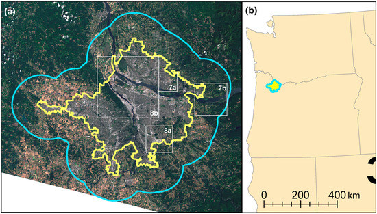
Figure 1.
(a) Combined urban growth boundary (UGB) of the Portland, Oregon and Vancouver, Washington metropolitan areas (yellow line) and nearby rural lands outside the UGB within a 10 km buffer (blue line). Areas examined in Discussion (Figures 7 and 8) are indicated by white boxes. (b) Washington and Oregon states showing the location of the Portland-area UGB. Basemap (a) Landsat 8 red, green, blue (RGB) visual image (LANDSAT_PRODUCT_ID = “LC08_L1TP_046028_20140706_20170305_01_T1”). Basemap (b) state outlines from National Map. Basemap data obtained from U.S. Geological Survey.
To delineate a suitable, nearby, non-urban region of similar area to compare to analysis inside the UGB, we applied a 10 km buffer around the UGB (e.g., as by [50]). This resulted in an outside-UGB area of 2537 km2 compared to an inside-UGB total area of 1437 km2 delineated by the GIS vector outlines. The resulting urban and rural study area encompassed the cities of Portland, Beaverton, Gresham, Hillsboro, and Lake Oswego in Oregon, and Vancouver, Camas, Washougal, and Battleground in Washington State and included all major LC categories. The stark contrast between the urban and rural areas enabled by the historically enforced UGBs provide an ideal testbed to probe the reliability (or uncertainty) of the urban-rural difference framework for assessing SUHIs and the consistency and roles of component LCs in the thermal landscape within and outside a major temperate-zone metropolitan area.
Land cover data for the study were the National Land Cover Database (NLCD 2011), obtained from the U.S. Multi-Resolution Land Characteristics Consortium (MRLC, www.mrlc.gov). The 2011 NLCD products were used as the most recent complete release available. (The 2016 canopy fraction product was not yet available as of the time of this study.) As the NLCD was derived from Landsat data, its native resolution was 30 m pixel size. Of the 20 LC classes present in the NLCD, five were not present in the study area (Perennial Ice/Snow, Dwarf Scrub, Sedge/Herbaceous, Lichens, and Moss). The remaining 15 NLCD LC classes were combined into 10 simpler classes, for which the classification could be more semantically confident given the mixed urban-rural area. The 10 LC classes used were: (1) Open Water, (2) Developed Open Space, (3) Low Intensity Development, (4) Medium Intensity Development, (5) High Intensity Development, (6) Barren Land, (7) Forest (deciduous, evergreen, and mixed combined), (8) Grassland (shrub/scrub, grassland/herbaceous, and pasture/hay combined), (9) Crops, and (10) Wetlands (woody and emergent herbaceous combined). This reclassified LC map was then coarsened to 1 km pixel resolution according to the most abundant component LC class within each 1 km pixel (Figure 2a). This approach follows many other studies, e.g., Sun (2018), who used a 1 km analysis grid to match the resolution of MODIS LST [72]. We also obtained percentage impervious and percentage canopy cover raster data layers from MRLC (2011) and rescaled these to 1 km resolution by the average impervious or canopy fraction within each 1 km pixel (Figure 2c,d).
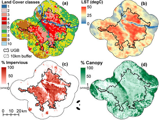
Figure 2.
(a) Dominant LC. Classes in legend are: 1 Open Water, 2 Developed Open Space, 3 Low Intensity Development, 4 Medium Intensity Development, 5 High Intensity Development, 6 Barren Land, 7 Forest, 8 Grassland/Scrub/Pasture, 9 Crops, and 10 Wetlands. (b) Moderate Resolution Imaging Spectroradiometer (MODIS) land surface temperature (LST) in °C. (c) Impervious fraction. (d) Canopy fraction. Black outline is UGB. All maps at 1 km pixel resolution (matching MODIS LST).
LST data from MODIS were used to interrogate SUHI patterns and contrasts, as guided by the recent findings by Phan and Kappas (2018) that MODIS is both highly popular for and highly suitable for SUHI analysis [73]. Although of coarser resolution than Landsat and other sensors, the four-times daily return interval, strong surface temperature fidelity, and readily available post-processed LST data product yield MODIS a practical edge for applications over a variety of city to region to global scales [73]. The Aqua satellite of the MODIS Terra-Aqua pair is thought to pass overhead at a time to record data more similar to the true daily maximum temperatures [73], and so was used in this study. The raster of maximum daily MODIS Aqua LST data for the study area were obtained from Climate Engine (climateengine.org) for the exemplary date 16 August 2012, resulting in a cloud-free, complete data set (Figure 2b). This date was chosen as a representative case study due to its temporal relevance to the 2011 NLCD data and its coincidence with a heatwave, reaching the hottest temperatures of the year (37.8 °C; compared to an annual maximum of 36.7 °C in 2010, 36.1 °C in 2011, and 36.7 °C in 2013) [74]. Because of the Aqua scan angle for this dataset, the nominally 1 km × 1 km square (1 km2) MODIS pixels were actually typically 1 km high × 0.7 km wide (0.7 km2). Due to this difference, the area inside the UGB encompassed 2057 pixels (1440 km2 pixel area) and the area outside the UGB encompassed 3619 pixels (2533 km2 pixel area). This agrees with the outside-UGB area of 2537 km2 and inside-UGB total area of 1437 km2 noted above, with the small differences being due to the difference between raster-based and vector-based area calculations. In this paper, consistent with typical practice, we will still refer to the analysis pixels as nominally of “1 km” resolution, size, or scale.
Analyses were done in ArcMap 10.5 (ESRI, Redlands, CA, USA) and in MATLAB R2017a (Mathworks, Natick, MA, USA). Geographic Information System (GIS) data were handled using projection NAD_1983_UTM_Zone_10N, whether natively or automatically re-projected by ArcMap, and using units of meters or kilometers.
3. Results
3.1. The Surface Urban Thermal Deviation (SUTD) and LST Relations to an UGB
The expected elevation of LST inside the UGB compared to LST outside the UGB was apparent for the Portland–Vancouver metropolitan area. On from the typical hot summer day examined, LST starkly contrasted across the UGB itself (Figure 2b).
We herein define this contrast of urban versus surrounding background temperature, at approximately the whole-city scale, as the “urban thermal deviation” (UTD). The UTD smoothly encompasses the existing “urban heat island” and “urban cool island” concepts, reflecting them as differences in UTD sign. This resolves the previously arbitrary and somewhat illogical separation and semantic confusion between these terms in the literature. The UTD concept is actually a spectrum, spanning from a warmer-than-background city (positive value), to very little urban-rural thermal contrast (UTD near zero), to a cooler-than-background city (negative value).
By example, the Portland–Vancouver metropolitan area exhibited a positive SUTD, on average, during the daytime summer heat wave examined. The median and mean LSTs were higher inside than outside the UGB (Table 1). For the whole study area (Overall, in Table 1, the LST statistics were between those of the inside- and outside-UGB values, but with slightly larger standard deviation. None of the three LST sample populations (inside UGB, outside UGB, overall) were normally distributed (nor did they fit exponential, extreme value, lognormal, or Weibull distributions; Anderson-Darling test, MATLAB R2017a). The median LSTs of each of the three distributions were different (p < 0.05, Wilcoxon rank sum test, MATLAB R2017a). The overall LST population was bimodal, due to its composition as a combination of a left-skewed subpopulation of LST values inside the UGB and a more symmetrical subpopulation of LST values outside the UGB (Figure 3a). LST values ≥44.0 °C in the study area were almost entirely found inside the UGB, whereas values ≤37.0 °C were almost entirely found outside the UGB for the examined summer heatwave.

Table 1.
Descriptive statistics of LST values (°C) with respect to the UGB, difference between the inside and outside UGB median and mean LST values (Overall Surface Urban Thermal Deviation (SUTD)), and descriptive statistics of the whole population of possible pixel-by-pixel SUTD values (°C).
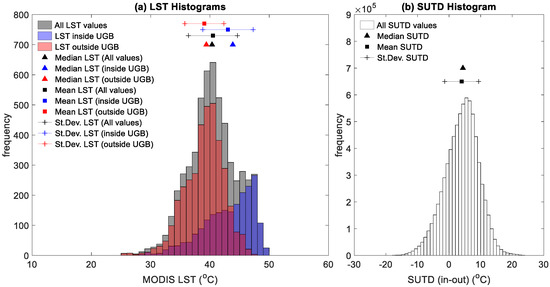
Figure 3.
(a) Comparison of histograms of MODIS LST throughout the study area (gray, n = 5672), inside the UGB (blue, n = 2057), and outside the UGB (red, n = 3615). The overlap of the semi-transparent blue and red histograms may appear purple. For each distribution, the median (triangles) and mean (squares) with one standard deviation error bars are shown by points at top. (b) Histogram of all possible SUTD values, as obtained by subtracting each LST value outside the UGB from each LST value inside (N = 7,436,055). Notice mean and median SUTD are slightly less than the mode, and the SUTD range extends below zero.
Notable, however, was how poorly the mean (43.0 °C) and median (43.9 °C) values of the LST population inside the UGB fit the mode of the data (47 °C), which was a substantially higher LST, near the highest value found anywhere in the study area inside out or outside the UGB (50.0°C). Although the median LST inside the UGB was 4.5 °C greater than the median LST outside the UGB, the mode was a full 7 °C warmer inside the UGB compared to outside (Table 1, Figure 3a). Also, while the UGB appeared to effectively contain hot areas, we observed numerous exceptions where hot areas occurred outside of the UGB (Figure 2b). This highlights the challenge of interpreting SUHI (positive SUTD) urban-rural contrasts with the typical approaches of mean values or buy using a few pixels selected a priori.
An exhaustive population of possible SUTD values was calculated by subtracting each LST value outside the UGB from each LST value inside the UGB. In other words, each of the 3615 pixels outside the UGB was subtracted, in turn, from each of the 2057 pixels inside the UGB, for 3615 x 2057 = 7,436,055 pixel-by-pixel SUTD combinations. This calculated all combinations of possible SUTD values, were one pixel randomly chosen a priori from inside the UGB to be the “urban” end member and one pixel randomly chosen a priori from outside the UGB to be the “rural” end member. The resulting distribution of possible SUTD values was fairly symmetrical, with a median SUTD value of 4.4 °C (Table 1). The mean and median of this SUTD distribution were similar, and also similar to but slightly lower than its mode, which fell in the histogram bin between 6.0–6.9 °C (Figure 3b). The mode of the entire SUTD distribution (5 °C) was 2 °C lower than the difference in the mode of the inside-UGB and outside-UGB LST populations (i.e., 7 °C = mode (LST inside)–mode (LST outside), from Table 1). This again highlights the challenge of interpreting SUHI (positive SUTD) urban–rural contrasts with the typical approaches of mean values or a few selected pixels or stations. In fact, 22% of the possible SUTD values were negative. This means that for 22% of “urban” or “rural” paired points randomly selected a priori, the SUTD is negative and suggests a cooler urban than rural environment overall; the other 78% of random end-member choices give the opposite result, of positive SUTD suggesting a warmer urban than rural environment. Based on random selection of pixels inside vs. outside the UGB, an observer would be about as likely to calculate a SUTD of 0–5 °C as of 5–10 °C (~33% likelihood in each case; Table 2).
Table 2.
Proportion of all possible SUTD values (N = 7,436,055; as in Figure 3b) within 5 °C SUTD bands. Positive values compare a warmer pixel inside the UGB to a cooler pixel outside the UGB (+SUTD, as if representing an urban heat island). Negative values (shaded columns) compare a cooler pixel inside the UGB to a warmer pixel outside the UGB (–SUTD, as if representing an urban cool island).
3.2. LST and SUTD Relations with LC
Analyzing an urban thermal landscape with respect to a formal and enforced UGB, we found that the UGB was as effective at demarcating the spatial division between developed and undeveloped lands as between generally higher urban and lower rural LSTs. The major LC classes inside the UGB were Low Intensity Development (35% of area) and Medium Intensity Development (28% of area). At the 1 km scale analyzed, small developed areas may have been smoothed over, but the major LC classes in the 10 km buffer outside the UGB were Forest (28%), Grassland/Scrub/Pasture (44%), and Crops (16%), with only a few-percent of 1 km pixels dominated by development (Table 3).
Table 3.
Descriptive statistics of subpopulations of LST values within each dominant LC (dominant at 1 km resolution) and inside or outside of the UGB or throughout the study area (Overall). Area % is fraction of spatial area of region covered by that LC, e.g., 3% of area inside UGB was covered by 1 km pixels of dominantly developed open space LC. At right, descriptive statistics of the SUTD within each LC, e.g., the median difference of LST between randomly paired pixels inside and outside the UGB if both pixels were dominated by developed open space was +1.4 °C.
Position inside or outside the UGB did not affect which LCs were warmest or coolest on average, but did affect the absolute values of those LC’s typical LSTs. Both inside and outside the UGB, the warmest LCs were High Intensity Development, Medium Intensity Development, Low Intensity Development, Developed Open Space (e.g., city parks), and Cropland (Table 3 and Figure 4). However, High Intensity Development outside the UGB and Barren Land inside or outside the UGB represented the dominant LC for so few 1 km pixels that further conclusions from these LCs will not be pursued here. Inside the UGB, all the hottest portions of the study area were associated with developed and impervious surfaces, whereas outside the UGB, individual very hot areas were sometimes bare- and dry-looking, tan-colored agricultural fields. In general, the medians of these warm LCs were about 0–3 °C warmer inside the UGB than outside. The absolute hottest LSTs (up to 50.0 °C) in the study area during the examined heatwave were within the generally warm Medium Intensity Development LC.
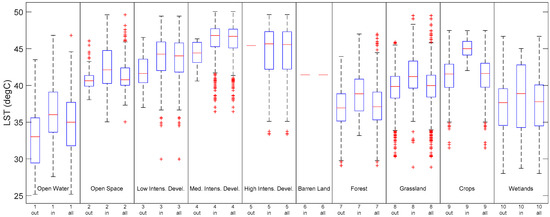
Figure 4.
Comparison of LST by land cover (LC) class inside the UGB, outside the UGB, and overall. Bars are medians, boxes 25th and 75th percentiles (interquartile range, IQR), whiskers extend to 1.5 IQR, and + symbols are outliers. Each group of three plots is for one LC class, as labeled. Lower x-axis labels indicate if plot is based on data from inside UGB, outside UGB, or overall. Note, High Intensity Development outside the UGB and Barren Land inside and outside the UGB were represented by only very small numbers of pixels.
Both inside and outside the UGB, the coolest LCs were Open Water, Forest, and Wetlands. Again, the typical LSTs of each of these LCs differed by position relative to the UGB, with median LSTs of these LCs generally cooler outside the UGB than inside (Table 3), although the interquartile ranges overlapped enough to make practical differences in these typically “cool” LCs perhaps small across the UGB (Figure 4). The absolute coolest pixels (as low as 25.2 °C) were within the generally cool Open Water LC.
We also observed several surprising findings when inspecting the shapes and tails of the LST distributions within these “typically hot” and “typically cool” LCs (Figure 5). Only Forest, Grassland, Crop, and to some extent Wetland LCs resulted in normal, uni-modal, and unskewed LST distributions with fairly balanced and low-frequency tails of coldest and hottest LST values. The merged Grassland LC class exhibited the most positive and negative LST statistical outliers, however (Figure 4).
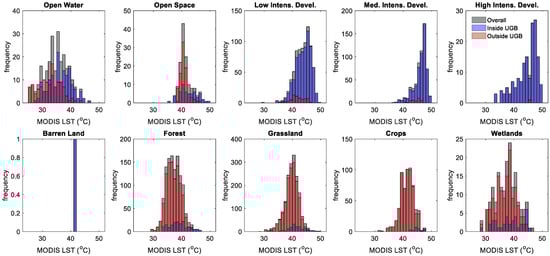
Figure 5.
Comparisons of histograms of LST distributions by LC class for LC pixels occurring inside the UGB (blue), outside the UGB (red), and overall (gray). The overlaps of the semi-transparent blue and red histograms may appear purple. (See Supplement for histograms of % Impervious and % Canopy). Note, High Intensity Development outside the UGB and Barren Land inside and outside the UGB were represented by only very small numbers of pixels.
High, Medium, and Low Intensity Development LST distributions were largely uni-modal but strongly right-skewed, such that their mean LSTs were not good representations of their higher medians and modes (Figure 5). The peaks of the High and Medium Intensity Development LSTs fell between 40–45 °C, with Low Intensity Development LSTs spread between about 38–44 °C. All three types of intense development had their left-skewed tails extend near or to 30 °C LST lows. After Grassland, Medium Intensity Development exhibited the most cool LST statistical outliers, all outside the UGB (Figure 4). In contrast to the other developed LCs, the Developed Open Space LST distribution was more right-skewed, such that its mean LST was not a good representation of its lower median and mode (Figure 5). The Open Space LST peak was between 30–35 °C, with very few cooler values but with sizable weight in the right-tail of LST values from 35–45 °C. After Grassland, Developed Open Space exhibited the most warm LST statistical outliers, all inside the UGB (Figure 4). There were too few 1 km pixels dominated by Barren Land to yield a useful distribution with 1 °C histogram bins (Figure 5). Histograms like Figure 5, but for the distribution of impervious area (Figure S1) and canopy cover (Figure S2) are available in the online supplement.
The observed within-LC temperature variations were not entirely predictably correlated with impervious area fraction, as was expected, however, nor with canopy area fraction. Overall, the relationship (linear regression) of LST with impervious cover >0% was positive, with LST increasing with increasing impervious fraction regardless of being located inside or outside the UGB (Figure 6a–c). However, inside the UGB some of the highest and lowest LST values each occurred in the same 1 km areas as both the highest and lowest average impervious fractions (Figure 6a), i.e., some very warm areas had very low impervious fractions, and vice versa.
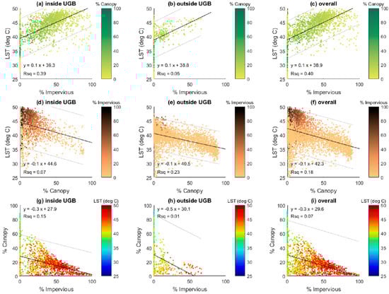
Figure 6.
Scatterplots of relations among LST, percent impervious area, and percent canopy area, inside the UGB (a,d,g), outside the UGB (b,e,h), and overall (c,f,i). Lines of best fit in black and equations, 95% prediction intervals in gray.
As expected, the overall relationship of LST with canopy cover was negative, with LST decreasing with increasing canopy fraction regardless of being located inside or outside the UGB (Figure 6d–f), but again with substantial scatter around this tendency. The data exhibited smaller residuals around a linear regression outside the UGB, compared to inside, i.e., the linear model of LST with canopy fraction was more representative outside the UGB. This relationship broke down, however, for canopy fractions below about 10%, where LST took on a full range of low (~25 °C) to high (~50 °C) values. In fact, the greatest abundance of low LST values within any decile of canopy fraction clustered at canopy fractions <10%. The scatter of various LST values was further illustrated when examining the tradeoff in area fraction between impervious and canopy cover (Figure 6g–i).
4. Discussion
The aim of this study was to examine the relation of urban temperatures to an urban growth boundary, the composition of the city’s elevated temperatures in relation to constituent LCs, and the sentinel and sometimes counter-intuitive variations in LST within LCs in and around a city. To date, the nomenclature of the atmospheric “urban heat island” (UHI) and surface temperature “surface urban heat island” (SUHI) has provided a simple framework to interrogate how urban and rural areas differ in their thermal conditions. Studies that illustrate these differences span decades, yet, as we begin to examine the implications of our development and urbanization processes in relation to a warming climate, we argue that science and society need more precise and accurate nomenclature. The most compelling case for this argument is that fact that the original formulation of the (S)UHI concept was inadvertently biased by a perspective of an urban area in a surrounding densely vegetated, humid agro- or natural-ecosystem, typically of a temperate region; many recent studies have shown that, in drier and less vegetated regions, urban areas sometimes act as large “urban cool islands” instead [40]. Replacing the (S)UHI vs. (S)UCI dipole with instead a more nuanced concept of an “urban thermal deviation” of urban temperatures compared to background temperatures provides a fresh framework within which to seamlessly embrace UHI and UCI poles across a (S)UTD spectrum from positive (heat island-like), through zero (thermally comparable to background), to negative (cool island-like) values. This updated framework may help analysis begin to focus on the magnitudes of the urban vs. rural thermal contrasts as much as the signs. Also, by explicitly including a zero value within the (S)UTD spectrum, which was implicit but absent in the traditional dipole approach, the (S)UTD framework may enable compelling new research questions. For example: What would it take to reduce a positive UTD to zero, seamlessly blending the urban thermal environment with its surroundings?
Perhaps the most important, yet underappreciated, issue regarding all these nuances of calculating SUTD (or SUHI, UHI, SUCI, UCI, etc.) values is the socio-economic and racial equity dimensions of our practices to date for choosing “representative” urban and rural temperature end-members. If a large number of weather stations were averaged, but their locations were accidentally skewed toward greener and cooler areas of the city, perhaps where more affluent homeowners establish online personal weather stations, then one might find highly skewed results about the difference between urban and rural areas that underestimates the heat stress of less green, less affluent neighborhoods. If, for example, a city has a small urban core and extensive lower density residential development within city limits, should the urban end-member temperature be in the residential or downtown areas? Even if one took an area-weighted average of the two, would that be “representative”? A growing body of literature is showing that urban greenery and related urban heat mitigation are systematically more available to more affluent residents, whereas lower-income neighborhoods frequently have lower canopy cover and higher local temperatures [11,14,26,75,76,77]. This raises the question, then, not only of how to choose an “urban” end member to be representative of the urban landscape, but also what is “representative—and for whom?” To tackle the important social and environmental justice angle of urban warming and its inequity, we first need more clear and precise language to describe different scales and magnitudes of warming or cooling. We then also need to develop a practice of more thoroughly interrogating the range of possible urban heat island or urban cool island experiences urban, peri-urban, and rural residents may experience, rather than leaning on fairly blunt, single-valued metrics such as (S)UHI. Moving beyond single-valued metrics may be a useful step toward expanding our perception and study of urban versus rural thermal equity.
The SUTD framework of this study takes a step further than the urban thermal variability reflected in prior studies of one-dimensional transects across a city (e.g., [48]), to now reflect the full variability of temperatures across a city and compared to its surroundings. Beyond transects, the SUTD framework encourages examining both LST and SUTD as histograms (e.g., Figure 3 and Figure 5) and taking increased care to interrogate the meaning and representativeness of statistics such as LST and SUTD mean, median, or mode. Our findings, from testing the SUTD approach for an example city, suggest there is added value in characterizing the spatial variations in urban heat and coolness with greater statistical detail than has been possible, to date, using the prevalent, single-valued SUHI (or SUCI) metric and the binary SUHI versus SUCI conceptual framework. Moving toward more spatially exhaustive, statistical representations of urban heat, cool, or urban-rural thermal difference is quite easily achievable, especially for studies using increasingly abundant remote sensing data. Adopting, and using nomenclature to match, a view that (S)UHI and S(UCI) values exist on a (S)UTD spectrum from cool-to-zero-to-warm contrasts between urban and rural environments may provide a more accurate notion of both the relative thermal position and always-changing nature of the urban thermal environment. These two approaches, more spatially-exhaustive analysis and contextualization of urban/rural temperature contrast on a (S)UTD continuum, may together provide more nuanced and actionable information of scientific and societal value, compared to comparing “urban” or “rural” dipoles selected a priori and of uncertain representativeness.
The results of this study also suggest that a single SUHI value is unlikely to be usefully representative of the urban thermal anomaly relative to the background rural landscape. Temperatures can be highly variable among (Figure 4), and highly skewed within (Figure 5), different LCs. Even if a “representative” LC class could be identified for an urban or rural setting, an accidentally anomalous choice of end-member location that is notably warmer or cooler than is typical for that LC is reasonably statistically probable given the long tails on some LC’s LST distributions (Figure 5). This may result in reported SUHI values in the literature to date often, but unknowingly and randomly, underestimating (or overestimating) urban warming. Such effects can be especially misleading if a SUHI calculation is based on few points in the urban and rural areas, or even if the SUHI calculation is based on spatially exhaustive data (such as remotely sensed data) but mean values are used. Our results demonstrated that medians would generally be better choices than means (Figure 3b), but either may be several degrees higher or lower than the mode of a given LC’s temperature, which might arguably be the most representative. Statistical tests may also help identify if a suspected relationship between temperature and LC is random, underestimated or overestimated.
4.1. Toward More Precise Descriptions of Variations in Urban Temperatures
4.1.1. From Heat (or Cool) Islands to the Urban Thermal Deviation (UTD)
To improve our ability to describe the variation in urban temperatures and so to study them effectively and seek to manage them equitably and efficiently, we propose three revisions to the confusing prevalent terminology around temperature variation in and around urban areas. In our first description, we define the contrast of urban temperature versus surrounding background temperature, at approximately the whole-city scale, as the “urban thermal deviation” (UTD). The UTD is essentially the combination the existing “urban heat island” and “urban cool island” concepts, which have been separated to date despite being two sides of the same phenomenon. Within the (S)UTD concept, the deviation of the urban temperature from the rural thermal background lies on a spectrum from positive (S)UTD (city warmer than background), to very little (UTD near zero), to negative (S)UTD (cooler city).
From a science and management perspective, a transition from (S)UHI and (S)UCI to the combined (S)UTD spectrum may help better represent how myriad urbanization processes (e.g., expansion, densification, watering status, etc.) can—and do—change over time both as sudden step-changes and as gradual shifts along an urban thermal spectrum. The concept of urban heat as a spectrum from cooler-to-equivalent-to-warmer conditions from the background might prove encouraging in setting management goals. For example, in the binary concept of a city presenting a UHI compared to a cooler background (or vice versa, and mainly as a function of its accidental fate to reside in a particular biome [35,48]), it might be difficult to recognize progress in cooling the city, e.g., by careful urban planning and resident action, as the city may still remain substantially warmer than its surroundings. Using the (S)UTD spectrum concept, however, a city might recognize its progress moving from a warmer position on the spectrum toward a more desirable value closer to zero, celebrate progress, and realistically motivate further progress.
4.1.2. Distinguishing Urban Microthermal Extremes (MTEs)
As at the city scale, making significant progress on the science and management of a warm (or cool) (S)UTD will also require improvement in understanding of neighborhood-by-neighborhood and block-by-block contributions to warming. Unfortunately, intra-urban variations in temperature have suffered to date in the literature from semantic conflation with city-scale terms. For example, an “urban cool island” has variously been used to describe a city that seems cooler than its surroundings on average (e.g., [40,48,49,50,51,78]), but also to describe a green park, at a much finer spatial scale, within an otherwise warm development (e.g., [26,40,53,56,63,79,80,81,82]). Further, while “cool island” may be used to describe an urban park’s effect, the same phenomenon but of opposite sign, e.g., of a warm commercial area within an otherwise cooler low intensity development area, is more typically called a “hot spot” (e.g., [83]) rather than using parallel language. Finally, the usage of “park cool island” and “hot spot” in the literature has been vague as to if the neighborhood surrounding these foci must be of starkly different temperature (e.g., hot around a cool park, or quite cool around a hot spot), of merely contrasting temperature (e.g., moderate around a cool park, or warm around an exceptionally hot spot), or of opposite expected temperature (e.g., cool when expected to be hot according to its LC, or vice versa).
To resolve these semantic confusions around thermal contrasts at the intra-city scale, we first define an urban “micro-thermal extreme” (MTE) as a discrete area the temperature of which is significantly more extreme than its land cover would suggest. In other words, an MTE is an intra-city thermal variation of an expected, but extreme and notable, nature. For example, an exceptionally hot industrial area within a generally warm industrial zone would be a hot MTE. An exceptionally cold tree stand within a generally cool vegetated area would be a cold MTE.
In this study, although some LCs exhibited an overall tendency to be warmer and others cooler, as expected, we did find discrete areas of ‘typically warm’ LCs that exhibited exceptionally hot temperatures, and discrete areas of ‘typically cool’ LCs that exhibited exceptionally cold temperatures. An example of a hot MTE was present within the study area among some Medium and High Intensity Development in Vancouver, WA; here, ten of the hottest pixels of the study area occurred adjacent to each other (Figure 7a). More broadly throughout the study area, of the 26 hottest pixels in the entire metropolitan landscape (>49 °C LST), six were dominated by High Intensity Development, 16 by Medium Intensity Development, two by Grassland/Scrub/Pasture, one by Low Intensity Development, and one by Developed Open Space. Note, the threshold over which an area is considered a hot MTE will vary by study, by location, day, and example; in this study 49 °C was used as it provided a threshold exceeded by only about 0.5% of pixels within the examined data. In this study, hot MTEs typically had high impervious and low canopy fractions.

Figure 7.
Examples of urban micro-thermal extremes (MTEs); locations shown in the Figure 1 city map. (a) Hot MTEs: Exceptionally hot, discrete areas of typically warm/moderate-temperature LC or surroundings. (b) Cold MTEs: Exceptionally cold, discrete areas of typically cool/moderate-temperature LC or surroundings. (LC classes are: 1 Open Water, 2 Developed Open Space, 3 Low Intensity Development, 4 Medium Intensity Development, 5 High Intensity Development, 6 Barren Land, 7 Forest, 8 Grassland/Scrub/Pasture, 9 Crops, and 10 Wetlands.)
Cold MTEs in the study area typically occurred over water features in the Portland–Vancouver metropolitan landscape. Even excluding open water LC, the banks, islands, and wetlands of the Columbia River still exhibited the coolest spots in the area during the examined heat wave (Figure 7b), accounting for 25 of the 28 coolest, non-water pixels. The narrower and more urbanized banks of the Willamette River did not exhibit the same cold MTE effect as the wide Columbia River. Of the 28 coolest, non-water pixels (<31 °C LST), nine were dominated by Wetland LC, ten by Grassland/Scrub/Pasture, eight by Forest, and one by Low Intensity Development. Interestingly, three of the eight exceptionally cool forest pixels provided the only cold MTE locations not occurring near the Columbia River. One of these points occurred adjacent to a large reservoir outside the UGB (Henry Haag Lake). The other two occurred in a patch of apparently dense (possibly un-logged), private forest land west of Gales Creek, Oregon. The one cold MTE detected within Low Intensity Development occurred on the eastern shore of the large and shallow Lake Vancouver, in Vancouver, WA. The remainder of the cold MTE lands in the study area were along the Columbia River banks. An additional 54 water LC pixels, all within the Columbia River or Vancouver Lake, were also exceptionally cool (<31 °C LST). Note, the threshold below which an area is considered a cold MTE will vary by study, by biome, climate, day, and example, as for the hot MTE threshold.
4.1.3. Distinguishing Urban Microthermal Anomalies (MTAs)
In addition to observing that the temperatures of some areas within the metropolitan and peri-urban region were in the expected direction but even more extreme than would have been predicted from the LC or surroundings (i.e., MTEs), we observed the opposite as well: specific areas within the region that exhibited temperatures opposite what would have been predicted from the LC or surroundings. To name and capture this phenomenon we define an urban “micro-thermal anomaly” (MTA) as a discrete area that exhibits temperatures opposite the typical expectation for its LC or surroundings. For example, a significantly cool park area within a typically warm, highly developed LC patch would be a cool MTA. Previously, this phenomenon may have been called an urban park “cool island,” but this is too easily confused with use of the term “cool island” to describe whole irrigated cities in dryland areas (i.e., UCI). Similarly, a significantly warm area such as a power transmission station within a densely forested park would be a warm MTA. Previously, this phenomenon may have been called a “hot spot,” but this language has been imprecise as it does not distinguish between notable, anomalous warm areas which would typically be cool (warm MTA) and hotter-than-usual areas of a typically warm LC (hot MTE).
In the Portland–Vancouver area during the examined summer heatwave we did observe important exceptions to the general tendency of some LCs to be cooler and others warmer, where individual pixels or small clusters of pixels exhibited the opposite LST signature. These exceptions are especially important because they may be indicators of either cooling solutions in otherwise typically warm LC areas or, conversely, of problematically warm areas that may cause heat and drought stress more than the surrounding typically-cool LC classification might suggest. An example of a warm MTA occurred in an area of High Intensity Development mixed with Forest LC (Figure 8a). This and other warm MTAs occurred in the study area among Open Water, Forest, or Wetland LC that would be expected to be typically cool but exhibited, instead, LST > 44 °C.
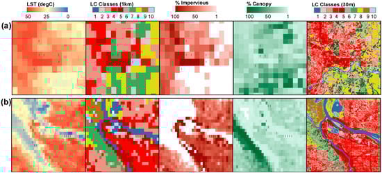
Figure 8.
Examples of urban micro-thermal anomalies (MTAs); locations shown in the Figure 1 city map. (a) Warm MTAs: Starkly warm, discrete areas of typically cool LC or surroundings. (b) Cool MTAs: Starkly cool, discrete areas of typically warm LC or surroundings. (LC classes are: 1 Open Water, 2 Developed Open Space, 3 Low Intensity Development, 4 Medium Intensity Development, 5 High Intensity Development, 6 Barren Land, 7 Forest, 8 Grassland/Scrub/Pasture, 9 Crops, and 10 Wetlands.)
For the example warm MTA illustrated in Figure 8a, both the scale and intensity of hot- and cool-LC juxtapositions likely played a role in producing this result, as did the resolution of the data analyzed. Despite the prominent forested parks in the area, the great intensity of impervious area and LC juxtaposition and mixing below the resolution of the analysis permitted LST values to be elevated, even in the locations of the “typically cool,” dominantly Forest LC pixels. This subgrid effect likely explains the four more northern points of interest in Figure 8a (upper four black dots). At a 30 m native NLCD scale, these points were located on the boundaries between forested and intensely developed LCs (right-most panel, Figure 8a), but at the 1 km scale the locations were dominated by forest area. Their expression as warm MTAs are therefore likely due to the heat from the intensely developed lands overwhelming, at subgrid scale, the coolness of the spatially slightly more abundant forest area.
The southern two points of interest in this same neighborhood (lower two black dots, Figure 8a) exhibited a slightly different phenomenon leading to warm MTA conditions, however. These two points were classified as Forest or Wetland at the 1 km scale, and yet still exhibited highly elevated LST during a heatwave, >44°C. (Note, the temperature threshold or contrast from background for which an area is considered a warm MTA will vary by study, by biome, climate, day, and example.) In contrast to the more northern warm MTA forested points, though, these two more southern points were well-surrounded by Water and Wetland (blue), Forest (dark green), and Grassland/Scrub/Pasture (yellow). The prior explanation of their warm MTA status being conveyed due to abundant heat form a sub-dominant LC at subgrid scale does not hold, therefore. In this case, it may be more likely that true anomalies of surface energy balance, or aerodynamic and biophysical effects of heat “spill-over” from nearby (but not immediately adjacent) intensely developed areas, were the key governing factors. These same factors may also have played a role in the elevated temperatures of the more northern four points, but it is more difficult to surmise from the available information.
Examples of cool MTAs in the Portland–Vancouver area also occurred during the examined heatwave, where typically warm LC such as High, Medium, or Low Intensity Development exhibited surprisingly low LST values (e.g., <37 °C). Prominent areas of cool MTAs clustered: (i) among the High Intensity Development in northwest Portland between the large greenspace of Forest Park and the adjacent Willamette River, (ii) among the Medium-to-High Intensity Development of northern Portland between the airport and Hayden Island on the shores of the Columbia River, and (iii) among the mixed Low-Medium Intensity Development of Vancouver on the eastern shore of Vancouver Lake (Figure 8b). These areas all had in common their placement of intense development next to a large waterbody. As with the warm MTA occurrences discussed above, is likely that these apparent cool MTA occurrences reflect a combination of apparent cooling due to sub-grid mixing within the 1 km pixels and actually cooler biophysical processes and surface energy balance outcomes on the ground.
The seven eastern points of interest in Figure 8b (five points in a row toward the right of the figure, one point nearby to their northwest, and one point more inland from the lake near the top of the figure) we interpret as more likely arising from the latter explanation, actual less-than-expected longwave radiation due to aerodynamic or biophysical effects on the surface energy balance. These points are well surrounded by intense development that would otherwise be typically warm, are set-back from direct shoreline exposure, and so must have a compensatory cooling process in effect. These seven locations would be ideal candidates to investigate further with ground-based research measurements, to determine more specifically what is supporting their desirable, apparently cooler, conditions.
In contrast, the nine western points of interest in Figure 8b (nine black dots more to the left sides of the panels), may include some of the same real aerodynamic or biophysical cooling effects, but we interpret as perhaps being dominated by subgrid mixed-pixel effects. Although intense development covered a majority of the 1 km pixel, it is possible that forest or water LC was only slightly less extensive, and quite cool, skewing the overall apparent LST at the 1 km scale. However, even if this is the case, it bears noting that a similar situation occurred among the warm MTA examples of Figure 8a, but in those warm MTA cases the slight majority of area covered by forest or water LC was not able to overcome the subgrid warmth provided by the minority intense development. In this situation of cool MTAs, the opposite seems to be occurring, where a slight minority of area covered by forest or water LC was able to overcome the subgrid warmth provided by majority intense development. Therefore, although the identification of these MTA may include artifacts from subgrid scales, there is still something to be learned from why some locations on the landscape show up as warm MTAs but other similar ones as cool MTAs; this might be a useful subject of future research.
Although not perhaps surprising that large cool waterbodies may provide a cooling ecosystem service to adjacent more typically warm LCs as shown by these cool MTAs, this highlight should not be overlooked as a tool of potential use to urban planners. For example, typically warm High Intensity Development could be intentionally planned for shorelines to maximize the cooling service of adjacent large water bodies; of course, this might also prove contentious. Building a public greenway park along the shores of a large, cool waterbody might meet with more vocal approval and be intended to provide riparian habitat value and physical and mental health opportunities (although not necessarily equitably [15,76,84,85]). However, the insight of cool MTAs located on shorelines at least inspires new compelling questions: Is placing a green LC, that would typically already be cool, in the location of maximum cooling service from the waterbody the most efficient way to mitigate overall urban heat? And for whom? As many cities worldwide are found on river, lake, or ocean shorelines [86], this topic of urban design relative to the natural cooling services of the waterbodies warrants further research to determine biophysical, environmental, and social tradeoffs and consequences for urban ecology and resident equity, particularly amid ongoing broader trends of urbanization and climate change. In sum, we find that it may be useful in guiding more nuanced appreciation of relations between SUTD and LC and urban planning to pay attention to occurrences of MTAs, distinguish them from MTEs, and interrogate whether MTAs arise from actual biophysical contrasts in urban surface energy and water balances, from subgrid effects of resolution of analysis, or perhaps a combination of both, as they are not mutually exclusive possibilities; this is an area of ongoing development in the research field.
5. Conclusions
The field of urban climate studies is rapidly expanding with new assessments, techniques, and applications. While a large proportion of these studies rely on LST to characterize variations in urban temperatures, only few challenge long-held presumptions about surface urban heat islands (SUHIs). It is becoming apparent that the long-standing, dominant (S)UHI nomenclature, and the presumption that cities are typically warmer than their surroundings, is actually a historical artifact of a temperate-zone/humid-zone sampling bias of much of the work in this field. Recent evidence from cities in the Middle East, southwest US, and other dryland areas indicate that urban areas can also be consistently cooler than adjacent rural areas [40]. However, the resulting addition of “urban cool islands” to the literature has only enabled partial progress toward resolving this bias, as it has moved a monolithic UHI field into a still too simplistic binary UHI/UCI framework. In fact, the difference between urban and background temperature must fall across a continuum from negative (cooler city) to positive (warmer city) values, also be inclusive of a hypothetical zero-difference value. In this study we advance the spanning concept of the “urban thermal deviation” (UTD or SUTD) to encompass this continuum of urban/rural temperature contrasts and expand the UHI/UCI binary to a spectrum. Further, we demonstrate and encourage further interrogation of single-valued metrics of urban/rural thermal contrast, and especially of the representativeness of the urban and rural end-members that must be chosen a priori for such calculations. In addition to asking “Representative of what?”, i.e., how statistically representative are the chosen end-members of the urban landscape, really? We also encourage future research to ask “Representative for whom?”, being conscious that LCs, urban canopy, urban temperatures, and micrometeorological infrastructure [31] are not typically equitably distributed among city residents [11,14,26,75,76,77].
In this study we developed and demonstrated this updated framework for understanding urban/rural contrasts in temperature as a SUTD spectrum, aided by evidence from a discrete case of a metropolitan area with a well-established urban growth boundary. Comparing urban and rural pixels across this well-demarcated boundary, we found that the SUTD is better understood as a distribution of a whole population of possible urban/rural LST contrasts, rather than any random urban/rural pairing, or even mean or median SUTD values (Figure 3b). In fact, we surmise that most SUHI and SUCI values reported to date, if based on a difference between mean (or even median) temperature values within the chosen urban and rural end-members as is typical, are at best indicative, not representative, and at worst, misleading as to the characteristic urban and rural temperatures and their contrast.
At the finer spatial scale of LC patches within a city, it is well-appreciated that major exceptions to background urban and rural temperatures exist and are important and useful to understand, such as cool parks inside a city and hot dry fields outside a city. A useful distinction that has been lacking to date, however, is whether local thermal exceptions are what we term (a) microthermal extremes (MTEs), which tend in the same direction (warm or cool) as their LC or surroundings but to extreme values, or (b) true microthermal anomalies (MTAs), which run counter to expectations for their LC or surroundings. The distinction is important because the former, MTEs, suggests a need for moderation in the thermal landscape, whereas the latter, MTAs, may suggest possible solutions.
In sum, the novel study of a metropolitan setting with a historically enforced urban growth boundary has provided insight into the utility of a UGB for controlling the sprawl of both urban development and its associated thermal signature into the rural surrounds. It has also inspired the suggestion of more inclusive terminology aimed toward escaping strictures of past semantically conflated or binary heat/cool island frameworks to more general urban thermal deviations. We submit that the (S)UTD framework, in addition to being more inclusive, may be a more hopeful framework for considering urban thermal conditions. As the (S)UTD spectrum naturally includes the zero-point, where urban temperature would be equivalent to the background biome, it is the first framework, to our knowledge, to suggest an environment-neutral target for urban thermal management. Arguably, working toward SUTD = 0 may be an important and useful goal for urban sustainability in the age of climate change. Under conditions of rising heat-related urban mortality due to both densification and climate change, it is more important and urgent than ever to understand and characterize just how hot a city is, for comparison to surrounding areas, other cities, and other times in the past or future.
Supplementary Materials
The following are available online at https://www.mdpi.com/2072-4292/11/22/2683/s1, Figure S1: Comparisons of histograms of % Impervious distributions by LC class for LC pixels occurring inside the UGB, outside the UGB, and overall. Figure S2: Comparisons of histograms of % Canopy distributions by LC class for LC pixels occurring inside the UGB, outside the UGB, and overall.
Author Contributions
Conceptualization, K.B.M., V.S.; methodology, K.B.M.; investigation, Y.M.; final analysis, K.B.M.; data curation, Y.M.; original draft preparation, K.B.M., Y.M., V.S.; writing review and editing, K.B.M.; visualization, K.B.M., Y.M.; funding acquisition, K.B.M., V.S.
Funding
This material is based upon work supported by the National Science Foundation CAREER and Hydrological Sciences programs under Grant No. 1751377 to K.B.M. Moffett at Washington State University.
Conflicts of Interest
The authors declare no conflict of interest.
References
- Basu, R. High ambient temperature and mortality: A review of epidemiologic studies from 2001 to 2008. Environ. Health 2009, 8, 40. [Google Scholar] [CrossRef] [PubMed]
- Gabriel, K.M.A.; Endlicher, W.R. Urban and rural mortality rates during heat waves in Berlin and Brandenburg, Germany. Environ. Pollut. 2011, 159, 2044–2050. [Google Scholar] [CrossRef] [PubMed]
- Li, Y.; Ren, T.; Kinney, P.L.; Joyner, A.; Zhang, W. Projecting future climate change impacts on heat-related mortality in large urban areas in China. Environ. Res. 2018, 163, 171–185. [Google Scholar] [CrossRef] [PubMed]
- Lowe, S.A. An energy and mortality impact assessment of the urban heat island in the US. Environ. Impact Assess. Rev. 2016, 56, 139–144. [Google Scholar] [CrossRef]
- Paravantis, J.; Santamouris, M.; Cartalis, C.; Efthymiou, C.; Kontoulis, N. Mortality Associated with High Ambient Temperatures, Heatwaves, and the Urban Heat Island in Athens, Greece. Sustainability 2017, 9, 606. [Google Scholar] [CrossRef]
- Petkova, E.; Horton, R.; Bader, D.; Kinney, P. Projected Heat-Related Mortality in the U.S. Urban Northeast. Int. J. Environ. Res. Public. Health 2013, 10, 6734–6747. [Google Scholar] [CrossRef]
- Smargiassi, A.; Goldberg, M.S.; Plante, C.; Fournier, M.; Baudouin, Y.; Kosatsky, T. Variation of daily warm season mortality as a function of micro-urban heat islands. J. Epidemiol. Community Health 2009, 63, 659–664. [Google Scholar] [CrossRef]
- Son, J.Y.; Lane, K.J.; Lee, J.T.; Bell, M.L. Urban vegetation and heat-related mortality in Seoul, Korea. Environ. Res. 2016, 151, 728–733. [Google Scholar] [CrossRef]
- Wang, D.; Lau, K.K.L.; Ren, C.; Goggins, W.B.I.; Shi, Y.; Ho, H.C.; Lee, T.C.; Lee, L.S.; Woo, J.; Ng, E. The impact of extremely hot weather events on all-cause mortality in a highly urbanized and densely populated subtropical city: A 10-year time-series study (2006–2015). Sci. Total Environ. 2019, 690, 923–931. [Google Scholar] [CrossRef]
- Johnson, D.P.; Wilson, J.S. The socio-spatial dynamics of extreme urban heat events: The case of heat-related deaths in Philadelphia. Appl. Geogr. 2009, 29, 419–434. [Google Scholar] [CrossRef]
- Voelkel, J.; Hellman, D.; Sakuma, R.; Shandas, V. Assessing Vulnerability to Urban Heat: A Study of Disproportionate Heat Exposure and Access to Refuge by Socio-Demographic Status in Portland, Oregon. Int. J. Environ. Res. Public. Health 2018, 15, 640. [Google Scholar] [CrossRef] [PubMed]
- Huang, G.; Zhou, W.; Cadenasso, M.L. Is everyone hot in the city? Spatial pattern of land surface temperatures, land cover and neighborhood socioeconomic characteristics in Baltimore, MD. J. Environ. Manag. 2011, 92, 1753–1759. [Google Scholar] [CrossRef] [PubMed]
- Wang, J.; Kuffer, M.; Sliuzas, R.; Kohli, D. The exposure of slums to high temperature: Morphology-based local scale thermal patterns. Sci. Total Environ. 2019, 650, 1805–1817. [Google Scholar] [CrossRef] [PubMed]
- Jenerette, G.D.; Miller, G.; Buyantuev, A.; Pataki, D.E.; Gillespie, T.W.; Pincetl, S. Urban vegetation and income segregation in drylands: A synthesis of seven metropolitan regions in the southwestern United States. Environ. Res. Lett. 2013, 8, 044001. [Google Scholar] [CrossRef]
- Jenerette, G.D.; Harlan, S.L.; Stefanov, W.L.; Martin, C.A. Ecosystem services and urban heat riskscape moderation: Water, green spaces, and social inequality in Phoenix, USA. Ecol. Appl. 2011, 21, 2637–2651. [Google Scholar] [CrossRef]
- Aflaki, A.; Mirnezhad, M.; Ghaffarianhoseini, A.; Ghaffarianhoseini, A.; Omrany, H.; Wang, Z.H.; Akbari, H. Urban heat island mitigation strategies: A state-of-the-art review on Kuala Lumpur, Singapore and Hong Kong. Cities 2016, 62, 131–145. [Google Scholar] [CrossRef]
- Wang, Y.; Berardi, U.; Akbari, H. Comparing the effects of urban heat island mitigation strategies for Toronto, Canada. Energy Build. 2016, 114, 2–19. [Google Scholar] [CrossRef]
- Wang, Y.; Akbari, H. Analysis of urban heat island phenomenon and mitigation solutions evaluation for Montreal. Sustain. Cities Soc. 2016, 26, 438–446. [Google Scholar] [CrossRef]
- Zhou, W.; Huang, G.; Cadenasso, M.L. Does spatial configuration matter? Understanding the effects of land cover pattern on land surface temperature in urban landscapes. Landsc. Urban Plan. 2011, 102, 54–63. [Google Scholar] [CrossRef]
- Villanueva-Solis, J. Urban Heat Island Mitigation and Urban Planning: The Case of the Mexicali, B. C. Mexico. Am. J. Clim. Chang. 2017, 06, 22–39. [Google Scholar] [CrossRef][Green Version]
- Shandas, V.; Voelkel, J.; Williams, J.; Hoffman, J. Integrating Satellite and Ground Measurements for Predicting Locations of Extreme Urban Heat. Climate 2019, 7, 5. [Google Scholar] [CrossRef]
- Oke, T.R. City size and the urban heat island. Atmos. Environ. 1967 1973, 7, 769–779. [Google Scholar] [CrossRef]
- Arnfield, A.J. Two decades of urban climate research: A review of turbulence, exchanges of energy and water, and the urban heat island. Int. J. Climatol. 2003, 23, 1–26. [Google Scholar] [CrossRef]
- Tran, H.; Uchihama, D.; Ochi, S.; Yasuoka, Y. Assessment with satellite data of the urban heat island effects in Asian mega cities. Int. J. Appl. Earth Obs. Geoinf. 2006, 8, 34–48. [Google Scholar] [CrossRef]
- Lee, H.; Mayer, H.; Chen, L. Contribution of trees and grasslands to the mitigation of human heat stress in a residential district of Freiburg, Southwest Germany. Landsc. Urban Plan. 2016, 148, 37–50. [Google Scholar] [CrossRef]
- Declet-Barreto, J.; Brazel, A.J.; Martin, C.A.; Chow, W.T.L.; Harlan, S.L. Creating the park cool island in an inner-city neighborhood: Heat mitigation strategy for Phoenix, AZ. Urban Ecosyst. 2013, 16, 617–635. [Google Scholar] [CrossRef]
- Ferwati, S.; Skelhorn, C.; Shandas, V.; Makido, Y. A Comparison of Neighborhood-Scale Interventions to Alleviate Urban Heat in Doha, Qatar. Sustainability 2019, 11, 730. [Google Scholar] [CrossRef]
- Voelkel, J.; Shandas, V. Towards Systematic Prediction of Urban Heat Islands: Grounding Measurements, Assessing Modeling Techniques. Climate 2017, 5, 41. [Google Scholar] [CrossRef]
- Oke, T.R. The energetic basis of the urban heat island. Q. J. R. Meteorol. Soc. 1982, 108, 1–24. [Google Scholar] [CrossRef]
- Oke, T.R.; Johnson, G.T.; Steyn, D.G.; Watson, I.D. Simulation of surface urban heat islands under ‘ideal’conditions at night Part 2: Diagnosis of causation. Bound. Layer Meteorol. 1991, 56, 339–358. [Google Scholar] [CrossRef]
- Peterson, T.C. Assessment of Urban Versus Rural in Situ Surface Temperatures in the Contiguous United States: No Difference Found. J. Clim. 2003, 16, 2941–2959. [Google Scholar] [CrossRef]
- Martin-Vide, J.; Sarricolea, P.; Moreno-García, M.C. On the definition of urban heat island intensity: The “rural” reference. Front. Earth Sci. 2015, 3. [Google Scholar] [CrossRef]
- Gaffin, S.R.; Rosenzweig, C.; Khanbilvardi, R.; Parshall, L.; Mahani, S.; Glickman, H.; Goldberg, R.; Blake, R.; Slosberg, R.B.; Hillel, D. Variations in New York city’s urban heat island strength over time and space. Theor. Appl. Climatol. 2008, 94, 1–11. [Google Scholar] [CrossRef]
- Wang, F.; Ge, Q.; Wang, S.; Li, Q.; Jones, P.D. A New Estimation of Urbanization’s Contribution to the Warming Trend in China. J. Clim. 2015, 28, 8923–8938. [Google Scholar] [CrossRef]
- Zhao, L.; Lee, X.; Smith, R.B.; Oleson, K. Strong contributions of local background climate to urban heat islands. Nature 2014, 511, 216–219. [Google Scholar] [CrossRef]
- Deilami, K.; Kamruzzaman, M.; Liu, Y. Urban heat island effect: A systematic review of spatio-temporal factors, data, methods, and mitigation measures. Int. J. Appl. Earth Obs. Geoinf. 2018, 67, 30–42. [Google Scholar] [CrossRef]
- Matson, M.; Mcclain, E.P.; McGinnis, D.F.; Pritchard, J.A. Satellite Detection of Urban Heat Islands. Mon. Weather Rev. 1978, 106, 1725–1734. [Google Scholar] [CrossRef]
- Price, J.C. Assessment of the Urban Heat Island Effect Through the Use of Satellite Data. Mon. Weather Rev. 1979, 107, 1554–1557. [Google Scholar] [CrossRef]
- Rao, P.K. Remote sensing of urban heat islands from an environmental satellite. Bull. Am. Meteorol. Soc. 1972, 53, 647–648. [Google Scholar]
- Rasul, A.; Balzter, H.; Smith, C.; Remedios, J.; Adamu, B.; Sobrino, J.A.; Srivanit, M.; Weng, Q. A Review on Remote Sensing of Urban Heat and Cool Islands. Land 2017, 6, 38. [Google Scholar] [CrossRef]
- Estoque, R.C.; Murayama, Y.; Myint, S.W. Effects of landscape composition and pattern on land surface temperature: An urban heat island study in the megacities of Southeast Asia. Sci. Total Environ. 2017, 577, 349–359. [Google Scholar] [CrossRef] [PubMed]
- Huang, L.; Li, J.; Zhao, D.; Zhu, J. A fieldwork study on the diurnal changes of urban microclimate in four types of ground cover and urban heat island of Nanjing, China. Build. Environ. 2008, 43, 7–17. [Google Scholar] [CrossRef]
- Zhou, D.; Zhao, S.; Liu, S.; Zhang, L.; Zhu, C. Surface urban heat island in China’s 32 major cities: Spatial patterns and drivers. Remote Sens. Environ. 2014, 152, 51–61. [Google Scholar] [CrossRef]
- Wang, K.; Jiang, S.; Wang, J.; Zhou, C.; Wang, X.; Lee, X. Comparing the diurnal and seasonal variabilities of atmospheric and surface urban heat islands based on the Beijing urban meteorological network: Atmospheric and Surface Uhi. J. Geophys. Res. Atmos. 2017, 122, 2131–2154. [Google Scholar] [CrossRef]
- Zhou, D.; Zhang, L.; Li, D.; Huang, D.; Zhu, C. Climate–vegetation control on the diurnal and seasonal variations of surface urban heat islands in China. Environ. Res. Lett. 2016, 11, 074009. [Google Scholar] [CrossRef]
- Chen, X.L.; Zhao, H.M.; Li, P.X.; Yin, Z.Y. Remote sensing image-based analysis of the relationship between urban heat island and land use/cover changes. Remote Sens. Environ. 2006, 104, 133–146. [Google Scholar] [CrossRef]
- Musco, F. (Ed.) Counteracting Urban Heat Island Effects in a Global Climate Change Scenario; Springer International Publishing: Cham, Switzerland, 2016; ISBN 978-3-319-10424-9. [Google Scholar]
- Imhoff, M.L.; Zhang, P.; Wolfe, R.E.; Bounoua, L. Remote sensing of the urban heat island effect across biomes in the continental USA. Remote Sens. Environ. 2010, 114, 504–513. [Google Scholar] [CrossRef]
- Rasul, A.; Balzter, H.; Smith, C. Spatial variation of the daytime Surface Urban Cool Island during the dry season in Erbil, Iraqi Kurdistan, from Landsat 8. Urban Clim. 2015, 14, 176–186. [Google Scholar] [CrossRef]
- Rasul, A.; Balzter, H.; Smith, C. Diurnal and Seasonal Variation of Surface Urban Cool and Heat Islands in the Semi-Arid City of Erbil, Iraq. Climate 2016, 4, 42. [Google Scholar] [CrossRef]
- Yang, X.; Li, Y.; Luo, Z.; Chan, P.W. The urban cool island phenomenon in a high-rise high-density city and its mechanisms. Int. J. Climatol. 2017, 37, 890–904. [Google Scholar] [CrossRef]
- Jaganmohan, M.; Knapp, S.; Buchmann, C.M.; Schwarz, N. The Bigger, the Better? The Influence of Urban Green Space Design on Cooling Effects for Residential Areas. J. Environ. Qual. 2016, 45, 134. [Google Scholar] [CrossRef] [PubMed]
- Kong, F.; Yin, H.; Wang, C.; Cavan, G.; James, P. A satellite image-based analysis of factors contributing to the green-space cool island intensity on a city scale. Urban For. Urban Green. 2014, 13, 846–853. [Google Scholar] [CrossRef]
- Kong, F.; Sun, C.; Liu, F.; Yin, H.; Jiang, F.; Pu, Y.; Cavan, G.; Skelhorn, C.; Middel, A.; Dronova, I. Energy saving potential of fragmented green spaces due to their temperature regulating ecosystem services in the summer. Appl. Energy 2016, 183, 1428–1440. [Google Scholar] [CrossRef]
- Lin, B.S.; Lin, C.T. Preliminary study of the influence of the spatial arrangement of urban parks on local temperature reduction. Urban For. Urban Green. 2016, 20, 348–357. [Google Scholar] [CrossRef]
- Bowler, D.E.; Buyung-Ali, L.; Knight, T.M.; Pullin, A.S. Urban greening to cool towns and cities: A systematic review of the empirical evidence. Landsc. Urban Plan. 2010, 97, 147–155. [Google Scholar] [CrossRef]
- Ng, E.; Chen, L.; Wang, Y.; Yuan, C. A study on the cooling effects of greening in a high-density city: An experience from Hong Kong. Build. Environ. 2012, 47, 256–271. [Google Scholar] [CrossRef]
- Sugawara, H.; Shimizu, S.; Takahashi, H.; Hagiwara, S.; Narita, K.; Mikami, T.; Hirano, T. Thermal Influence of a Large Green Space on a Hot Urban Environment. J. Environ. Qual. 2016, 45, 125. [Google Scholar] [CrossRef]
- Chang, C.-R.; Li, M.-H. Effects of urban parks on the local urban thermal environment. Urban For. Urban Green. 2014, 13, 672–681. [Google Scholar] [CrossRef]
- Zhou, W.; Wang, J.; Cadenasso, M.L. Effects of the spatial configuration of trees on urban heat mitigation: A comparative study. Remote Sens. Environ. 2017, 195, 1–12. [Google Scholar] [CrossRef]
- Jiao, M.; Zhou, W.; Zheng, Z.; Wang, J.; Qian, Y. Patch size of trees affects its cooling effectiveness: A perspective from shading and transpiration processes. Agric. For. Meteorol. 2017, 247, 293–299. [Google Scholar] [CrossRef]
- Zhang, Y.; Murray, A.T.; Turner, B.L. Optimizing green space locations to reduce daytime and nighttime urban heat island effects in Phoenix, Arizona. Landsc. Urban Plan. 2017, 165, 162–171. [Google Scholar] [CrossRef]
- Huang, M.; Cui, P.; He, X. Study of the Cooling Effects of Urban Green Space in Harbin in Terms of Reducing the Heat Island Effect. Sustainability 2018, 10, 1101. [Google Scholar] [CrossRef]
- Hamstead, Z.A.; Kremer, P.; Larondelle, N.; McPhearson, T.; Haase, D. Classification of the heterogeneous structure of urban landscapes (STURLA) as an indicator of landscape function applied to surface temperature in New York City. Ecol. Indic. 2016, 70, 574–585. [Google Scholar] [CrossRef]
- UN. World Urbanization Prospects, the 2014 Revision: Highlights; United Nations, Department of Economic and Social Affairs: New York, NY, USA, 2014; ISBN 978-92-1-056809-8. [Google Scholar]
- Metro Urban Growth Boundary. Available online: https://www.oregonmetro.gov/urban-growth-boundary (accessed on 22 September 2019).
- Clark County Washington 2015–2035 Clark County Comprehensive Growth Management Plan. Available online: https://www.clark.wa.gov/community-planning/documents (accessed on 23 September 2019).
- Thiers, P.; Stephan, M.; Gordon, S.; Walker, A. Metropolitan Eco-Regimes and Differing State Policy Environments: Comparing Environmental Governance in the Portland–Vancouver Metropolitan Area. Urban Aff. Rev. 2018, 54, 1019–1052. [Google Scholar] [CrossRef]
- Christensen, N. Metro Council Approves UGB Expansion That Could Create 9200 New Homes. Available online: https://www.oregonmetro.gov/news/metro-council-approves-ugb-expansion-could-create-9200-new-homes (accessed on 22 September 2019).
- Sprague, W.; Picha, E. Population Dynamics of the Portland-Vancouver MSA. Institute of Portland Metropolitan Studies, Publications Paper 132. 2010, p. 12. Available online: https://pdxscholar.library.pdx.edu/cgi/viewcontent.cgi?article=1129&context=metropolitianstudies (accessed on 22 September 2019).
- U.S. Census Bureau Cumulative Estimates of Resident Population Change and Rankings: April 1, 2010 to July 1. 2018. Available online: https://factfinder.census.gov/faces/tableservices/jsf/pages/productview.xhtml?src=bkmk (accessed on 22 September 2019).
- Sun, R.; Xie, W.; Chen, L. A landscape connectivity model to quantify contributions of heat sources and sinks in urban regions. Landsc. Urban Plan. 2018, 178, 43–50. [Google Scholar] [CrossRef]
- Phan, T.N.; Kappas, M. Application of MODIS land surface temperature data: A systematic literature review and analysis. J. Appl. Remote Sens. 2018, 12, 041501. [Google Scholar] [CrossRef]
- NCDC Global Summary of the Year Station Details: PORTLAND WEATHER FORECAST OFFICE, OR US, GHCND: USC00356750, Climate Data Online (CDO), National Climatic Data Center (NCDC). Available online: https://www.ncdc.noaa.gov/cdo-web/datasets/GSOY/stations/GHCND:USC00356750/detail (accessed on 24 September 2019).
- Buyantuyev, A.; Wu, J. Urban heat islands and landscape heterogeneity: Linking spatiotemporal variations in surface temperatures to land-cover and socioeconomic patterns. Landsc. Ecol. 2010, 25, 17–33. [Google Scholar] [CrossRef]
- Declet-Barreto, J.; Knowlton, K.; Jenerette, G.D.; Buyantuev, A. Effects of Urban Vegetation on Mitigating Exposure of Vulnerable Populations to Excessive Heat in Cleveland, Ohio. Weather Clim. Soc. 2016, 8, 507–524. [Google Scholar] [CrossRef]
- Voelkel, J.; Shandas, V.; Haggerty, B. Developing High-Resolution Descriptions of Urban Heat Islands: A Public Health Imperative. Prev. Chronic. Dis. 2016, 13. [Google Scholar] [CrossRef]
- Cui, Y.Y.; de Foy, B. Seasonal Variations of the Urban Heat Island at the Surface and the Near-Surface and Reductions due to Urban Vegetation in Mexico City. J. Appl. Meteorol. Climatol. 2012, 51, 855–868. [Google Scholar] [CrossRef]
- Chang, C.-R.; Li, M.-H.; Chang, S.-D. A preliminary study on the local cool-island intensity of Taipei city parks. Landsc. Urban Plan. 2007, 80, 386–395. [Google Scholar] [CrossRef]
- Cao, X.; Onishi, A.; Chen, J.; Imura, H. Quantifying the cool island intensity of urban parks using ASTER and IKONOS data. Landsc. Urban Plan. 2010, 96, 224–231. [Google Scholar] [CrossRef]
- Ren, Z.; He, X.; Zheng, H.; Zhang, D.; Yu, X.; Shen, G.; Guo, R. Estimation of the Relationship between Urban Park Characteristics and Park Cool Island Intensity by Remote Sensing Data and Field Measurement. Forests 2013, 4, 868–886. [Google Scholar] [CrossRef]
- Martins, T.A.L.; Adolphe, L.; Bonhomme, M.; Bonneaud, F.; Faraut, S.; Ginestet, S.; Michel, C.; Guyard, W. Impact of Urban Cool Island measures on outdoor climate and pedestrian comfort: Simulations for a new district of Toulouse, France. Sustain. Cities Soc. 2016, 26, 9–26. [Google Scholar] [CrossRef]
- Zhang, Z.; Ji, M.; Shu, J.; Deng, Z.; Wu, Y. Surface urban heat island in Shanghai, China: Examining the relationship between land surface temperature and impervious surface fractions derived from Landsat ETM+ imagery. Int. Arch. Photogramm. Remote Sens. Spat. Inf. Sci. 2008, 37, 601–606. [Google Scholar]
- Kardan, O.; Gozdyra, P.; Misic, B.; Moola, F.; Palmer, L.J.; Paus, T.; Berman, M.G. Neighborhood greenspace and health in a large urban center. Sci. Rep. 2015, 5, 11610. [Google Scholar] [CrossRef] [PubMed]
- Mitchell, R.; Popham, F. Effect of exposure to natural environment on health inequalities: An observational population study. Lancet 2008, 372, 1655–1660. [Google Scholar] [CrossRef]
- McGranahan, G.; Balk, D.; Anderson, B. The rising tide: Assessing the risks of climate change and human settlements in low elevation coastal zones. Environ. Urban. 2007, 19, 17–37. [Google Scholar] [CrossRef]


© 2019 by the authors. Licensee MDPI, Basel, Switzerland. This article is an open access article distributed under the terms and conditions of the Creative Commons Attribution (CC BY) license (http://creativecommons.org/licenses/by/4.0/).