Tracking Reforestation in the Loess Plateau, China after the “Grain for Green” Project through Integrating PALSAR and Landsat Imagery

 , , ,
, , ,
Abstract
:
1. Introduction
2. Data and Methods
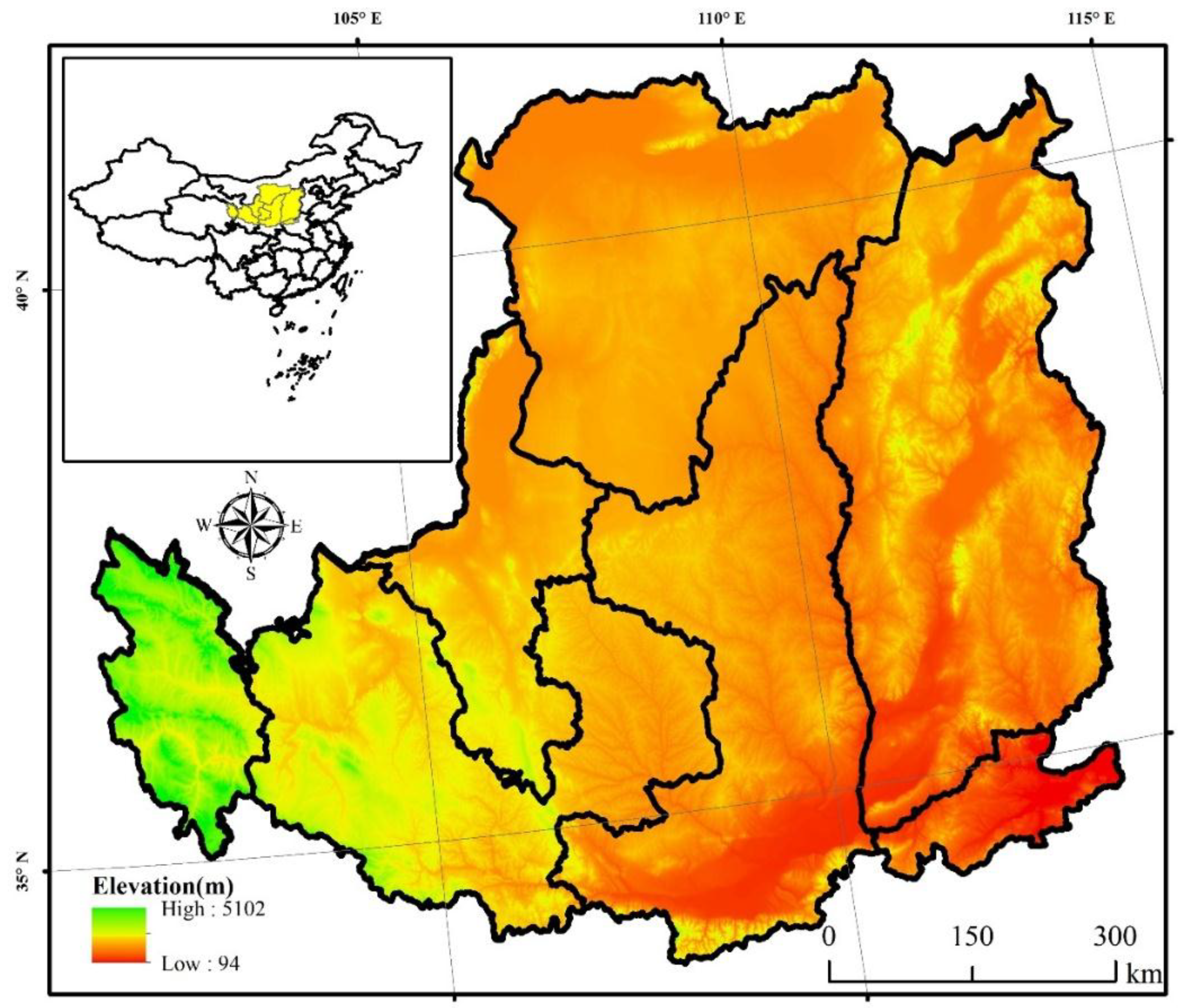
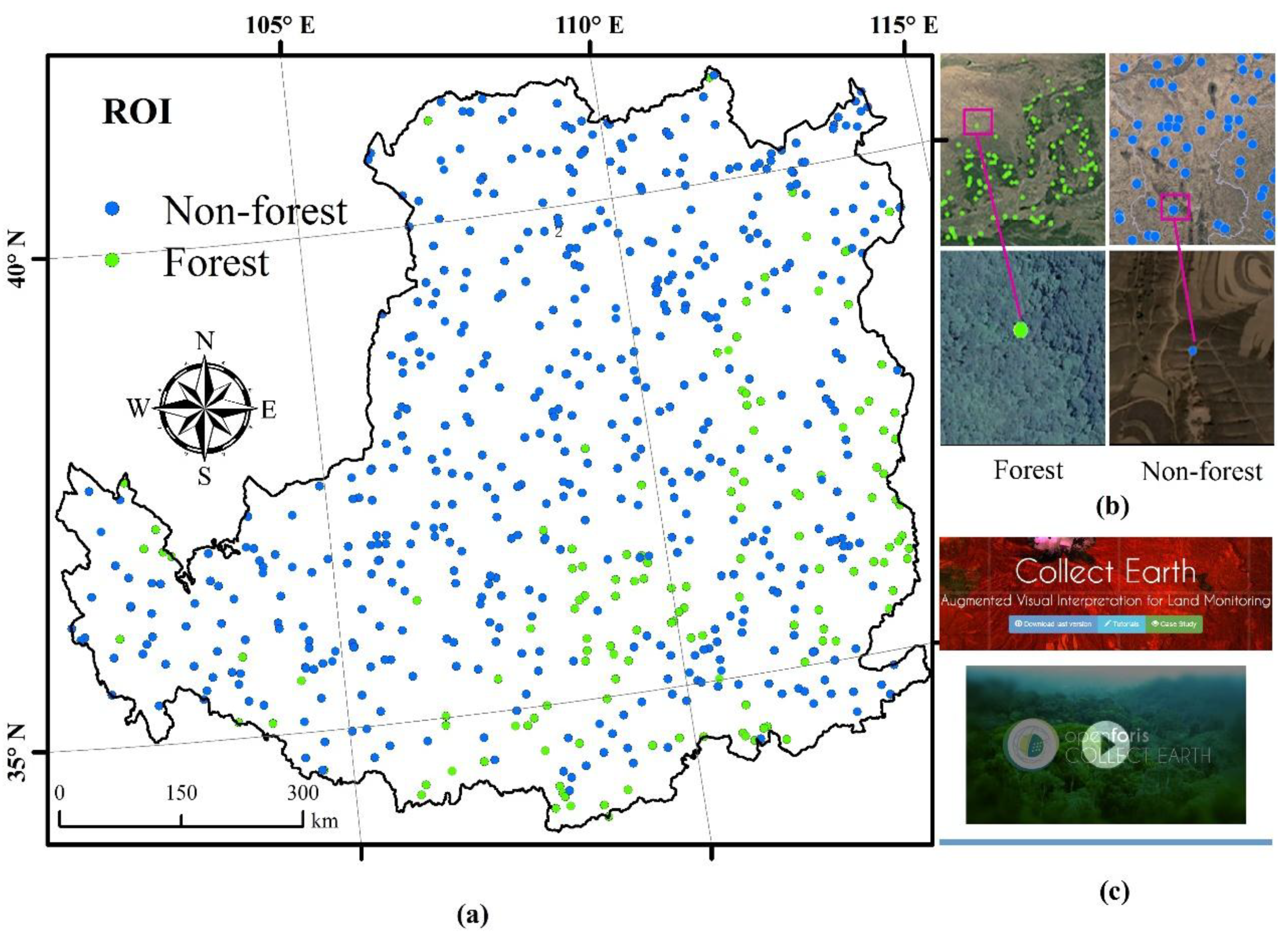
2.1. Study Area
2.2. Data Preprocessing
2.2.1. PALSAR Dataset and Preprocessing
2.2.2. Landsat Images and Preprocessing
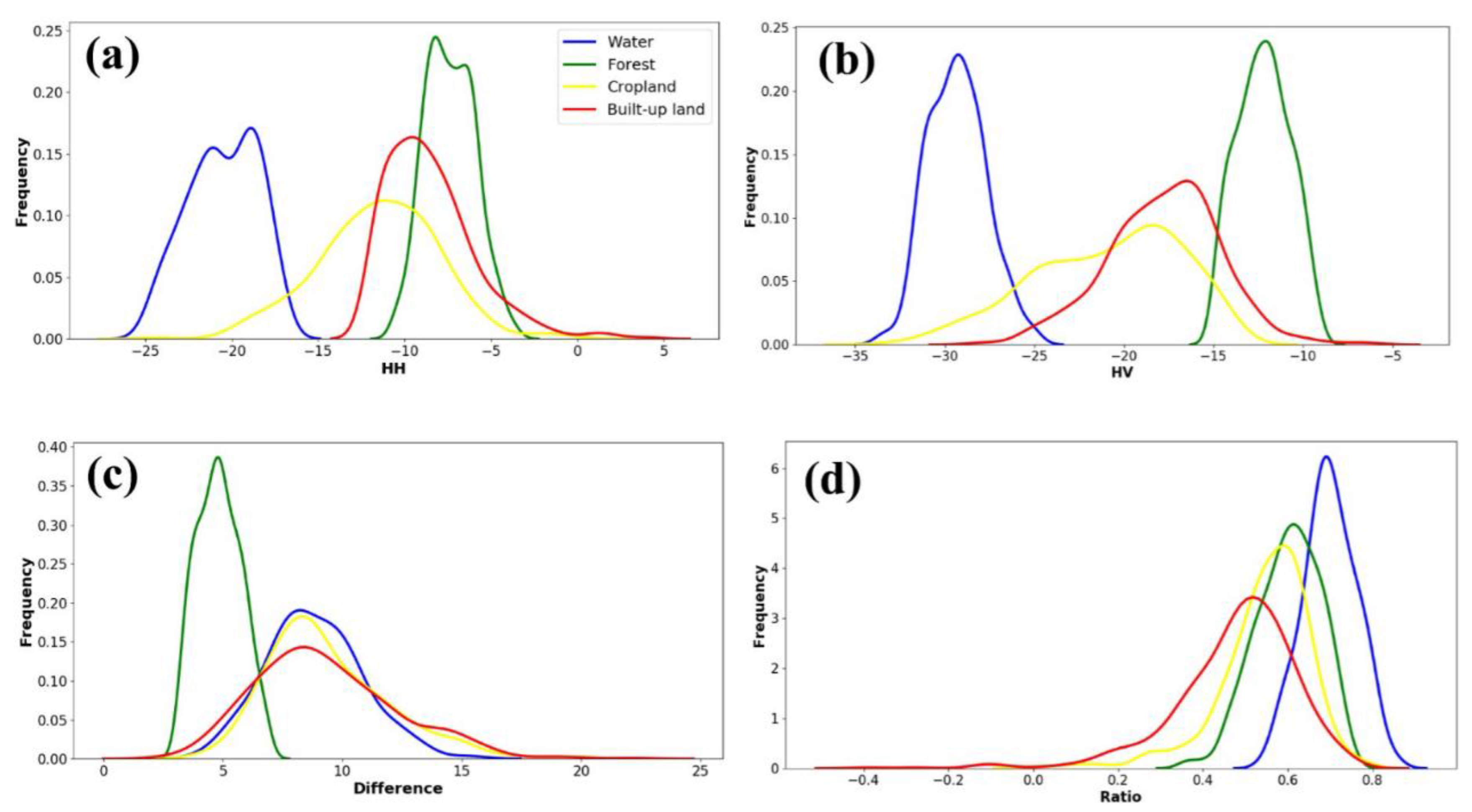
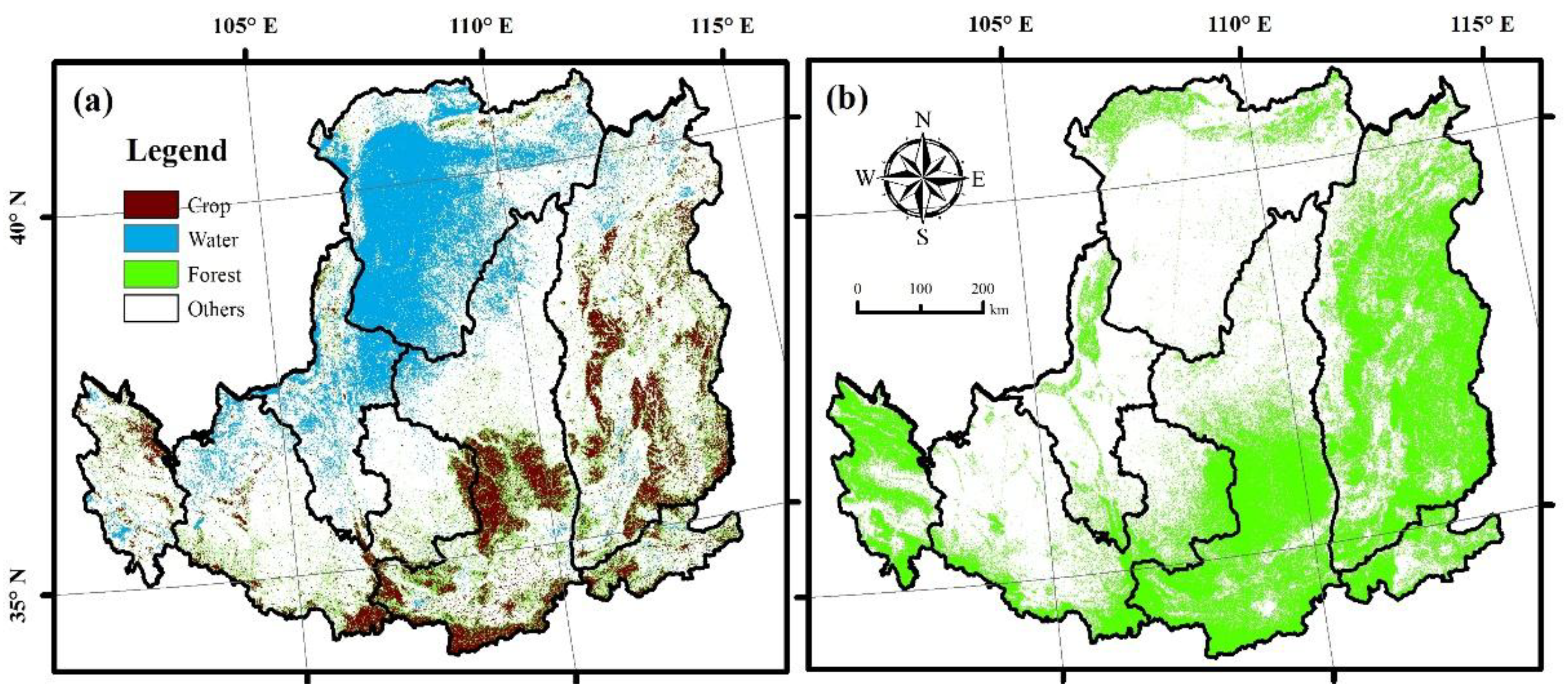
2.3. Mapping Algorithms
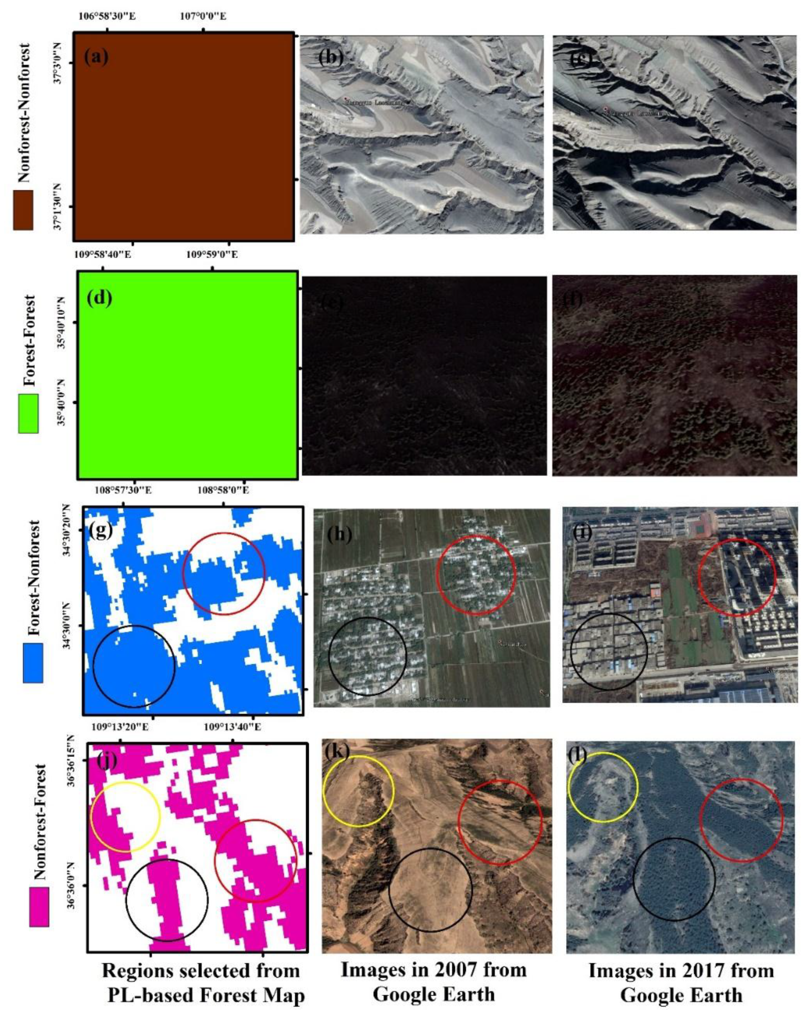
2.4. Validation Samples for Accuracy Assessment of PALSAR/Landsat Forest Maps
2.5. Accuracy Assessment and Comparison with Other Forest Maps
3. Results
3.1. Accuracy of the PL-Based and the Other Five Forest Maps
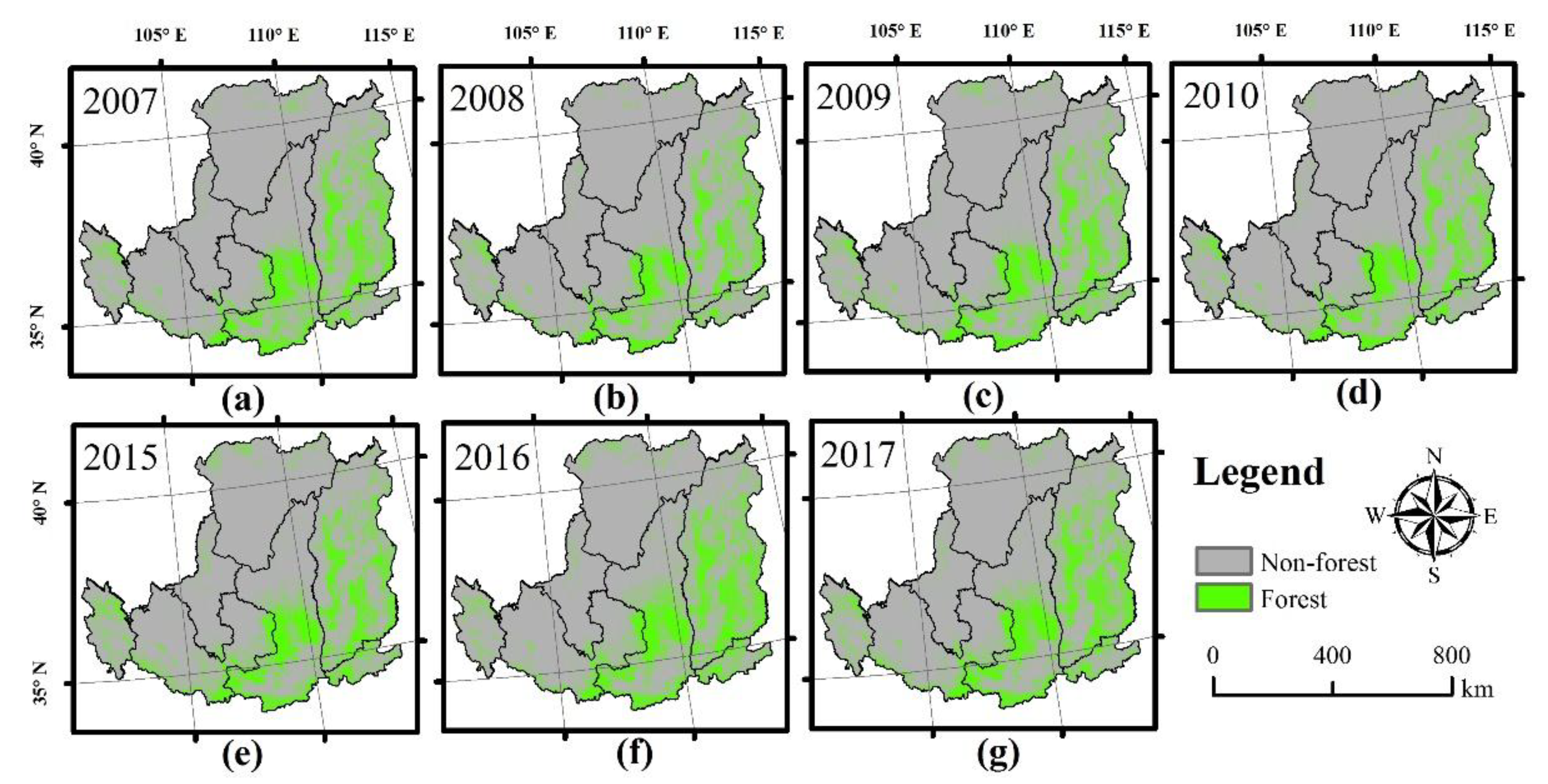
3.2. Changes in Area of Forest Cover in LP from 2007 to 2017
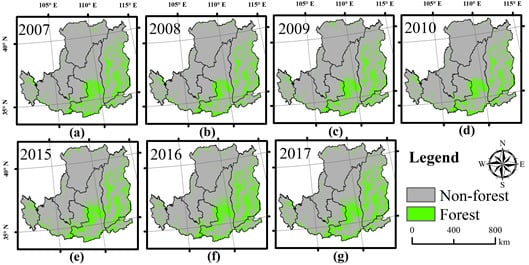
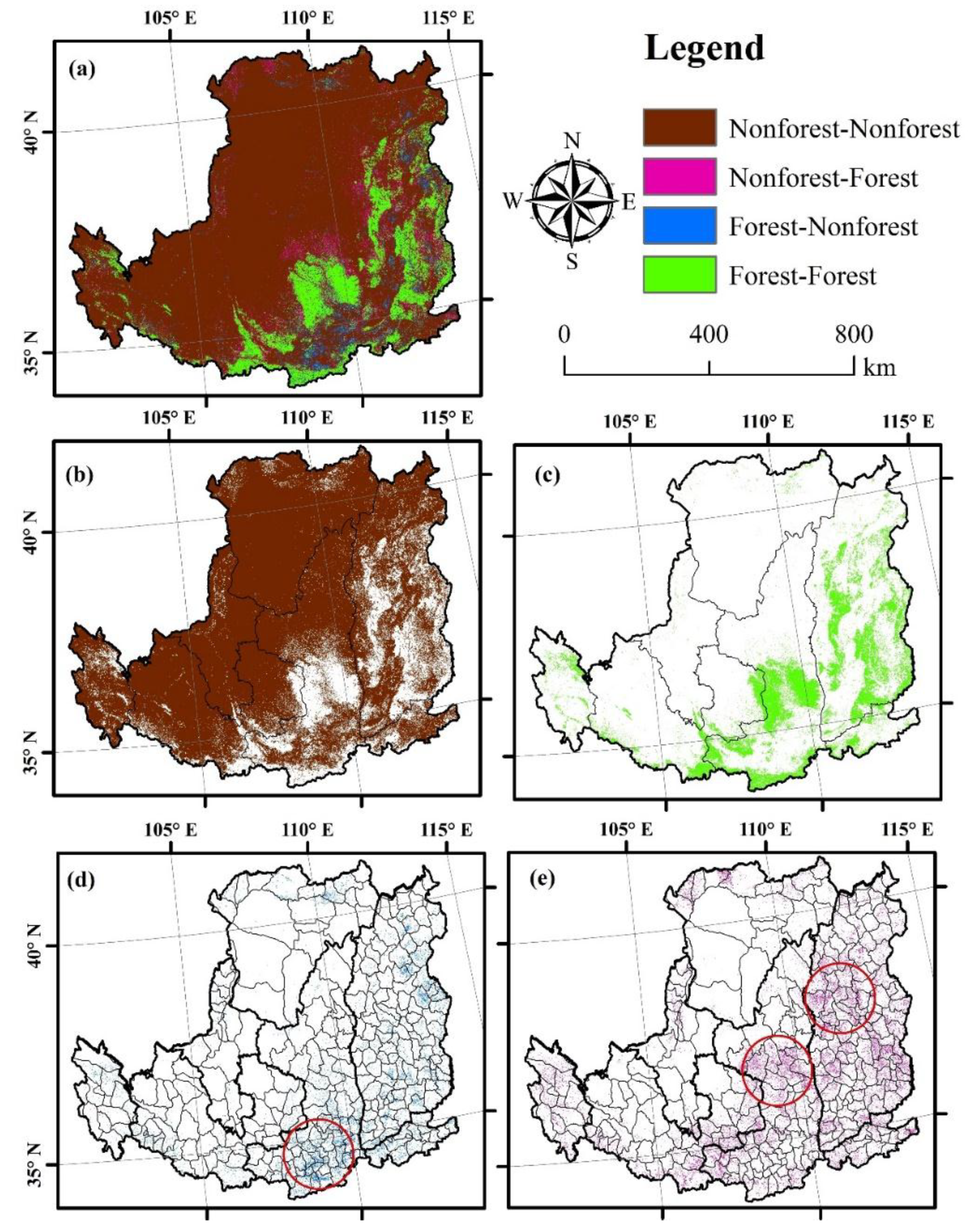
3.3. Changes in Spatial Pattern of the Forest Cover in LP from 2007 to 2017
3.4. Difference among Different Counties in the Loess Plateau
4. Discussion
4.1. Advantage of the PALSAR/Landsat Forest Map Compared to Other Data Forest Maps
4.2. Uncertainty of the Study
5. Conclusions
Author Contributions
Funding
Acknowledgments
Conflicts of Interest
References
- Sexton, J.O.; Noojipady, P.; Song, X.P.; Feng, M.; Song, D.X.; Kim, D.H.; Anand, A.; Huang, C.; Channan, S.; Pimm, S.L. Conservation policy and the measurement of forests. Nat. Clim. Chang. 2015, 6, 192. [Google Scholar] [CrossRef]
- Qin, Y.; Xiao, X.; Dong, J.; Zhang, G.; Roy, P.S.; Joshi, P.K.; Gilani, H.; Murthy, M.S.; Jin, C.; Wang, J. Mapping forests in monsoon Asia with ALOS PALSAR 50-m mosaic images and MODIS imagery in 2010. Sci. Rep. 2016, 6, 20880. [Google Scholar] [CrossRef] [PubMed]
- van der Werf, G.R.; Morton, D.C.; DeFries, R.S.; Olivier, J.G.J.; Kasibhatla, P.S.; Jackson, R.B.; Collatz, G.J.; Randerson, J.T. CO2 emissions from forest loss. Nat. Geosci. 2009, 2, 737–738. [Google Scholar] [CrossRef]
- Houghton, R.A.; Goetz, S.J. New satellites help quantify carbon sources and sinks. Eos Trans. Am. Geophys. Union 2013, 89, 417–418. [Google Scholar] [CrossRef]
- Lu, Y.H.; Fu, B.J.; Feng, X.M.; Zeng, Y.; Liu, Y.; Chang, R.Y.; Sun, G.; Wu, B.F. A policy-driven large scale ecological restoration: Quantifying ecosystem services changes in the Loess Plateau of China. PLos ONE 2012, 7, e31782. [Google Scholar]
- Kim, D.H.; Sexton, J.O.; Noojipady, P.; Huang, C.Q.; Anand, A.; Channan, S.; Feng, M.; Townshend, J.R. Global, Landsat-based forest-cover change from 1990 to 2000. Remote Sens. Environ. 2014, 155, 178–193. [Google Scholar] [CrossRef]
- Hansen, M.C.; Defries, R.S. Detecting long-term global forest change using continuous fields of tree-cover maps from 8-km Advanced Very High Resolution Radiometer (AVHRR) data for the years 1982–99. Ecosystems 2004, 7, 695–716. [Google Scholar] [CrossRef]
- Hansen, M.C.; DeFries, R.S.; Townshend, J.R.G.; Carroll, M.; Dimiceli, C.; Sohlberg, R.A. Global percent tree cover at a spatial resolution of 500 meters: First results of the MODIS vegetation continuous fields algorithm. Earth Interact. 2003, 7, 1–15. [Google Scholar] [CrossRef]
- Hansen, M.C.; Stehman, S.V.; Potapov, P.V.; Loveland, T.R.; Townshend, J.R.G.; DeFries, R.S.; Pittman, K.W.; Arunarwati, B.; Stolle, F.; Steininger, M.K.; et al. Humid tropical forest clearing from 2000 to 2005 quantified by using multitemporal and multiresolution remotely sensed data. Proc. Natl. Acad. Sci. USA 2008, 105, 9439–9444. [Google Scholar] [CrossRef]
- Friedl, M.A.; Sulla-Menashe, D.; Tan, B.; Schneider, A.; Ramankutty, N.; Sibley, A.; Huang, X.M. MODIS collection 5 global land cover: Algorithm refinements and characterization of new datasets. Remote Sens. Environ. 2010, 114, 168–182. [Google Scholar] [CrossRef]
- Yang, Z.Q.; Dong, J.W.; Liu, J.Y.; Zhai, J.; Kuang, W.H.; Zhao, G.S.; Shen, W.; Zhou, Y.; Qin, Y.W.; Xiao, X.M. Accuracy assessment and inter-comparison of eight medium resolution forest products on the Loess Plateau, China. ISPRS Int. J. Geo Inf. 2017, 6, 152. [Google Scholar] [CrossRef]
- Hansen, M.C.; Potapov, P.V.; Moore, R.; Hancher, M.; Turubanova, S.A.; Tyukavina, A.; Thau, D.; Stehman, S.V.; Goetz, S.J.; Loveland, T.R.; et al. High-resolution global maps of 21st-century forest cover change. Science 2013, 342, 850–853. [Google Scholar] [CrossRef] [PubMed]
- Townshend, J.R.; Masek, J.G.; Huang, C.Q.; Vermote, E.F.; Gao, F.; Channan, S.; Sexton, J.O.; Feng, M.; Narasimhan, R.; Kim, D.; et al. Global characterization and monitoring of forest cover using Landsat data: Opportunities and challenges. Int. J. Digit. Earth 2012, 5, 373–397. [Google Scholar] [CrossRef]
- Homer, C.; Dewitz, J.; Yang, L.M.; Jin, S.; Danielson, P.; Xian, G.; Coulston, J.; Herold, N.; Wickham, J.; Megown, K. Completion of the 2011 national land cover database for the conterminous United States—Representing a decade of land cover change information. Photogramm. Eng. Remote Sens. 2015, 81, 345–354. [Google Scholar]
- Jin, S.M.; Yang, L.M.; Danielson, P.; Homer, C.; Fry, J.; Xian, G. A comprehensive change detection method for updating the National Land Cover Database to circa 2011. Remote Sens. Environ. 2013, 132, 159–175. [Google Scholar] [CrossRef]
- Asner, G.P. Cloud cover in Landsat observations of the Brazilian Amazon. Int. J. Remote Sens. 2001, 22, 3855–3862. [Google Scholar] [CrossRef]
- Bastin, J.F.; Berrahmouni, N.; Grainger, A.; Maniatis, D.; Mollicone, D.; Moore, R.; Patriarca, C.; Picard, N.; Sparrow, B.; Abraham, E.M.; et al. The extent of forest in dryland biomes. Science 2017, 356, 635–638. [Google Scholar] [CrossRef]
- Kovacs, J.M.; Lu, X.X.; Flores-Verdugo, F.; Zhang, C.; de Santiago, F.F.; Jiao, X. Applications of ALOS PALSAR for monitoring biophysical parameters of a degraded black mangrove (Avicennia germinans) forest. ISPRS J. Photogramm. 2013, 82, 102–111. [Google Scholar] [CrossRef]
- Ni, W.J.; Sun, G.Q.; Guo, Z.F.; Zhang, Z.Y.; He, Y.T.; Huang, W.L. Retrieval of forest biomass from ALOS PALSAR data using a lookup table method. IEEE J. Stars 2013, 6, 875–886. [Google Scholar] [CrossRef]
- Lucas, R.M.; Cronin, N.; Lee, A.; Moghaddam, M.; Witte, C.; Tickle, P. Empirical relationships between AIRSAR backscatter and LiDAR-derived forest biomass, queensland, Australia. Remote Sens. Environ. 2006, 100, 407–425. [Google Scholar] [CrossRef]
- Baghdadi, N.; Boyer, N.; Todoroff, P.; El Hajj, M.; Begue, A. Potential of SAR sensors TerraSAR-X, ASAR/ENVISAT and PALSAR/ALOS for monitoring sugarcane crops on Reunion Island. Remote Sens. Environ. 2009, 113, 1724–1738. [Google Scholar] [CrossRef]
- Shimada, M.; Itoh, T.; Motooka, T.; Watanabe, M.; Shiraishi, T.; Thapa, R.; Lucas, R. New global forest/non-forest maps from ALOS PALSAR data (2007–2010). Remote Sens. Environ. 2014, 155, 13–31. [Google Scholar] [CrossRef]
- Ju, J.C.; Roy, D.P. The availability of cloud-free Landsat ETM plus data over the conterminous United States and globally. Remote Sens. Environ. 2008, 112, 1196–1211. [Google Scholar] [CrossRef]
- Chen, B.Q.; Li, X.P.; Xiao, X.M.; Zhao, B.; Dong, J.W.; Kou, W.L.; Qin, Y.W.; Yang, C.; Wu, Z.X.; Sun, R.; et al. Mapping tropical forests and deciduous rubber plantations in Hainan Island, China by integrating PALSAR 25-m and multi-temporal Landsat images. Int. J. Appl. Earth Obs. 2016, 50, 117–130. [Google Scholar] [CrossRef]
- Dong, J.W.; Xiao, X.M.; Sheldon, S.; Biradar, C.; Duong, N.D.; Hazarika, M. A comparison of forest cover maps in Mainland Southeast Asia from multiple sources: PALSAR, MERIS, MODIS and FRA. Remote Sens. Environ. 2012, 127, 60–73. [Google Scholar] [CrossRef]
- Qin, Y.W.; Xiao, X.M.; Dong, J.W.; Zhang, G.L.; Shimada, M.; Liu, J.Y.; Li, C.G.; Kou, W.L.; Moore, B. Forest cover maps of China in 2010 from multiple approaches and data sources: PALSAR, Landsat, MODIS, FRA, and NFI. ISPRS J. Photogramm. 2015, 109, 1–16. [Google Scholar] [CrossRef]
- Qin, Y.; Xiao, X.; Dong, J.; Zhou, Y.; Wang, J.; Doughty, R.B.; Chen, Y.; Zou, Z.; Moore, B. Annual dynamics of forest areas in South America during 2007–2010 at 50-m spatial resolution. Remote Sens. Environ. 2017, 201, 73–87. [Google Scholar] [CrossRef]
- Qin, Y.W.; Xiao, X.M.; Wang, J.; Dong, J.W.; Ewing, K.T.; Hoagland, B.; Hough, D.J.; Fagin, T.D.; Zou, Z.H.; Geissler, G.L.; et al. Mapping annual forest cover in sub-humid and semi-arid regions through analysis of landsat and PALSAR imagery. Remote Sens. 2016, 8, 933. [Google Scholar] [CrossRef]
- Yang, Z.; Dong, J.; Qin, Y.; Ni, W.; Zhao, G.; Chen, W.; Chen, B.; Kou, W.; Wang, J.; Xiao, X. Integrated analyses of PALSAR and landsat imagery reveal more agroforests in a typical agricultural production region, North China Plain. Remote Sens. 2018, 10, 1323. [Google Scholar] [CrossRef]
- Reiche, J.; Lucas, R.; Mitchell, A.L.; Verbesselt, J.; Hoekman, D.H.; Haarpaintner, J.; Kellndorfer, J.M.; Rosenqvist, A.; Lehmann, E.A.; Woodcock, C.E.; et al. Combining satellite data for better tropical forest monitoring. Nat. Clim. Chang. 2016, 6, 120–122. [Google Scholar] [CrossRef]
- Cai, Q.G. Soil erosion and management on the Loess Plateau. J. Geogr. Sci. 2001, 11, 53–70. [Google Scholar]
- Zhang, X.C.; Liu, W.Z. Simulating potential response of hydrology, soil erosion, and crop productivity to climate change in Changwu tableland region on the Loess Plateau of China. Agric. For. Meteorol. 2005, 131, 127–142. [Google Scholar] [CrossRef]
- Wang, Y.Q.; Shao, M.A.; Liu, Z.P. Large-scale spatial variability of dried soil layers and related factors across the entire Loess Plateau of China. Geoderma 2010, 159, 99–108. [Google Scholar] [CrossRef]
- Shimada, M.; Ohtaki, T. Generating large-scale high-quality SAR mosaic datasets: Application to PALSAR data for global monitoring. IEEE J. Stars 2010, 3, 637–656. [Google Scholar] [CrossRef]
- Rosenqvist, A.; Shimada, M.; Ito, N.; Watanabe, M. ALOS PALSAR: A pathfinder mission for global-scale monitoring of the environment. IEEE Trans. Geosci. Remote Sens. 2007, 45, 3307–3316. [Google Scholar] [CrossRef]
- Shimada, M.; Isoguchi, O.; Tadono, T.; Isono, K. PALSAR Radiometric and geometric calibration. IEEE Trans. Geosci. Remote Sens. 2009, 47, 3915–3932. [Google Scholar] [CrossRef]
- Walker, W.S.; Stickler, C.M.; Kellndorfer, J.M.; Kirsch, K.M.; Nepstad, D.C. Large-area classification and mapping of forest and land cover in the Brazilian Amazon: A comparative analysis of ALOS/PALSAR and landsat data sources. IEEE J. Stars 2010, 3, 594–604. [Google Scholar] [CrossRef]
- Miettinen, J.; Liew, S.C. Separability of insular Southeast Asian woody plantation species in the 50 m resolution ALOS PALSAR mosaic product. Remote Sens. Lett. 2011, 2, 299–307. [Google Scholar] [CrossRef]
- Gamon, J.A.; Field, C.B.; Goulden, M.L.; Griffin, K.L.; Hartley, A.E.; Joel, G.; Peñuelas, J.; Valentini, R. Relationships between NDVI, canopy structure, and photosynthesis in three Californian vegetation types. Ecol. Appl. 1995, 5, 28–41. [Google Scholar] [CrossRef] [Green Version]
- Zhu, Z.; Woodcock, C.E. Automated cloud, cloud shadow, and snow detection in multitemporal Landsat data: An algorithm designed specifically for monitoring land cover change. Remote Sens. Environ. 2014, 152, 217–234. [Google Scholar] [CrossRef]
- Zhe, Z.; Wang, S.; Woodcock, C.E. Improvement and expansion of the Fmask algorithm: Cloud, cloud shadow, and snow detection for Landsats 4–7, 8, and Sentinel 2 images. Remote Sens. Environ. 2015, 159, 269–277. [Google Scholar] [CrossRef]
- Potere, D. Horizontal positional accuracy of Google Earth’s high-resolution imagery archive. Sensors 2008, 8, 7973–7981. [Google Scholar] [CrossRef] [PubMed]
- Viña, A.; Mcconnell, W.J.; Yang, H.; Xu, Z.; Liu, J. Effects of conservation policy on China’s forest recovery. Sci. Adv. 2016, 2, e1500965. [Google Scholar] [CrossRef] [PubMed] [Green Version]
- Wennberg, A. Food and Agriculture Organization of the United Nations 2014; FAO of the UN: Rome, Italy, 2014. [Google Scholar]
- Liu, J.Y.; Kuang, W.H.; Zhang, Z.X.; Xu, X.L.; Qin, Y.W.; Ning, J.; Zhou, W.C.; Zhang, S.W.; Li, R.D.; Yan, C.Z.; et al. Spatiotemporal characteristics, patterns, and causes of land-use changes in China since the late 1980s. J. Geogr. Sci. 2014, 24, 195–210. [Google Scholar] [CrossRef]
- Yang, Y.K.; Xiao, P.F.; Feng, X.Z.; Li, H.X. Accuracy assessment of seven global land cover datasets over China. ISPRS J. Photogramm. 2017, 125, 156–173. [Google Scholar] [CrossRef]
- Mayaux, P.; Eva, H.; Gallego, J.; Strahler, A.H.; Herold, M.; Agrawal, S.; Naumov, S.; De Miranda, E.E.; Di Bella, C.M.; Ordoyne, C.; et al. Validation of the global land cover 2000 map. IEEE Trans. Geosci. Remote Sens. 2006, 44, 1728–1739. [Google Scholar] [CrossRef] [Green Version]
- Gong, P.; Wang, J.; Yu, L.; Zhao, Y.C.; Zhao, Y.Y.; Liang, L.; Niu, Z.G.; Huang, X.M.; Fu, H.H.; Liu, S.; et al. Finer resolution observation and monitoring of global land cover: First mapping results with Landsat TM and ETM+ data. Int. J. Remote Sens. 2013, 34, 2607–2654. [Google Scholar] [CrossRef] [Green Version]
- Chen, J.; Chen, J.; Liao, A.P.; Cao, X.; Chen, L.J.; Chen, X.H.; He, C.Y.; Han, G.; Peng, S.; Lu, M.; et al. Global land cover mapping at 30 m resolution: A POK-based operational approach. ISPRS J. Photogramm. 2015, 103, 7–27. [Google Scholar] [CrossRef] [Green Version]
- Sexton, J.O.; Song, X.P.; Feng, M.; Noojipady, P.; Anand, A.; Huang, C.Q.; Kim, D.H.; Collins, K.M.; Channan, S.; DiMiceli, C.; et al. Global, 30-m resolution continuous fields of tree cover: Landsat-based rescaling of MODIS vegetation continuous fields with lidar-based estimates of error. Int. J. Digit. Earth 2013, 6, 427–448. [Google Scholar] [CrossRef] [Green Version]
- Olofsson, P.; Foody, G.M.; Herold, M.; Stehman, S.V.; Woodcock, C.E.; Wulder, M.A. Good practices for estimating area and assessing accuracy of land change. Remote Sens. Environ. 2014, 148, 42–57. [Google Scholar] [CrossRef]
- Xiao, J. Satellite evidence for significant biophysical consequences of the “Grain for Green” Program on the Loess Plateau in China. J. Geophys. Res. Biogeosci. 2015, 119, 2261–2275. [Google Scholar] [CrossRef] [Green Version]
- Asner, G.P.; Knapp, D.E.; Broadbent, E.N.; Oliveira, P.J.C.; Keller, M.; Silva, J.N. Selective logging in the Brazilian Amazon. Science 2005, 310, 480–482. [Google Scholar] [CrossRef] [PubMed]
- Cao, S.; Chen, L.I.; Chenguang, X.U.; Liu, Z. Impact of three soil types on afforestation in China’s Loess Plateau: Growth and survival of six tree species and their effects on soil properties. Landsc. Urban Plan. 2007, 83, 208–217. [Google Scholar] [CrossRef]
- Cao, S.; Li, C.; Shankman, D.; Wang, C.; Wang, X.; Hong, Z. Excessive reliance on afforestation in China’s arid and semi-arid regions: Lessons in ecological restoration. Earth Sci. Rev. 2011, 104, 240–245. [Google Scholar] [CrossRef]
- Peng, S.S.; Piao, S.L.; Zeng, Z.Z.; Ciais, P.; Zhou, L.M.; Li, L.Z.X.; Myneni, R.B.; Yin, Y.; Zeng, H. Afforestation in China cools local land surface temperature. Proc. Natl. Acad. Sci. USA 2014, 111, 2915–2919. [Google Scholar] [CrossRef] [Green Version]


| Main Scale of the PALSAR | ||||
|---|---|---|---|---|
| Mode | High Resolution | Scanning Synthetic Aperture | Polarization | |
| Center frequency | 1270 MHz (L-band) | |||
| Linear frequency modulation width | 28 MHz | 14 MHz | 14 MHz, 28 MHz | 14 MHz |
| Polarization mode | HH or VV | HH + HV or VV + VH | HH or VV | HH + HV + VH + VV |
| Incident angle | 8°–60° | 8°–60° | 18°–43° | 8°–30° |
| Spatial resolution | 7–44 m | 14–88 m | 100 m | 24–89 m |
| Width | 40–70 km | 40–70 km | 250–350 km | 20–65 km |
| Satellite parameters of the Landsat | ||||
| Satellite parameters | TM sensor | |||
| Country | United States | Band | Wavelength range (μm) | Resolution (m) |
| Design life | 5 | 1 | 0.45~0.53 | 30 |
| Launch time | 1994-04-15 | 2 | 0.52~0.60 | 30 |
| Estimated time to failure | 3 | 0.63~0.69 | 30 | |
| Track type | Near-polar sun synchronization orbit | 4 | 0.76~0.90 | 30 |
| Track height | 705 km | 5 | 1.55~1.75 | 30 |
| Orbital inclination | 98.2° | 6 | 10.40~12.50 | 60 |
| Operation cycle | 98.9 min | 7 | 2.09~2.35 | 30 |
| Around the earth every day | 15 | 8 | 0.52~0.90 | 15 |
| Forest Maps | Forest Cover Types | Resolution | Algorithms | Data Sources | Major References |
|---|---|---|---|---|---|
| FROM-GLC | Tree cover ≥ 15%, Tree height ≥ 3 m | 30 m | Automatic classification algorithms | Landsat | [48] |
| GlobeLand30 | Tree cover ≥ 10% | 30 m | POK(pixel-object-konwledge)-based method | Landsat, HJ-1 | [49] |
| GLCF-VCF | Tree cover ≥ 10%, Tree height ≥ 5 m | 30 m | Supervised classification | Landsat | [50] |
| JAXA | Tree cover ≥ 10%, Tree height ≥ 5 m | 25 m | Rule-based | PALSAR | [22] |
| OU-FDL | Tree cover ≥ 10%, Tree height ≥ 5 m | 30 m | Decision Tree | PALSAR, MODIS | [26] |
| PALSAR/Landsat | Tree cover ≥ 10%, Tree height ≥ 5 m | 30 m | Rule-based | PALSAR, Landsat | This study |
| Forest Maps | Type | UA (%) | PA (%) | OA (%) | Kappa |
|---|---|---|---|---|---|
| FROM-GLC | Forest | 81.26 | 71.52 | 87.96 | 0.68 |
| Non-Forest | 90.02 | 93.40 | |||
| GlobeLand30 | Forest | 78.62 | 71.22 | 87.47 | 0.66 |
| Non-Forest | 90.20 | 93.19 | |||
| GLCF-VCF | Forest | 72.33 | 67.30 | 85.20 | 0.60 |
| Non-Forest | 89.16 | 91.27 | |||
| JAXA | Forest | 59.01 | 67.28 | 83.57 | 0.52 |
| Non-Forest | 91.15 | 87.82 | |||
| OU-FDL | Forest | 65.30 | 67.47 | 84.40 | 0.56 |
| Non-Forest | 90.29 | 89.41 | |||
| PALSAR/Landsat | Forest | 91.07 | 76.41 | 91.27 | 0.77 |
| Non-Forest | 91.33 | 97.07 |
© 2019 by the authors. Licensee MDPI, Basel, Switzerland. This article is an open access article distributed under the terms and conditions of the Creative Commons Attribution (CC BY) license (http://creativecommons.org/licenses/by/4.0/).
Share and Cite
Zhou, H.; Xu, F.; Dong, J.; Yang, Z.; Zhao, G.; Zhai, J.; Qin, Y.; Xiao, X. Tracking Reforestation in the Loess Plateau, China after the “Grain for Green” Project through Integrating PALSAR and Landsat Imagery. Remote Sens. 2019, 11, 2685. https://doi.org/10.3390/rs11222685
Zhou H, Xu F, Dong J, Yang Z, Zhao G, Zhai J, Qin Y, Xiao X. Tracking Reforestation in the Loess Plateau, China after the “Grain for Green” Project through Integrating PALSAR and Landsat Imagery. Remote Sensing. 2019; 11(22):2685. https://doi.org/10.3390/rs11222685
Chicago/Turabian StyleZhou, Hui, Fu Xu, Jinwei Dong, Zhiqi Yang, Guosong Zhao, Jun Zhai, Yuanwei Qin, and Xiangming Xiao. 2019. "Tracking Reforestation in the Loess Plateau, China after the “Grain for Green” Project through Integrating PALSAR and Landsat Imagery" Remote Sensing 11, no. 22: 2685. https://doi.org/10.3390/rs11222685