Author Contributions
The first two authors have equally contributed to the work. Conceptualization, G.S. and D.C.; methodology, G.S., D.C., and P.L.; software, G.S.; validation, G.S., D.C., and P.L.; formal analysis, G.S., D.C., P.L., A.O., and F.R.; investigation, G.S., D.C., P.L., A.O., and F.R.; resources, G.S., D.C., and P.L.; writing—original draft preparation, G.S. and D.C.; writing—review and editing, G.S., D.C., A.O., and F.R.; visualization, G.S., D.C., and P.L.; supervision, G.S. and D.C.; project administration, G.S. and D.C.; funding acquisition, G.S., D.C., A.O., and F.R.
Figure 1.
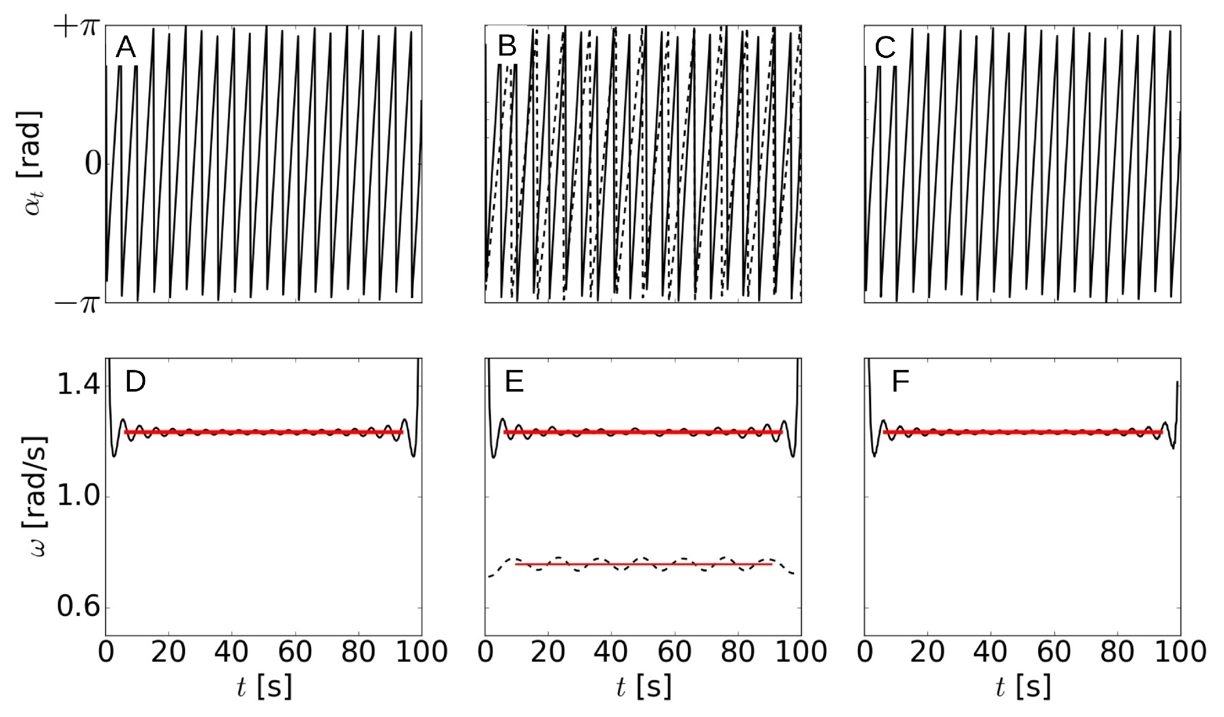
Angle of the Pricipal Component (PC) (A–C) and frequency (D–F) for the monochromatic (A,D), bichromatic (B,E), and reflective (C,F) 1D cases versus time: First (second) mode is in solid (dashed) lines. Red lines are for the mean angular frequencies.
Figure 1.
Angle of the Pricipal Component (PC) (A–C) and frequency (D–F) for the monochromatic (A,D), bichromatic (B,E), and reflective (C,F) 1D cases versus time: First (second) mode is in solid (dashed) lines. Red lines are for the mean angular frequencies.
Figure 2.
Angle of the Empirical Orthogonal Function ((A–C), wavenumber from phase fitting D–F), depth from phase fitting (G–I), function fitting (J–L), and windowing (M–O, with ) for each of the monochromatic, bichromatic, and reflective 1D cases: First (second) mode is in solid (dashed) lines. Blue lines are for the exact depth.
Figure 3.
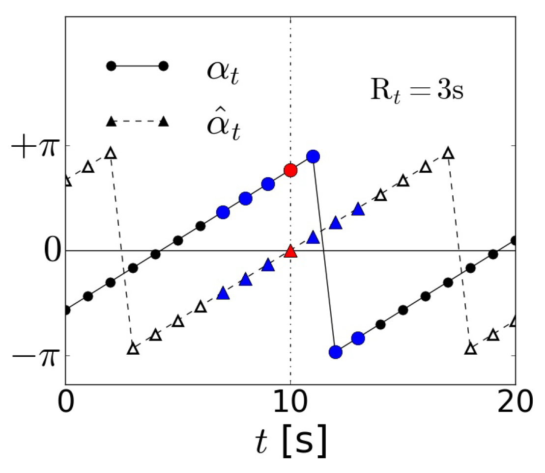
Angle of the PC before centering (circles) and after centering around (triangles) for and : Red denotes the point of interest, and blue indicates the neighbour points used.
Figure 3.
Angle of the PC before centering (circles) and after centering around (triangles) for and : Red denotes the point of interest, and blue indicates the neighbour points used.
Figure 4.
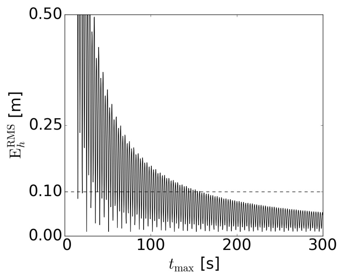
Evolution of the Root Mean Square (RMS) error in h, , as a function of for the monochromatic case using phase fitting (without windowing).
Figure 4.
Evolution of the Root Mean Square (RMS) error in h, , as a function of for the monochromatic case using phase fitting (without windowing).
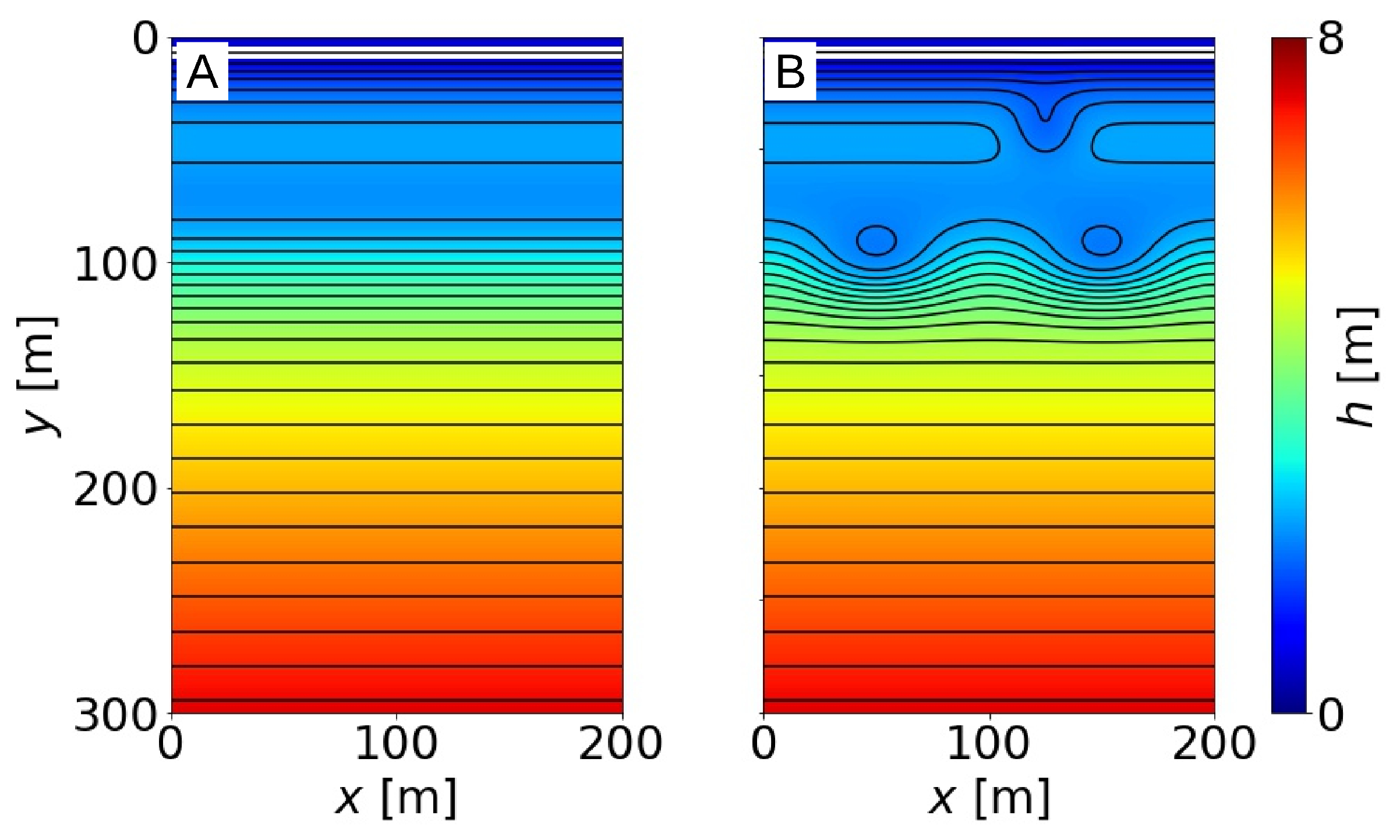
Figure 5.
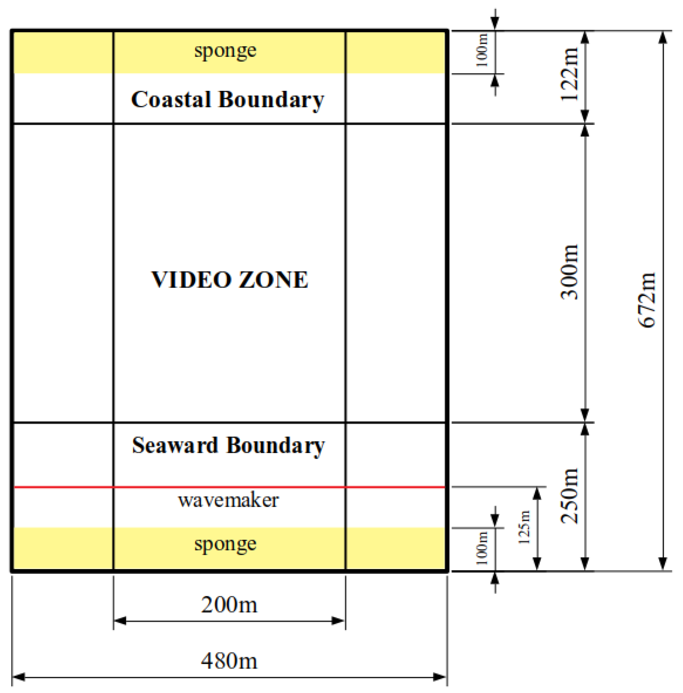
Bathymetries (in meters) for the analysis of linear waves (A) and nonlinear waves (B): The white strip next to the shore highlights .
Figure 5.
Bathymetries (in meters) for the analysis of linear waves (A) and nonlinear waves (B): The white strip next to the shore highlights .
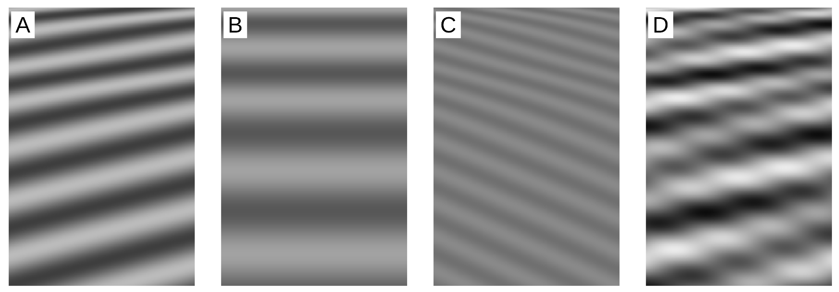
Figure 6.
Initial snapshots for linear synthetic wave trains W1 (A), W2 (B), and W3 (C) and their superposition WS (D): Spatial domain is (in the alongshore and cross-shore directions), and pixel intensity is a linear function of the modelled free surface elevation.
Figure 6.
Initial snapshots for linear synthetic wave trains W1 (A), W2 (B), and W3 (C) and their superposition WS (D): Spatial domain is (in the alongshore and cross-shore directions), and pixel intensity is a linear function of the modelled free surface elevation.
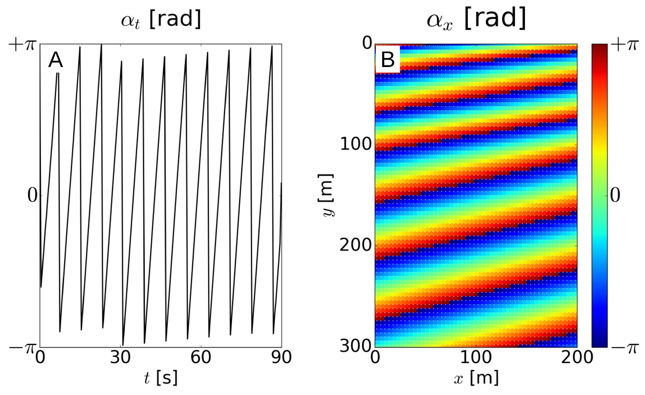
Figure 7.
Angles (A) and (B) of the first PC and EOF corresponding to linear propagation of W1 for and : The explained variance is above .
Figure 7.
Angles (A) and (B) of the first PC and EOF corresponding to linear propagation of W1 for and : The explained variance is above .
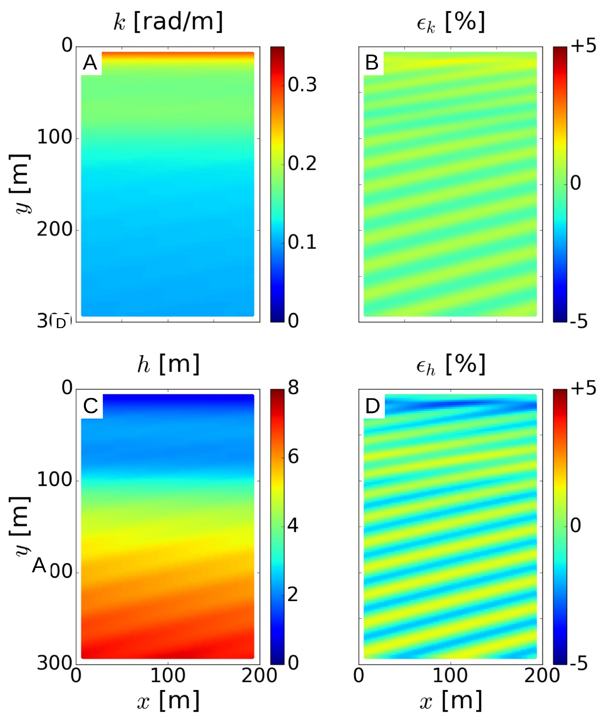
Figure 8.
Recovered k (A) and h (C) and the corresponding local relative errors, and (B,D, in %), obtained using the phase fitting method for the first EOF corresponding to linear propagation of W1 and for , , , and .
Figure 8.
Recovered k (A) and h (C) and the corresponding local relative errors, and (B,D, in %), obtained using the phase fitting method for the first EOF corresponding to linear propagation of W1 and for , , , and .
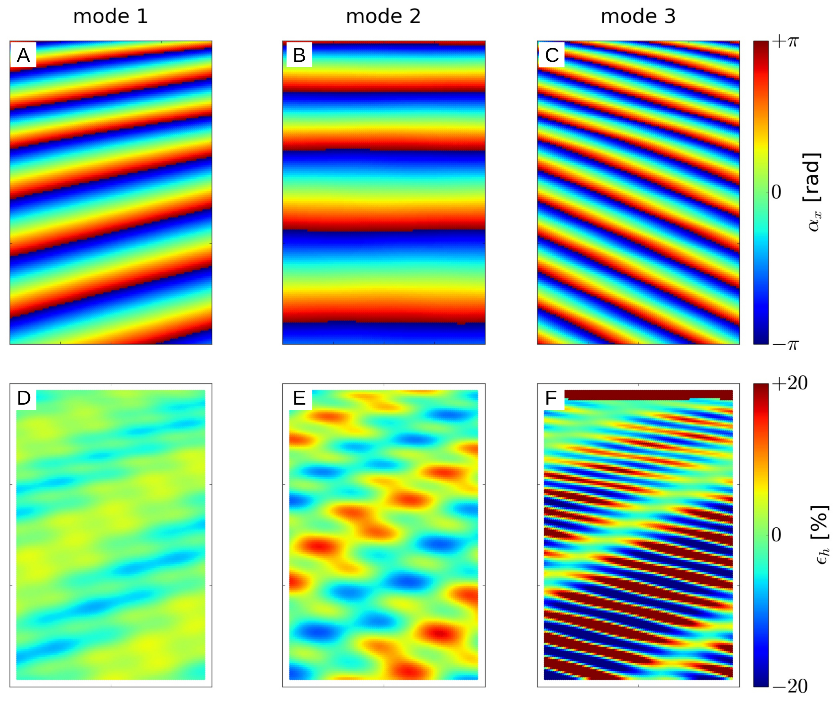
Figure 9.
Phase fitting without windowing of the three modes of the linear polychromatic wave field WS for , , , and : (A–C) and (D–F).
Figure 9.
Phase fitting without windowing of the three modes of the linear polychromatic wave field WS for , , , and : (A–C) and (D–F).
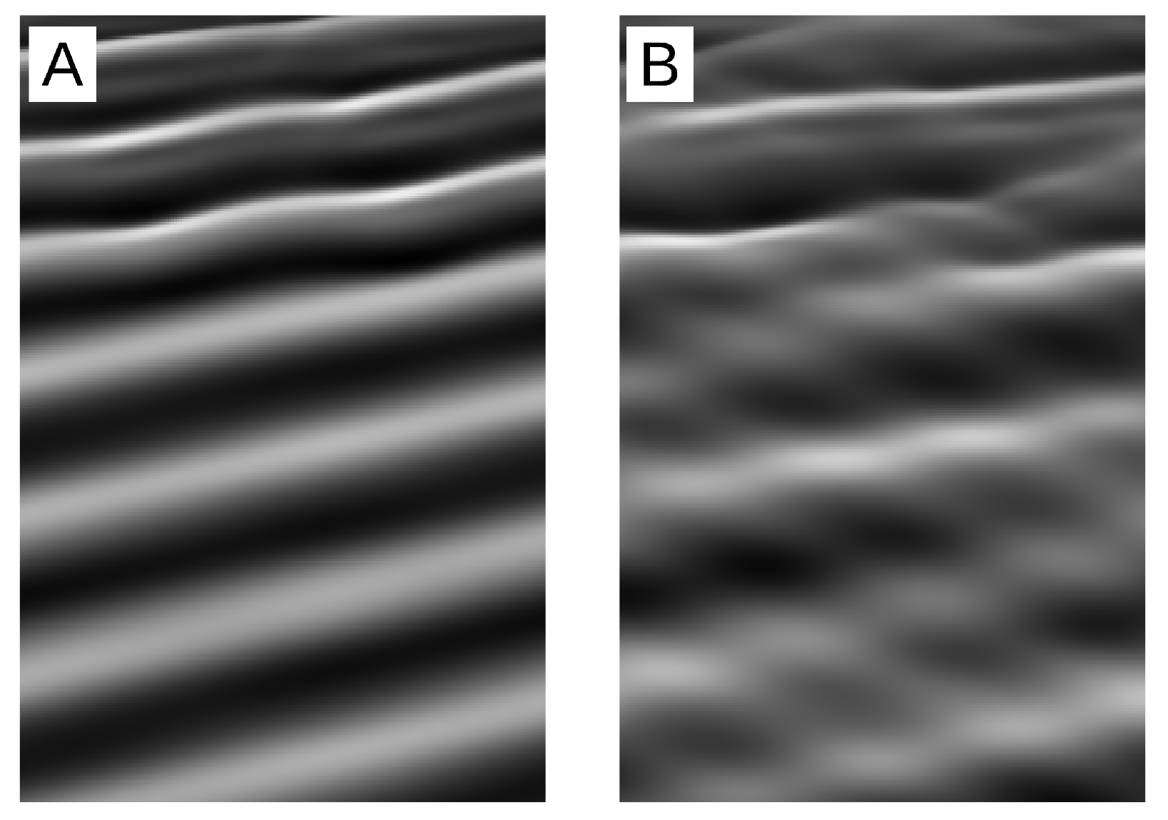
Figure 10.
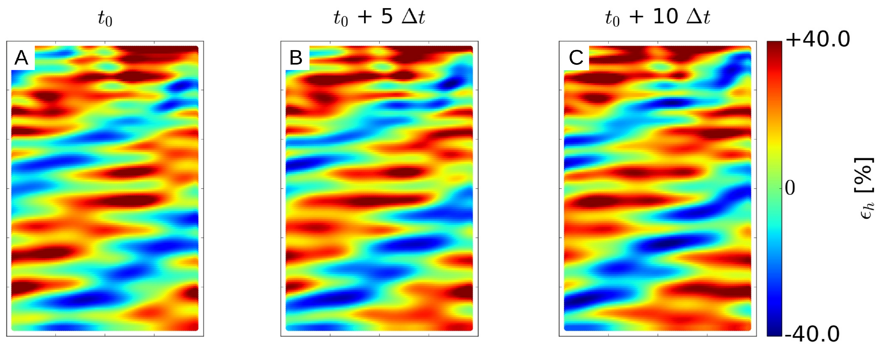
Initial snapshots for synthetic nonlinear wave trains W1 (A) and WS (B) for : Spatial domain is (in the alongshore and cross-shore directions), and pixel intensity is a linear function of the modelled free surface elevation.
Figure 10.
Initial snapshots for synthetic nonlinear wave trains W1 (A) and WS (B) for : Spatial domain is (in the alongshore and cross-shore directions), and pixel intensity is a linear function of the modelled free surface elevation.
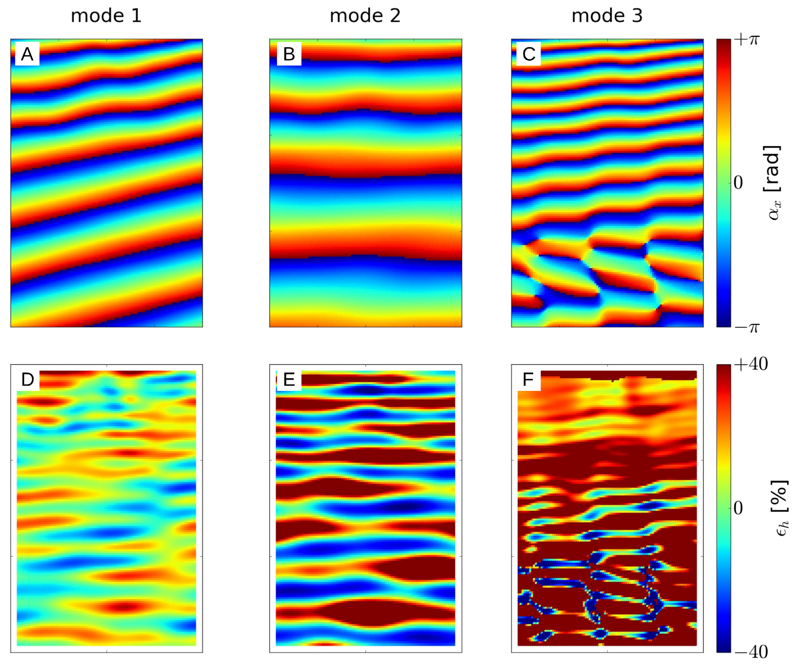
Figure 11.
Results for (A–C) and (D–F) obtained with the phase fitting method without windowing from the nonlinear polychromatic wave field WS with for , , , , and .
Figure 11.
Results for (A–C) and (D–F) obtained with the phase fitting method without windowing from the nonlinear polychromatic wave field WS with for , , , , and .
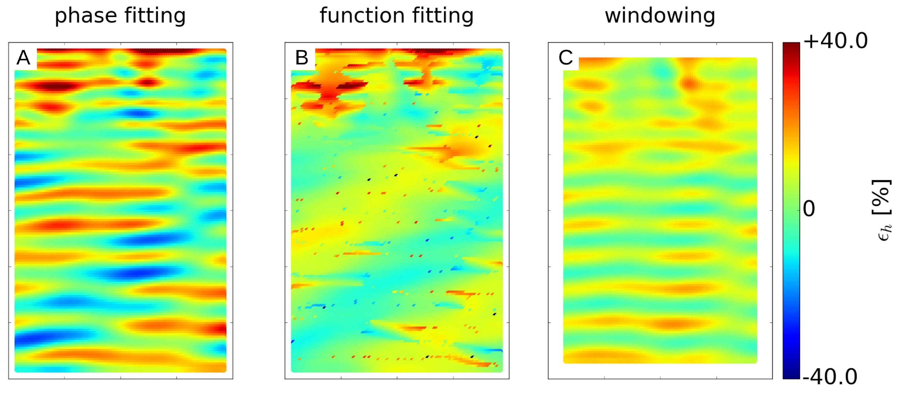
Figure 12.
Results for obtained with phase fitting (A), function fitting (B), and windowing (C, with ) from the first mode for the nonlinear polychromatic wave field WS with , , , , , and .
Figure 12.
Results for obtained with phase fitting (A), function fitting (B), and windowing (C, with ) from the first mode for the nonlinear polychromatic wave field WS with , , , , , and .
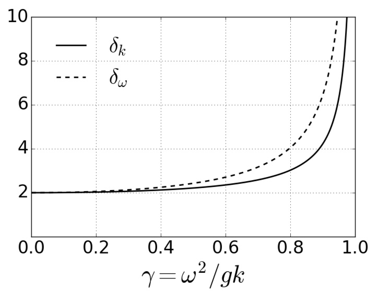
Figure 13.
Propagation of the errors in k and to water depth h when using the dispersion relation.
Figure 13.
Propagation of the errors in k and to water depth h when using the dispersion relation.
Figure 14.
Propagation of the errors in the bathymetry inversion for three time windows.
Figure 14.
Propagation of the errors in the bathymetry inversion for three time windows.
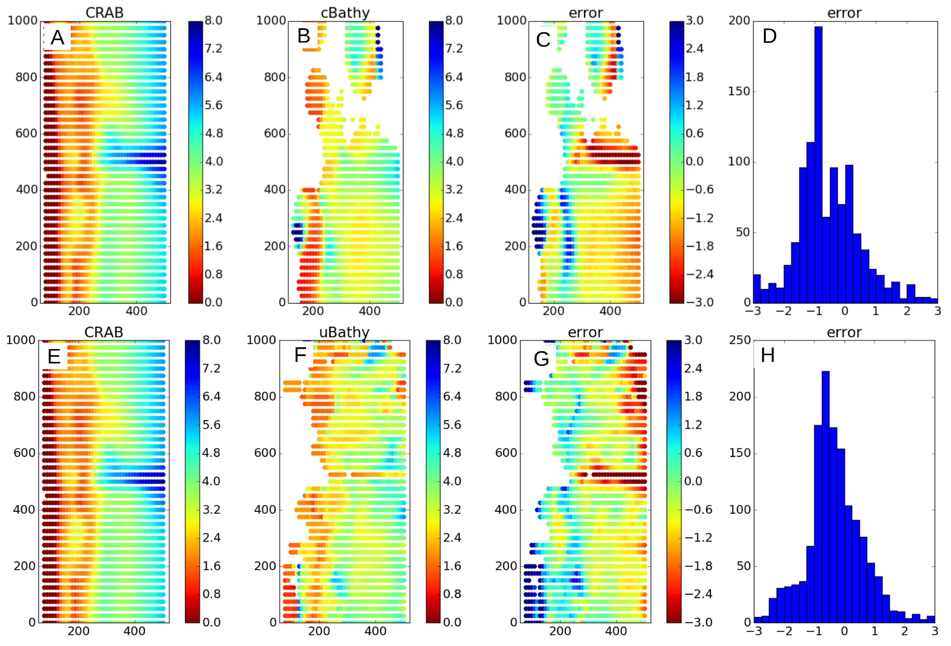
Figure 15.
On top (bottom) are results from cBathy (uBathy). From left to right: measured bathymetry with the CRAB (A,E, in m), inferred bathymetry (B,F, in m), error of the inferred bathymetry (C,G, in m), and histogram of the errors for the pixels (D,H).
Figure 15.
On top (bottom) are results from cBathy (uBathy). From left to right: measured bathymetry with the CRAB (A,E, in m), inferred bathymetry (B,F, in m), error of the inferred bathymetry (C,G, in m), and histogram of the errors for the pixels (D,H).
Table 1.
Wave conditions in the seaward boundary for the 1D examples: For each wave train (two at most), is the period, is the wave amplitude at , and is the direction of wave propagation (+, rightwards).
Table 1.
Wave conditions in the seaward boundary for the 1D examples: For each wave train (two at most), is the period, is the wave amplitude at , and is the direction of wave propagation (+, rightwards).
| Cases | | | | | | |
|---|
| monochromatic | | | + | − | − | − |
| bichromatic | | | + | | | + |
| reflective | | | + | | | − |
Table 2.
Summary of the results of the Principal Component Analysis (PCA) obtained for the 1D examples.
Table 2.
Summary of the results of the Principal Component Analysis (PCA) obtained for the 1D examples.
| | Mode | | |
|---|
| monochromatic | 1 | | |
| bichromatic | 1 | | |
| 2 | | |
| reflective | 1 | | |
Table 3.
Wave conditions in the seaward boundary for the analysis of synthetic 2D cases: For each wave train, is the period, is the wave amplitude in deep waters, is the angle with respect to the shore normal in deep waters, and is a phase lag.
Table 3.
Wave conditions in the seaward boundary for the analysis of synthetic 2D cases: For each wave train, is the period, is the wave amplitude in deep waters, is the angle with respect to the shore normal in deep waters, and is a phase lag.
| Wave Train | | | | |
|---|
| W1 | | | | |
| W2 | | | | |
| W3 | | | | |
Table 4.
Relative errors for , (in %), as a function of and for , corresponding to linear propagation of W1.
Table 4.
Relative errors for , (in %), as a function of and for , corresponding to linear propagation of W1.
| |
|---|
| | | |
|---|
| | | — | — |
| | | | — |
| | | | |
| | | | |
Table 5.
Relative RMSE for k, (in %) for , as a function of and for and corresponding to linear propagation of W1.
Table 5.
Relative RMSE for k, (in %) for , as a function of and for and corresponding to linear propagation of W1.
| |
|---|
| 1 | 2 | 4 | 10 |
|---|
| 2 | | | — | — |
| 4 | | | | — |
| 8 | | | | — |
| 12 | | | | |
| 16 | | | | |
Table 6.
Summary of the results of the PCA obtained using phase fitting (without windowing) for linear wave propagation and , , , and : Relative RMS errors and are given for . Next to the retrieved period, the corresponding wave field is indicated.
Table 6.
Summary of the results of the PCA obtained using phase fitting (without windowing) for linear wave propagation and , , , and : Relative RMS errors and are given for . Next to the retrieved period, the corresponding wave field is indicated.
| | Mode | | | | | |
|---|
| | 1 | | (W1) | | | |
| monochromatic | 1 | | (W2) | | | |
| | 1 | | (W3) | | | |
| | 1 | | (W1) | | | |
| polychromatic | 2 | | (W2) | | | |
| | 3 | | (W3) | | | |
Table 7.
Results of the PCA obtained for nonlinear wave propagation of the monochromatic W1 case with different factors: Next to the retrieved period, the corresponding wave field is indicated (when applicable).
Table 7.
Results of the PCA obtained for nonlinear wave propagation of the monochromatic W1 case with different factors: Next to the retrieved period, the corresponding wave field is indicated (when applicable).
| Factor | Mode | | |
|---|
| 1 | | (W1) |
| 1 | | (W1) |
| 2 | | ( — ) |
| 1 | | (W1) |
| 2 | | ( — ) |
| 3 | | ( — ) |
Table 8.
Summary of the results for nonlinear wave propagation of the polychromatic WS case with different factors: Relative RMSE, , are given for . Here, “p” and “f” stand for phase and function fitting of the wavenumber. Next to the retrieved period, the corresponding wave field is indicated (when applicable).
| Factor | Mode | | | |
|---|
| |
|---|
| | 1 | | (W1) | | |
| 2 | | (W2) | | |
| | 3 | | (W3) | | |
| | 1 | | (W1) | | |
| 2 | | (W2) | | |
| | 3 | | ( — ) | — | — |
| | 1 | | (W1) | | |
| 2 | | (W2) | | |
| | 3 | | ( — ) | — | — |
Table 9.
Results for the first mode for nonlinear wave propagation of the polychromatic WS case with different factors, total video length , and window width : Relative RMSE, , is given for . Here, “p” and “f” stand for results using phase and function fitting for , respectively. The number of sub-videos are included in parentheses.
| | |
|---|
| p | f | Windowing, |
|---|
| | | | |
|---|
| | | | | (112) | (94) | (56) | (18) | (1) |
| | | | | | | | | |
| s | | | | | | | | |
| | | | | | | | | |
| | | | | (225) | (207) | (169) | (131) | (113) |
| | | | | | | | | |
| s | | | | | | | | |
| | | | | | | | | |
Table 10.
Summary of the results for the field site video analysis.
Table 10.
Summary of the results for the field site video analysis.
| | cBathy | uBathy |
|---|
| percentage of points | | |
| average error (bias) | | |
| RMS error | | |

 ,
, 


