Abstract
Accurate multispectral image segmentation is essential in remote sensing research. Traditional fuzzy clustering algorithms used to segment multispectral images have several disadvantages, including: (1) they usually only consider the pixels’ grayscale information and ignore the interaction between pixels; and, (2) they are sensitive to noise and outliers. To overcome these constraints, this study proposes a multispectral image segmentation algorithm based on fuzzy clustering combined with the Tsallis entropy and Gaussian mixture model. The algorithm uses the fuzzy Tsallis entropy as regularization item for fuzzy C-means (FCM) and improves dissimilarity measure using the negative logarithm of the Gaussian Mixture Model (GMM). The Hidden Markov Random Field (HMRF) is introduced to define prior probability of neighborhood relationship, which is used as weights of the Gaussian components. The Lagrange multiplier method is used to solve the segmentation model. To evaluate the proposed segmentation algorithm, simulated and real multispectral images were segmented using the proposed algorithm and two other algorithms for comparison (i.e., Tsallis Fuzzy C-means (TFCM), Kullback–Leibler Gaussian Fuzzy C-means (KLG-FCM)). The study found that the modified algorithm can accelerate the convergence speed, reduce the effect of noise and outliers, and accurately segment simulated images with small gray level differences with an overall accuracy of more than 98.2%. Therefore, the algorithm can be used as a feasible and effective alternative in multispectral image segmentation, particularly for those with small color differences.
1. Introduction
Image segmentation, which is a remote sensing technique dividing complex images into several continuous homogeneous regions, is fundamental in object-based image analysis [1,2,3,4]. There are three main approaches to implement segmentation, namely: threshold-based [5,6], clustering-based [7], and statistics-based [8,9] algorithms. Among them, the clustering segmentation method [10] is widely used in remote sensing applications. However, along with the improvements in remote sensing sensors, multispectral image segmentation requires more complex segmentation algorithms due to the large number of spectral bands and detail feature information [11,12,13]. Thus, research exploring new techniques in image segmentation is of great significance.
The clustering method based on the fuzzy set theory is an effective tool to deal with the uncertainty of image information, which is easy to operate and can guarantee segmentation accuracy [14]. Previous studies have proposed different algorithms for implementing the clustering-based approach. The fuzzy set has been conceived by Zadeh [15], which can exhibit the uncertainty that an individual point is similarity to all the clusters. Bezdek [16] has proposed the fuzzy clustering method based on least-squared error criterion, called the Fuzzy C-means (FCM) algorithm. In this method, the weighting exponent m has been introduced to control the extent of membership sharing between fuzzy clusters [17]. Dunn [18] has improved the FCM algorithm using the Euclidean distance to quantify the Dissimilarity Measure (DSM). The algorithm has used the fuzzy membership of pixel to clusters as weight to construct the objective function in image segmentation. The optimal segmentation of images can be obtained through minimization of the objective function and derivation of the iterative algorithms for computing the membership functions of clusters in question. Although the FCM proposed by Bezdek has become ubiquitous in image segmentation, the approach continues to have major significant disadvantages, including: having no theoretical basis on weighting exponent m selection, neglecting image pixel grayscale correlation, sensitivity to noise and outliers, and inability to fit multi-peak characteristics of a remote sensing image. In order to address these constraints, the FCM algorithm is improved mainly through two main aspects: objective function and dissimilarity measure.
With regards to the objective function, in order to overcome the lack of theoretical basis of the weighting exponent m, several improved fuzzy clustering algorithms based on the entropy theory have been proposed. For example, the Shannon entropy has been introduced into the FCM algorithm by Li et al. [19], leading to a new fuzzy clustering algorithm, wherein the minimization of the objective function is achieved using the Maximum Entropy Inference (MEI) within the context of FCM. Compared with the other FCM algorithms, this method has clear mathematical features and physical significance, which has piqued the interest of a large number of researchers. Miyamoto et al. [20] and Tran et al. [21] has introduced Shannon Entropy into the objective function of FCM using an arithmetic weighted system and proposed the Entropy FCM (EFCM) algorithm. Li K. et al. [22] has proposed the Generalized Entropy FCM (GEFCM) algorithm based on the Generalized Entropy, utilizing the adjustment of two parameters that would achieve better segmentation results, which has resulted in challenges in finding the optimal solution. Liao S. et al. [23] has introduced the fuzzy entropy that redefined the objective function. In this algorithm, the membership function is affected not only by distance measure but also by the fuzzy entropy, which reduces the adverse effects of noise and outliers in the cluster centers and drives the clustering results to become more objective.
All the aforementioned algorithms make the Shannon entropy as the entropy regularization term in the objective function to achieve the optimal effect of the FCM. However, the usage of the Shannon entropy is significantly limited, given its inability to consider the influence of cluster size and cluster correlation on segmentation results [24]. When the cluster scale is largely different (clusters with large pixel values coexisting with other clusters with small number of pixels), the algorithm can easily segment the edge pixels of the larger-scale cluster into the smaller-scale cluster. Afterward, the Tsallis entropy has been proposed to measure the nonextensivity of the physical system, which uses an exponential weighted form of entropy to describe the interrelation between subsystems [25,26,27]. Over the years, the Tsallis entropy has become widely used in image segmentation due to its universality. As the generalized form of the Shannon entropy, the Tsallis entropy could describe the correlation described by the nonextensive parameter q between the grayscale value of pixels in images. Image segmentation methods based on the Tsallis entropy considered the interaction between clusters, which is favorable in segmenting images with nonextensive features [28,29,30,31,32]. Among them, a new multilevel thresholding technique based on the Tsallis entropy for colored satellite image has been proposed, achieving segmentation of complex images with small color differences and having the ability to describe the interrelationship between clusters [28]. Kaur et al. have proposed a hybrid multilevel thresholding technique that combines intuitionistic fuzzy sets and Tsallis entropy for the automatic delineation of tumors in magnetic resonance images with vague boundaries and poor contrast [29]. However, both techniques that applied the fuzzy Tsallis entropy to threshold segmentation still suffer a major limitation, as they can only segment one-dimensional images. In order to describe the long-range interaction between grayscale values of color image, Yasuda [33] has maximized the Tsallis entropy within the FCM framework and made a quantitative description of the relationship between the nonextensive parameter (q) and temperature through the Deterministic Annealing (DA) method. Although this method explains the tangible implications of maximizing Tsallis entropy from a mathematical perspective in detail, it undermines the role of FCM and makes the solution process more complex.
Aside from refining the objective function, a number of researchers have examined the dissimilarity measure based on the distance function and probability distribution model to improve further the accuracy of the fuzzy clustering algorithm. Most traditional fuzzy clustering algorithms used the cluster center to represent the cluster, and the dissimilarity measure has usually been defined by the Euclidean distance between the pixel and the cluster center [16,17]. However, the dissimilarity measure based on the Euclidean distance fails to accurately distinguish the clusters with non-spherical distribution and cannot effectively segment detail information. The traditional fuzzy clustering segmentation algorithm based on the Euclidean measure is sensitive to noise and outliers, and the segmentation results are easily affected by the shape, density, and size of clusters (i.e., pixel distribution in feature space and the number of pixels in homogeneous regions). In addition, the algorithm has an extreme dependence on the initial cluster center, and thus cannot effectively be used for multispectral remote sensing image segmentation. Other scholars have used the Mahalanobis distance to consider the influence of clustering variance on dissimilarity measure, which can more effectively distinguish clusters with varying shapes and scales [34,35]. However, it is still expressed using the cluster center, which can reduce the resulting accuracy.
To better describe the cluster, some researchers have used probability distribution to define the dissimilarity measure of the fuzzy clustering algorithm [36,37,38], which can compensate, to some extent, for the shortcomings of distance dissimilarity measure. The factor probability distribution clustering (FPDC) method uses the Tucker3 decomposition to perform linear transformation and assigns pixels to clusters based on the probability that they belong to a given cluster [36]. This probability distribution clustering performs well when the clusters are elliptically shaped, but it becomes unstable when the number of variables is large, and the variables are correlated. Chen et al. have proposed a probabilistic distance function based on kernel density estimation for categorical attributes [37].
With gradual improvements in their spatial resolution, recent remote sensing images generally have multipeak characteristics, and their distribution characteristics become more complex. In order to describe the multi-peak distribution characteristics more accurately, the Mixture Model (MM) has been developed to create an image segmentation model [39,40]. For example, agglomerative clustering, based on combinations of non-Gaussian distributions, has been developed for statistical-based image segmentation [41]. This method adopts higher-order statistics in pixel distributions instead of second-order statistics as correlation. It appends non-Gaussian mixture models estimated for every clustering building with a hierarchical structure by using Kullback–Leibler divergence. Although agglomerative clustering performs well in segmenting regions of images in similar areas, varying levels of dependence of the variables increase the complexity of the algorithm. Because of its simple structure and the fact that most remote sensing images have Gaussian characteristics, the Gaussian Mixture Model (GMM), which is a mathematical technique fitting complex distribution through a set of simple density distribution weighted combination, have been proposed to fit the multipeak distribution feature data of remote sensing images [42,43].
Traditional FCM is sensitive to noise and outliers, and do not consider the gray information of image pixels. Also, the results are easily influenced by shape, density, and size of the clusters. To address these limitations, we developed the fuzzy clustering algorithm combined with the Tsallis entropy and the Gaussian mixture model (TGMM-FCM) as an alternative approach to image segmentation. The fuzzy Tsallis entropy is introduced into FCM as a regular term to define an improved objective function. Compared with the traditional objective function, this objective function not only considers the image pixel gray information but also considers the pixel distribution characteristics (i.e., the correlation degree between gray levels). The GMM is then used to represent clusters that can accurately fit the multi-peak features of remote sensing images. The labeling field is established with the Hidden Markov Random Field (HMRF) [44,45], and is used to characterize the prior probability of the neighborhood spatial relationship to effectively eliminate noise effects. The spatial function between neighborhood pixels based on the labeling field is designated as the prior probability of image pixels, and the prior probability is taken as the weight of GMM components to be used in constructing GMM dissimilarity measure.
The remainder of this paper is organized as follows: in Section 2, the proposed methodology is succinctly discussed. This section also describes image segmentation evaluation methods and optimization techniques employed in this study and quantitatively measures the effective value range of the nonextensive parameter q. In Section 3, the results from the segmentation experiments of simulation and multispectral images are presented. The qualitative and quantitative evaluation of accuracy is discussed, which is then related to the effectivity analysis of the TGMM-FCM algorithm. Finally, Section 4 presents the study’s conclusions.
2. Methodology
2.1. Overview
This paper proposes the Fuzzy Tsallis Entropy-Clustering Algorithm Combined with Gaussian Mixture Model (TGMM-FCM). The framework of the proposed algorithm is presented in Figure 1. The key concepts include the adoption of the fuzzy Tsallis entropy to describe the correlation between pixel grayscale and the use of the Gaussian Mixture Model (GMM) for fitting the multi-peak features. This method is employed to develop an efficient procedure for multispectral remote sensing image segmentation, which would be able to overcome the shortcomings of traditional FCM and improve the segmentation accuracy of multispectral images.
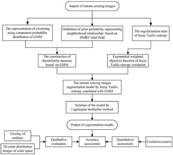
Figure 1.
The framework of the fuzzy clustering algorithm combined with the Tsallis entropy and the Gaussian mixture model (TGMM-FCM).
2.2. Fuzzy Tsallis Entropy-Clustering Segmentation Model
Let X = {x1, x2, …, xi, …, xN} be the remote sensing images of p dimensions, where xi = (xi1, xi2, …, xip)T is the spectral measure vector of ith pixel, and N is the number of image pixels. The images can be divided into c homogeneous regions (i.e., clusters) by a fuzzy clustering algorithm. Let {Xj: 1 ≤ j ≤ c} ⊂ F(X), such that F(X) represents the division of image X. Let U = [uij]N×c be the fuzzy membership matrix to characterize the fuzzy segmentation of image, where the fuzzy membership function uij is used to describe the membership of the pixel i to the clustering j. In order to determine the optimal U, we need to perform the following: (1) define the dissimilarity measure of pixels and clustering; (2) structure the objective function by this measure; and, (3) obtain the optimal fuzzy segmentation result by minimizing the objective function.
The Shannon entropy satisfies the additivity criterion, assuming the systems or pixels are independent of each other. However, the idealized model does not perform adequately with complex images since it cannot describe the interaction between pixels of an image. Tsallis [25,26,27] has introduced the nonextensive parameter q based on the Shannon entropy and proposed a type of nonextensive entropy, which works well in describing the thermodynamic properties of nonextensive physical systems:
where, q {q > 0 | q ≠ 1} is an index used to describe the nonextensive extent. When q approaches 1, the Tsallis entropy and Shannon entropy become equivalent. When Pj approaches 1/c, the Tsallis entropy and Reny entropy become equal. When 0 < q < 1 and Pjq > Pj, the small probability events are increased, while the big probability events are suppressed. When q > 1 and Pjq < Pj, the small probability events are suppressed, while the big probability events are intensified. The best value range of q is [0.8, 1.5] [46].
As article [47] said, the Tsallis entropy, a kind of generalized entropy, can both sufficiently characterize the cluster-to-cluster interactions and be used for the quantification of nonextensive images. According to the definition of the fuzzy entropy [31,48], the Tsallis entropy can accurately be defined as the expected value of fuzzy membership [33], which is called the Fuzzy Tsallis Entropy Function E(U), to present the average fuzzy extent of images:
The fuzzy Tsallis entropy function has been proven to satisfy the following conditions: (1) When uij = 1/c, the E(U) will reach the maximum value, and decreases as uij moves closer to 0 or 1. (2) As for the independent fuzzy sets, E(U) satisfies the pseudo-additive criterion. The fuzzy Tsallis entropy can describe the average uncertainty (ambiguity) of fuzzy sets, which is often used as an indicator of cluster validity. The smaller the value of E(U), the smaller the average uncertainty of the fuzzy set is, which produces clearer segmentation results.
The TGMM-FCM is an improved algorithm based on the Fuzzy Entropy-Clustering (FEC). The objective function of FEC is defined as the difference between the objective function of the Hard C-means (HCM) and the fuzzy Shannon entropy multiplied by a fuzzy factor [21]. The minimization process of the objective function can simultaneously satisfy the requirements of the minimum distance and the maximum fuzzy entropy function, in order to obtain the optimal division. In this study, we define the objective function of the new model as the difference between the FCM’s objective function and the fuzzy Tsallis entropy:
where i is the pixel index, j is the clustering index, N is the total number of image pixels, c is the number of clusters, dij is the dissimilarity measure from ith pixel to jth center of clustering, and uij is the membership of the pixel i to the clustering j. The E(U), as the fuzzy Tsallis entropy regularization term, can improve the smoothing of the improved fuzzy algorithm [33]. It can also describe the interaction of the pixels’ gray values to better segment images with only small grayscale differences.
2.3. GMM Dissimilarity Measure
Based on their statistical attributes, most remote sensing data can be characterized by a Gaussian distribution. Thus, in this study, the dissimilarity measure of pixels to clusters is established with the use of the GMM. The mean vector and covariance matrix can be calculated using the GMM dissimilarity measure, and the statistical distribution can be fitted with high precision. Suppose that pixels belonging to the same homogeneous region are subject to the same Gaussian probability distribution, i.e., P(xi | vj, Σj), determined by the mean vj and covariance Σj of clusters. In the image segmentation, every pixel can belong to each cluster due to the fuzziness. In this paper, the prior probability from the HMRF is used as weight of the mixture model, and the Gaussian probability distribution is used as the component function of GMM. The formula of the Gaussian Mixture Model P(xi | wi, v, Σ) is:
where,
For computational convenience, the dissimilarity measure dij can be defined as the negative logarithm of the jth, component in the GMM:
Combining Equation (5) and Equation (6), the dissimilarity measure dij of the ith pixel to jth cluster can be written as:
where, wi = {wij; j = 1, 2, …, c} is the prior probability vector, such that each element wij is the prior probability of ith pixel to jth cluster; v = {vj; j = 1, 2, …, c} is the mean cluster vector set, such that each element vj is the mean vector of jth cluster; Σ = {Σj; j = 1, 2, …, c} is a set of covariance matrix, such that each element Σj is the covariance matrix of cluster j; and, p is the number of bands of remote sensing images. The dissimilarity measure expressed in Equation (7) can reconcile the contributions of the different bands to the segmentation results, and can effectively use the spectrum information of the different bands to improve the segmentation accuracy of remote sensing images.
2.4. Label Field Model
In order to introduce the special relationship of pixels into the dissimilarity measure, w = {wij; i = 1, 2, …, c, j = 1, 2, …, n} is defined by the Hidden Markov Random Field (HMRF) function that can characterize the neighborhood relation. The prior probability wij presents the role of the neighborhood pixels with the same label as the central pixel. In general, compared with the non-neighborhood pixels, the neighborhood pixels are more likely to have the same label. Thus, the introduction of the prior probability based on neighborhood relationship can effectively avoid segmentation errors from noise.
In this study, the label field is modeled by the HMRF. Assume that L = (l1, l2, …, lN) is the label field of a given image X, where li∈{1, 2, …, c} is the label of the ith pixel. The maximum membership criterion is adopted to realize defuzzification, and pixel label is determined:
where li represents the cluster where pixel i belongs (implementation of the label of pixel i). This means that the label of the cluster corresponding to the maximum fuzzy membership of the pixel i is assigned to the label field.
In the label field, the potential energy function Vc is established as follows:
where i′ is the neighborhood pixel index of pixel i, and li′ is the label of the neighborhood pixel index. When the neighborhood pixel has the same label as the central pixel, it reaches a steady-state with a potential energy of 0; otherwise, the potential energy is 1.
In constructing the prior probability, a 3 × 3 pixel-square neighborhood window around pixel i is referred to as the eight-neighborhood pixel set, as shown in Figure 2a. As example, Figure 2b presents a label field implementation of pixel i’s neighborhood window. In this label field, the neighborhood potential energy distributions of the central pixel with different labels are shown in Figure 2c–e. When the label of the central pixel is 1, the potential energy corresponding to its neighborhood is lowest.
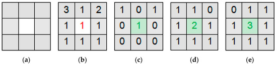
Figure 2.
Procedure used in defining the relationship between potential energy and label field. (a) Eight-neighborhood window; (b) The label field; (c) The neighborhood potential energy distribution when li = 1; (d) The neighborhood potential energy distribution when li = 2; (e) The neighborhood potential energy distribution when li = 3.
The prior probability is defined as the e index of the sum of the negative potential energy functions. In order to increase the corresponding prior probability of low potential energy state, the probability is normalized to satisfy the constraint condition . Then, the prior probability of the pixel i belonging to cluster j is estimated by:
where b is a parameter representing the label interaction intensity of the neighborhood, with values ranging from any real number between [0, 1]. The larger the b value, the more the central pixel is affected by its neighborhood, which is suitable for images with more noise. Smaller b values indicate smaller neighborhood effects, which is suitable for images with more detailed information or more linear features.
2.5. Solution of Segmentation Model
In order to obtain the optimal fuzzy segmentation, the objective function is minimized by calculating the partial derivatives of each parameter and making the partial derivatives to be zero. Since the constraint of uij is , the Lagrange multiplier βi is introduced into the objective function of Equation (3) to construct the Lagrange equation:
The partial derivative of Equation (11) is determined and taken to be equal to zero, such that:
where, m is the fuzzy factor to describe the fuzzy extent of the pixel i belonging to cluster j, and q is the nonextensive parameter to represent the nonextensive degree of image. A large m-value indicates a large fuzzy extent, while an m-value close to one suggests a small fuzzy extent. According to Equation (12), the condition where m > q and m < q is similar to the mathematical phenomenon of large number + decimal, such that the influence of the decimal part in Equation (11) becomes negligible. Therefore, only when m = q can the exponentially weighted measure term and the fuzzy Tsallis entropy term in Equation (11) both impact the objective function simultaneously. In the image segmentation application, the fuzzy factor and the nonextensive parameter in Equation (3) can be uniformly represented by q, and the Equation (3) can be rewritten as:
When the GMM dissimilarity measure is introduced into the Equation (13), expression becomes:
where, q has a dual physical meaning, which can represent the degree of ambiguity in the algorithm and can also describe the nonextensive parameters in statistics. The value of q directly controls the quality of the segmentation results, so we can select it according to the statistical characteristics of the images (the variance and mean of the clusters). The value of q is selected from the range of (0, 1) to segment images with small noise and highly detailed information, which has the effect of enlarging small differences. The value of q is selected from the range of (1, ∞) to segment images with more noise and continuous regions, which can effectively remove spot noise. The fuzzy Tsallis entropy provides the statistical characteristics of the images, which can be used to describe the average fuzziness of the image and the correlation between the gray levels of the pixels.
According to the Lagrange multiplier method, the membership degree uij, the cluster center vj and the covariance matrix Σj are expressed as follows:
In summary, the specific steps of implementing the proposed algorithm are as follows:
Step 1: Set the constants, including: the number of cluster c, nonextensive parameter q, neighborhood interaction intensity b, terminal condition Ɛ, and the total iterations. Also, set the initial U(0).
Step 2: Solve the label field according to Equation (8).
Step 3: Compute the cluster center vj(z) of jth cluster using Equation (16).
Step 4: Solve the covariance matrix Σj(z) of jth cluster according to Equation (17).
Step 5: Compute the prior probability wij(z) combined with the label field using Equation (9) and Equation (10).
Step 6: Substitute wij(z), vj(z), and Σj(z) into the Equation (7) to calculate the dissimilarity measure dij(z).
Step 7: Update the membership degree uij(z+1) of the ith pixel belonging to the jth cluster by using Equation (15).
Step 8: Evaluate the condition whether ||U(z+1)-U(z)|| < Ɛ. Upon confirmation that the mathematical statement is true, the iteration process is stopped, and the defuzzification is performed based on the final membership matrix. Otherwise, the second step is iterated.
2.6. Quantitative Analysis of q
In order to quantitatively analyze the effective value range of the nonextensive parameter q in the TGMM-FCM algorithm, we use the Fuzzy Tsallis Entropy-Clustering Algorithm (T-FCM) with the Euclidean distance and Fuzzy Entropy-Clustering (FEC) algorithm [21] to segment the test image with 128 × 128 sized pixels, as shown in Figure 3. In Table 1, the records of the objective function value (Jq) and convergence time (t) of TFCM under different parameters (q) are tabulated, as well as the objective function value (Jm) and convergence time (t) of FEC under different fuzzy factors (m).
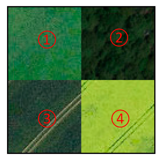
Figure 3.
Test image.

Table 1.
Comparison of clustering results with different parameters of each algorithm.
When evaluating Table 1 and Figure 4a, the FEC is seen to be unaffected by changes in m when m < 1, suggesting that the algorithm fails at this condition. Theoretically, this is consistent with the fact that the fuzzy factor should be greater than one. When m > 1, the objective function value produces small fluctuations with changes in the fuzzy factor, which means that the FEC algorithm is stable, and the value of the fuzzy factor has little effect on segmentation results. In Figure 4a, as the blue line indicates, the objective function value of T-FCM undergoes an abrupt change when the q is equal to 1.1 and then falls steadily with increasing q at the range of [1.1, 2.25]. Past the q value of 2.25, the T-FCM experiences large fluctuations with small changes in q. Thus, the effective range of q for image segmentation using T-FCM is [1.1, 2.25], and the selection of nonextensive parameters (q) can significantly influence the segmentation results.
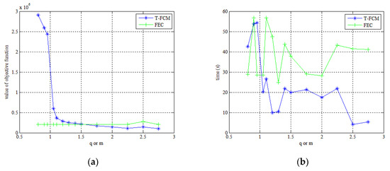
Figure 4.
(a) The objective function value curve of the Fuzzy Tsallis Entropy-Clustering Algorithm (T-FCM) / Fuzzy Entropy-Clustering algorithm (FEC) varying with the parameter q/fuzzy factor m. (b) the time curve of TFCM/FEC algorithm varying with the parameter q/fuzzy factor m.
From Figure 4b, the convergence time t required for segmentation with T-FCM is clearly smaller than the alternative algorithm. Because the Tsallis entropy is in the exponential form, the change is more pronounced, while the Shannon entropy is in the logarithmic form, such that the change is more gradual. Thus, the fuzzy Tsallis entropy has the advantage of high efficiency compared with the fuzzy Shannon entropy, which can reduce the temporal redundancy to some extent.
3. Experimental Result and Discussion
In this study, the operating environment was a personal computer with 4G memory and an intel(R) i5 3rd generation processor. MATLAB programming was used in performing the segmentation experiments of multispectral images. To examine the feasibility and effectiveness of the algorithm, two other algorithms were used for comparison: the T-FCM and the Kullback–Leibler Gaussian Fuzzy C-means (KLG-FCM). The KLG-FCM adopts the negative logarithm of the Gaussian Distribution Function as the dissimilarity measure and uses the Kullback–Leibler (KL) divergence information as the regularization term of the objective function, achieving the fuzzification of objective function and representing the neighboring relationship with HMRF [49,50]. In the experiment, the different algorithms were used to segment the simulation images and multispectral images. Qualitative and quantitative evaluation of segmentation accuracy was employed to analyze the effectiveness of the TGMM-FCM algorithm.
3.1. Simulation Image Segmentation
Figure 5b is a simulation image generated according to a template image (shown in Figure 5a) at 128 × 128 pixel size. The template image has five unequal-sized homogeneous regions of irregular shapes, with the hexagonal shape (region (3)) accounting for the largest area. Figure 5b displays different scenes taken from IKONOS at a four-meter spatial resolution. As shown in Table 2, some regions of the simulation image have small differences in mean, but all the homogeneous regions have significant variances.
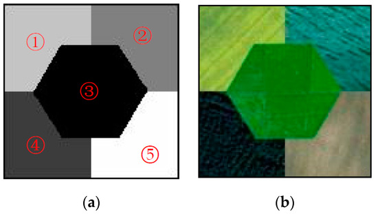
Figure 5.
Template image and simulation image. (a) presents template image at 128 × 128 pixel size; (b) presents simulation image with different scenes taken from IKONOS at a four-meter spatial resolution.
Table 2.
Mean and variance of simulation image.
Figure 6 shows the segmentation results and contour overlays obtained by segmenting the simulation image using T-FCM, KLG-FCM, and the proposed algorithm. Figure 6(b1) shows that the T-FCM algorithm is able to execute the segmentation for regions (1) and (3) with similar cluster mean values, while the segmentation for regions (2) and (4) is not ideal where the texture features were more complicated. In Figure 6(b2), because the KLG-FCM algorithm introduced neighborhoods, the internal regions are smooth and continuous. However, since the Gaussian distribution, as the dissimilarity measure, can only solve the characteristics independently, the boundaries became blurred, and the segmentation effect is not ideal. In Figure 6(a3), the internal regions are smooth and continuous without error pixels, and the outlines are clear and linear with few jagged lines. The GMM dissimilarity measure in this algorithm appears to accurately fit the statistical features of each region in the image and has satisfactory performance in segmentation of images with similar means of the interregion and significant variances of the intraregion.
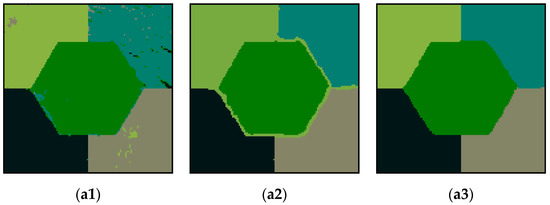
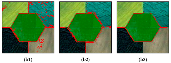
Figure 6.
Segmentation results of each algorithm and overlay of outlines. (a1) presents the segmentation results obtained using the TFCM algorithm when the nonextensive parameter q takes a value of 1.9. (b1) displays the outline overlaid on the segmentation results obtained from the TFCM algorithm. (a2) presents the segmentation result obtained using the KLG-FCM algorithm when b = 0.2, m = 1.1. (b2) displays the outline superimposed on the segmentation results obtained from the KLG-FCM algorithm. (a3) displays the segmentation result obtained using the proposed algorithm when b = 0.2, q = 1.3. (b3) presents the outline overlaid on the segmentation results obtained from the TGMM-FCM algorithm.
To explain how the TGMM-FCM algorithm compares with other algorithms in terms of how it can accurately fit the data distribution characteristics, we analyzed the segmentation results of each algorithm from a microscopic perspective. The 3D distribution of segmentation results using the T-FCM (shown in Figure 7b) indicates that the points belonging to the region and distant from the cluster center are easily segmented by mistake. The 3D distribution of segmentation results by KLG-FCM is shown in Figure 7c. In Figure 7c, the Gaussian distribution dissimilarity measure could completely match the statistical properties of regions (2), (4) and (5); but since the correlation between regions is neglected, the pixels belonging to region (3) are segmented into region (1). In Figure 7d, the TGMM-FCM algorithm assigns the GMM with weights characterizing the neighborhood relationship to each pixel. The color space distribution of each region could be restored in the original image by accurately fitting the statistical features of each region and allocating remote discrete points into the correct clusters. Based on the experimental results, the proposed algorithm is able to successfully segment the complex images accurately.
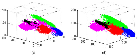
Figure 7.
3D point distribution images of color space of simulation image and segmentation results by the TFCM, KLG-FCM, and TGMM-FCM, where three axes represent the spectral bands of red, green, and blue. The pink rhombus ‘◆’, black square ‘□’, green asterisk ‘*’, blue circle ‘○’ and red plus ‘+’ denote the pixel spectral measure and their distribution in clusters (1), (2), (3), (4), and (5), respectively. (a) presents 3D point distribution images of color space of simulation image; (b) presents 3D point distribution images of color space of segmentation results by the T-FCM; (c) presents 3D point distribution images of color space of segmentation results by the KLG-FCM; (d) presents 3D point distribution images of color space of segmentation results by the TGMM-FCM.
In order to verify the robustness and anti-noise of the TGMM-FCM algorithm, another set of simulation images, in which the spectral measure of each pixel follows a consolidated Gaussian distribution, is constructed following the method as proposed by Bioucas-Dias et al. [51]. Figure 8b is the simulation image generated according to the template image (shown in Figure 8a) at 256 × 256 pixel size. The template image has five homogeneous regions with regular shapes. The pixels of homogeneous region follow the same Gaussian mixture distribution as shown in Table 3. As shown in Figure 8c,d, some Gaussian noise is added into the initial simulation image to form new simulation images with different signal-to-noise ratio (SNR).
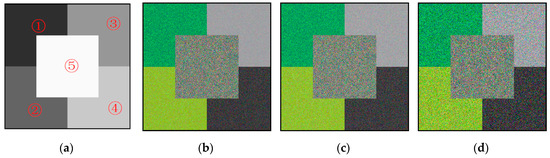
Figure 8.
(a) presents the template image; (b) shows the simulation image; (c) presents the simulation images with SNR (signal-to-noise ratio) = 20; (d) presents the simulation images with SNR =10.
Table 3.
Mean and variance of the simulation image.
The T-FCM, KLG-FCM, and the proposed algorithms were used in this section to segment the simulation images with different SNR, to verify the anti-noise performance of the TGMM-FCM proposed in this study. The segmentation results and contour overlays are shown in Figure 9. In Figure 9(a1–a4), the quality of the segmentation results obtained by the T-FCM is inferior, because the Euclidean distance cannot adequately recognize probability distributions of interregions. In Figure 9(b1–b4), the segmentation results of the KLG-FCM are better than the T-FCM due to the neighborhood and the Gaussian dissimilarity measure. However, many pixels have been erroneously grouped in regions (2) and (5), with large variance of intraregion and small difference in interregion means. Noise content has significant influence on the segmentation result in the T-FCM and KLG-FCM. As shown in Figure 9(c1–c4), the internal regions are smooth and continuous without error pixels, and the outlines are clear-cut and smooth with few jagged lines. And the segmentation results of TGMM-FCM are scantily influenced by noise.
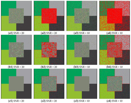
Figure 9.
Segmentation results of simulation images with different SNR obtained by each algorithm and the overlay of outlines. (a1) presents the segmentation result of the simulation image with SNR = 20 obtained using the T-FCM algorithm when the nonextensive parameter q takes a value of 1.1; (a2) displays the outline overlay image of (a1); (a3) presents the segmentation result of the simulation image with SRN = 10 obtained by the T-FCM algorithm when q = 1.1; (a4) is the overlay image between original image and the outline of segmentation result (a3); (b1) is the segmentation result of the simulation image with SNR = 20 using the KLG-FCM algorithm when b = 0.5 and m = 1.1; (b2) is the overlay image of the contour of (b1); (b3) shows the segmentation result of the simulation image with SNR = 10 segmented by the KLG-FCM algorithm when parameters are b = 0.3 and m = 1.05; (b4) presents the contour overlay image of (b3); (c1) displays the segmentation result of simulation image with SNR = 10 by TGMM-FCM when b = 0.8 and q = 1.1; (c2) is the overlay image between the contour of (c1) and the origin image; (c3) displays the segmentation result of the simulation image with SNR = 10 obtained from the proposed algorithm when b = 0.9 and q = 1.05. (c4) presents the outline overlay image on the segmentation results obtained from the TGMM-FCM algorithm.
In order to quantitatively evaluate the accuracy of the segmentation results, the template images in Figure 5a and Figure 8a were used as the criterion to calculate the confusion matrix generated by the segmentation results (shown in Figure 6 and Figure 9). The product accuracy, user accuracy, overall accuracy, and Kappa value were calculated according to the confusion matrix, as shown in Table 4 [52]. Indices with larger values correspond to higher accuracy segmentation, while accuracy often suffers from imbalanced data sets. Balanced accuracy (BACC) overcomes this problem by normalizing true positive and true negative predictions with the use of the number of positive and negative samples, respectively [53]. As presented in Table 4, the balanced accuracy was calculated using the confusion matrix. The overall accuracy using the T-FCM algorithm is less than 95.65%, and the Kappa value is less than 0.95. For the T-FCM algorithm, the product accuracy in region (5) of the simulation image with SNR = 10 is less than 50%, while the user accuracy is lower than 70%. As shown by the results, the performance of the T-FCM algorithm is worse with the presence of more noise. Compared with the T-FCM, the KLG-FCM algorithm has higher accuracy, but the product accuracy in region (5) of the simulation image with large noise is still less than 80%. The BACC demonstrates that KLG-FCM is also influenced by noise. For the TGMM-FCM algorithm, the overall accuracy is more than 98.20%, and the Kappa value and BBCC are more than 0.98, which are higher than the other algorithms. The balanced accuracy of simulation images with different SNR are all close to 100%. This means that TGMM-FCM algorithm has higher segmentation accuracy than the other algorithms, is suitable for segmenting complex images accurately and efficiently, and has satisfactory anti-noise performance.
Table 4.
Segmentation results’ accuracy of simulation images.
3.2. Multispectral Image Segmentation
To verify the segmentation effect in actual multispectral images, we used the three algorithms in segmenting four sets of four-band (red, green, blue, and near-infrared) multispectral remote sensing images (as shown in Figure 10). The images are displayed in natural color composite (Figure 10a–d) and in near-infrared gray images (Figure 10e–h). In Figure 10a,e, the delineation of seawater and forest is complicated, given that their mean values are similar in the natural-color image, while the demarcation in the near-infrared image is recognizable and distinct given the unique spectral reflectance curve of vegetation. In Figure 10b,f, the infrastructure in the area contains a number of overpasses, which appears as long and narrow features. In the background, two types of features with small differences in gray level are presented, which would entail higher requirements in the algorithm. In Figure 10c,g, given that the pathways in this area are few, they could easily be omitted during segmentation. Moreover, the other three homogeneous regions are covered by different types of vegetation with similar spectral characteristic curves, so the difference in the near-infrared images is small. In Figure 10d, the color of sandy soil and asphalt road is similar, which is hard to distinguish visually and challenging to segment.
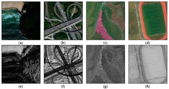
Figure 10.
Multispectral remote sensing images. (a) & (e) present near-infrared multispectral images with spatial resolution of 1.24 m from the WorldView-3 optical satellite and size of 128 × 128 pixels, including three kinds of features: beach, sea, and forest. (b) & (f) show near-infrared multispectral images derived from the China Gaofen-2 optical remote sensing satellite with spatial resolution of 4 m and size of 128 × 128 pixels, including three types of features: lakes (highlighted by red box), vegetation, and transportation infrastructure. (c) & (g) are also near-infrared multispectral images derived from Gaofen-2 remote sensing satellite with spatial resolution of 4 m and size of 256 × 256 pixels, in which four features are classified as flower nursery-1, flower nursery-2, lawn, and pathway respectively. (d) & (h) present near-infrared multispectral images with spatial resolution of 4 m from Gaofen-2 optical remote sensing satellite and size of 200 × 200 pixels, including four kinds of features: rubber track, sandy soil, lawn and asphalt road.
As shown in Figure 11(a1), the waves and seawater have obvious color differences. Since the T-FCM algorithm distinguishes dissimilarity using Euclidean distance, each band has the same contribution to the segmentation results. Therefore, a number of pixels that should belong to seawater are grouped together with the beach (see Figure 11(a1)). In Figure 11(a2), the shape of the overpass is roughly delineated, with very apparent discontinuities. In addition, the T-FCM algorithm grouped shaded parts of the overpass together with the lake. From the contour overlay in Figure 11(b2), there are a large number of discrete spots in the segmentation result. In Figure 11(a3), the flower nursery-1 is completely divided, but the pathways and some parts of the lawn are erroneously apportioned into the flower nursery-2. From the delineated overlay image in Figure 11(b3), the segmentation result of the whole area is not continuous. In Figure 11(a4), a small portion of the lawn is assigned to the sandy soil region. Based on Figure 11(b4), the segmentation result roughly describes the distribution of features in the original image.
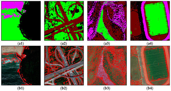
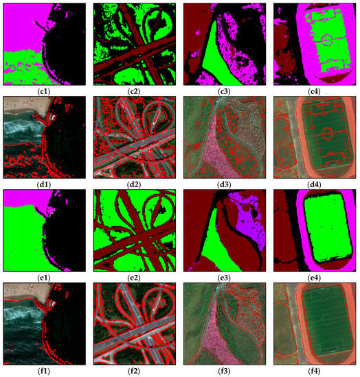
Figure 11.
Segmentation results of algorithms and overlay of outlines. (a1) shows the segmentation result of TFCM when q = 1.5; (a2) shows the segmentation result of TFCM when q = 2.25; (a3) shows the segmentation result of TFCM when q = 1.4; (a4) shows the segmentation result of TFCM when q = 1.1; (b1)–(b4) are outlined overlay images of the TFCM segmentation results and the original multispectral images; (c1) shows the segmentation result obtained using the KLG-FCM algorithm with b = 0.6 and m = 1.1; (c2) shows the segmentation result from the KLG-FCM algorithm at b = 0.05 and m = 0.9; (c3) shows the segmentation result from the KLG-FCM algorithm at b = 0.2 and m = 1.1; (c3) shows the segmentation result from the KLG-FCM algorithm at b = 0.4 and m = 1.1; (d1)–(d4) are corresponding outlined overlay images of KLG-FCM; (e1)–(e4) are the segmentation results of the TGMM-FCM algorithm; (f1)–(f4) are corresponding outlined overlay images of TGMM-FCM.
In Figure 11(c1), even when combined with the neighborhood effect, parts of the wave are still combined with the beach. In Figure 11(c2), the narrow overpass and water are grouped in the same area. There are many misappropriated pixels in the upper left vegetation area, as shown in Figure 11(d2). In Figure 11(c3,d3), only the flower nursery-1 is completely segmented, while the other parts of the image are segmented by mistake. As shown in Figure 11(c4,d4), the segmentation result of the sandy soil is incomplete, and the bright part of lawn is mistakenly segmented into the rubber track.
Figure 11(e1) shows the segmentation results obtained using the TGMM-FCM algorithm with b = 0.7 and q = 1.1. The fuzzy Tsallis entropy can better characterize the spatial correlation between grayscales by adjusting the nonextensive parameter q. The GMM dissimilarity measure can accurately get the mean feature and covariance feature of each region, while the prior probability characterizing the neighborhood effect to be used as the weight of the Gaussian component, can further remove noise effects on the segmentation results. In Figure 11(f1), TGMM-FCM is able to neutralize the brightness change in seawater and accurately divide the seawater region. Figure 11(e2) shows the segmentation result obtained by the TGMM-FCM algorithm at b = 0.05 and q = 1.1. The transport infrastructure is correctly segmented, while the vegetation region showed few erroneously partitioned pixels. Figure 11(e3) shows the segmentation result obtained by the TGMM-FCM algorithm when b = 0.2 and q = 1.2. In this segmentation result, the flower nursery-1, nursery-2, and lawn are completely partitioned. Figure 11(e4) shows the segmentation results obtained by TGMM-FCM algorithm when b = 0.5 and q = 1.1. The result shows that each region is smooth and continuous with good segmentation effect. Simply put, the algorithm can segment remote sensing images with large regional correlation, and the segmentation results would be generally acceptable.
4. Conclusions
In this study, a fuzzy Tsallis entropy-clustering algorithm combined with GMM was proposed. The proposed algorithm utilizes the fuzzy entropy form to fuzzify the Tsallis entropy, defines the fuzzy Tsallis entropy function based on fuzzy membership, and then uses the fuzzy Tsallis entropy as regularization item. The objective function is defined as the difference between the objective function of FCM and the fuzzy Tsallis entropy. Based on mathematical analysis, the fuzzy factor and the nonextensive parameter in the objective function are combined, and the nonextensive parameter q is used to describe the fuzzy degree and nonextensive characteristics of the image. Additionally, the image label field is defined using the HMRF. Prior probability of center pixel with the eight-neighborhood system is computed as the weight of the GMM component to characterize information from neighboring pixels. The dissimilarity measure is defined in the negative logarithmic form.
The experimental results showed that the nonextensive parameter q directly affects image segmentation, and its effective range is from 1.1 to 2.25. The value of q can be adjusted with image statistical features to achieve the ideal segmentation results. Using the proposed algorithm and two other algorithms for comparison, segmentation experiments of simulated and actual multispectral images were carried out. The results from the qualitative and quantitative analyses indicate: (a) the proposed algorithm can quickly segment multispectral images with small color differences; and, (b) the algorithm can accurately calculate the statistical features of remote sensing images and can effectively remove outliers and noise effects from the segmentation results.
Author Contributions
This paper is a collaborative work by all the authors. Y.X. proposed the idea, implemented the system, performed the experiments, analyzed the data, and wrote the manuscript. Y.L., R.C., P.Z. and X.Z. aided in proposing the idea, gave suggestions, and revised the rough draft.
Funding
This study is supported by the National Key Research and Development Program of China (grant Nos. 2016YFB0502200 and 2016YFB0502201), the NSFC (grant Nos. 91638203).
Acknowledgments
The authors would like to thank Tsallis C. for his theoretical support. Part of this work is supported by the Liaoning Technical University and Wuhan University and provided the experimental basic code and images. Special thanks to the professional English editing service from EditX.
Conflicts of Interest
The authors declare no conflicts of interest.
References
- Dass, R.; Devi, S. Image segmentation techniques. Int. J. Electron. Commun. 2012, 3, 2230–7190. [Google Scholar]
- Haralick, R.M. Image segmentation survey. In Fundamentals in Computer Vision; Cambridge University Press: Cambridge, UK, 1983; pp. 209–224. [Google Scholar]
- Shepherd, J.D.; Bunting, P.; Dymond, J.R. Operational Large-Scale Segmentation of Imagery Based on Iterative Elimination. Remote Sens. 2019, 11, 658. [Google Scholar] [CrossRef]
- Wang, Y.; Meng, Q.; Qi, Q.; Yang, J.; Liu, Y. Region Merging Considering Within- and Between-Segment Heterogeneity: An Improved Hybrid Remote-Sensing Image Segmentation Method. Remote Sens. 2018, 10, 781. [Google Scholar] [CrossRef]
- Cai, H.; Yang, Z.; Cao, X.; Xia, W.; Xu, X. A New Iterative Triclass Thresholding Technique in Image Segmentation. IEEE Trans. Image Process. 2014, 23, 1038–1046. [Google Scholar] [CrossRef] [PubMed]
- Kanmani, P.; Marikkannu, P. MRI Brain Images Classification: A Multi-Level Threshold Based Region Optimization Technique. J. Med. Syst. 2018, 42, 62. [Google Scholar] [CrossRef] [PubMed]
- Jain, R.; Sharma, R.S. Image Segmentation Through Fuzzy Clustering: A Survey. Harmon. Search Nat. Inspired Optim. Algorithms 2018, 741, 497–508. [Google Scholar]
- Frederix, G.; Pauwels, E.J. Distribution-Free Statistics for Segmentation. In State-of-the-Art in Content-Based Image and Video Retrieval. Computational Imaging and Vision; Veltkamp, R.C., Burkhardt, H., Kriegel, H.P., Eds.; Springer: Dordrecht, The Netherlands, 2001; Volume 22. [Google Scholar]
- Gong, Y.; Shu, N.; Li, J.; Lin, L. A new conception of image texture and remote sensing image segmentation based on Markov random field. Geo-Spat. Inf. Sci. 2010, 13, 16–23. [Google Scholar] [CrossRef]
- Colenman, G.B.; Andrews, H.C. Image segmentation by clustering. Inst. Electr. Electron. Eng. 1979, 67, 773–785. [Google Scholar] [CrossRef]
- Noyel, G.; Angulo, J.; Jeulin, D. A new spatio-spectral morphological segmentation for multispectral remote-sensing images. Int. J. Remote Sens. 2010, 31, 5895–5920. [Google Scholar] [CrossRef]
- Pal, S.K.; Mitra, P. Multispectral image segmentation using the rough-set-initialized EM algorithm. IEEE Trans. Geosci. Remote Sens. 2002, 40, 2495–2501. [Google Scholar] [CrossRef]
- Li, P.; Xiao, X. Multispectral image segmentation by a multichannel watershed-based approach. Int. J. Remote Sens. 2007, 28, 4429–4452. [Google Scholar] [CrossRef]
- Choy, S.K.; Shu, Y.L.; Yu, K.W.; Lee, W.Y.; Leung, K.T. Fuzzy model-based clustering and its application in image segmentation. Pattern Recognit. 2017, 68, 141–157. [Google Scholar] [CrossRef]
- Zadeh, L.A. Fuzzy Sets. Inf. Control 1964, 8, 338–353. [Google Scholar] [CrossRef]
- Bezdek, J.C. Pattern Recognition with Fuzzy Objective Function Algorithm; Plenum Press: New York, NY, USA, 1981; pp. 43–90. [Google Scholar]
- Bezdek, J.C.; Ehrlich, R.; Full, W. FCM: The fuzzy c-means clustering algorithm. Comput. Geosci. 1984, 10, 191–203. [Google Scholar] [CrossRef]
- Dunn, J.C. Well-separated clusters and the optimal fuzzy partitions. J. Cybern. 2008, 4, 95–104. [Google Scholar] [CrossRef]
- Li, R.; Mukaidono, M. A maximum-entropy approach to fuzzy clustering. In Proceedings of the 1995 IEEE International Conference on Fuzzy System, Yokohama, Japan, 20–24 March 1995; Volume 4, pp. 2227–2232. [Google Scholar]
- Miyamoto, S.; Mukaidono, M. Fuzzy c-means as a regularization and maximum entropy approach. In Proceedings of the 7th International Fuzzy System Association World Congress Conference, IFSA’97, Prague, Czech Republic, 25–29 June 1997; pp. 86–92. [Google Scholar]
- Tran, D.; Wagner, M. Fuzzy entropy clustering. In Proceedings of the Ninth IEEE International Conference on Fuzzy System, FUZZ-IEEE 2000 (Cat. No. 00CH37063), San Antonio, TX, USA, 7–10 May 2000; Volume 1, pp. 152–157. [Google Scholar]
- Li, K.; Wang, Y. Fuzzy Clustering Based on Generalized Entropy and Its Application to Image Segmentation. In Artificial Intelligence and Computational Intelligence; AICI: Berlin/Heidelberg, Germany, 2011; Volume 7003, pp. 640–647. [Google Scholar]
- Liao, S.; Zhang, J.; Liu, A. Fuzzy c-means clustering algorithm by using fuzzy entropy constraint. J. Chin. Comput. Syst. 2014, 35, 379–383. [Google Scholar]
- Verma, H.; Agrawal, R.K.; Kumar, N. Improved fuzzy entropy clustering algorithm for MRI brain image segmentation. Int. J. Imaging Syst. Technol. 2014, 24, 277–283. [Google Scholar] [CrossRef]
- Tsallis, C. Possible generalization of Boltzmann-Gibbs statistics. J. Stat. Phys. 1988, 52, 479–487. [Google Scholar] [CrossRef]
- Tsallis, C. Nonextensive thermostatistics: Brief review and comments. Physica A 1995, 221, 277–290. [Google Scholar] [CrossRef]
- Tsallis, C. Nonadditive entropy: The concept and its use. Eur. Phys. J. A 2008, 40, 257–266. [Google Scholar] [CrossRef]
- Bhandari, A.K.; Kumar, A.; Singh, G.K. Tsallis entropy based multilevel thresholding for colored satellite image segmentation using evolutionary algorithms. Expert Syst. Appl. 2015, 42, 8707–8730. [Google Scholar] [CrossRef]
- Kaur, T.; Saini, B.S.; Gupta, S. A novel fully automatic multilevel thresholding technique based on optimized intuitionistic fuzzy sets and Tsallis entropy for MR brain tumor image segmentation. Australas. Phys. Eng. Sci. Med. 2018, 41, 41–58. [Google Scholar] [CrossRef] [PubMed]
- Xia, D.X.; Li, C.G.; Yang, S.H. Fast Threshold Selection Algorithm of Infrared Human Images Based on Two-Dimensional Fuzzy Tsallis Entropy. Math. Probl. Eng. 2014, 2014, 308164. [Google Scholar] [CrossRef]
- Venkatesan, A.S.; Parthiban, L. A novel nature inspired fuzzy Tsallis entropy segmentation of magnetic resonance images. Neuroquantology 2014, 12, 221–229. [Google Scholar] [CrossRef]
- Rajinikanth, V.; Satapathy, S.C. Segmentation of Ischemic stroke lesion in brain MRI based on social group optimization and fuzzy Tsallis entropy. Arab. J. Sci. Eng. 2018, 43, 4365–4378. [Google Scholar] [CrossRef]
- Yasuda, M. Quantitative analyses and development of a q-incrementation algorithm for FCM with Tsallis entropy maximization. In Proceedings of the International Conference on Fuzzy Systems and Knowledge Discovery, Zhangjiajie, China, 15–17 August 2015; Volume 56, pp. 148–154. [Google Scholar]
- Zhao, X.; Li, Y.; Zhao, Q. Mahalanobis distance based on fuzzy clustering algorithm for image segmentation. Digit. Signal Process. 2015, 43, 8–16. [Google Scholar] [CrossRef]
- Benaichouche, A.N.; Oulhadj, H.; Siarry, P. Improved spatial fuzzy c-means clustering for image segmentation using PSO initialization, Mahalanobis distance and post-segmentation correction. Digit. Signal Process. 2013, 23, 1390–1400. [Google Scholar] [CrossRef]
- Tortora, C.; Summa, M.G.; Marino, M.; Palumbo, F. Factor probabilistic distance clustering (FPDC): A new clustering method. Adv. Data Anal. Classif. 2016, 10, 441–464. [Google Scholar] [CrossRef]
- Chen, L.; Wang, S.; Wang, K.; Zhu, J. Soft subspace clustering of categorical data with probabilistic distance. Pattern Recognit. 2016, 51, 322–332. [Google Scholar] [CrossRef]
- Lohani, Q.M.D.; Solanki, R.; Muhuri, P.K. Novel adaptive clustering algorithms based on a probabilistic similarity measure over atanassov intuitionistic fuzzy set. IEEE Trans. Fuzzy Syst. 2018, 26, 3715–3729. [Google Scholar] [CrossRef]
- Nikou, C.; Galatsanos, N.P.; Likas, A.C. A class-adaptive spatially variant mixture model for image segmentation. IEEE Trans. Image Process. 2007, 16, 1121–1130. [Google Scholar] [CrossRef] [PubMed]
- Biernacki, C.; Celeux, G.; Govaert, G. Assessing a mixture model for clustering with the integrated completed likelihood. IEEE Trans. Pattern Anal. Mach. Intell. 2000, 22, 719–725. [Google Scholar] [CrossRef]
- Salazar, A.; Igual, J.; Safont, G.; Vergara, L.; Vidal, A. Image applications of agglomerative clustering using mixtures of non-Gaussian distributions. In Proceedings of the 2015 International Conference on Computational Science and Computational Intelligence, Las Vegas, NV, USA, 7–9 December 2015; Volume 7424136, pp. 459–463. [Google Scholar]
- Bei, Z.; Zhong, Y.; Ma, A.; Zhang, L. A Spatial Gaussian Mixture Model for Optical Remote Sensing Image Clustering. IEEE J. Sel. Top. Appl. Earth Obs. Remote Sens. 2016, 9, 5748–5759. [Google Scholar]
- Yin, S.; Zhang, Y.; Karim, S. Large Scale Remote Sensing Image Segmentation Based on Fuzzy Region Competition and Gaussian Mixture Model. IEEE Access 2018, 6, 26069–26080. [Google Scholar] [CrossRef]
- Zhao, Q.H.; Li, X.L.; Li, Y.; Zhao, X.M. A fuzzy clustering image segmentation algorithm based on Hidden Markov Random Field models and Voronoi Tessellation. Pattern Recognit. Lett. 2017, 85, 49–55. [Google Scholar] [CrossRef]
- Li, X.; Zhu, S. A survey of the Markov random field method for image segmentation. J. Image Graph. 2007, 5, 789–798. [Google Scholar]
- De Albuquerque, M.P.; Esquef, I.A.; Mello, A.G. Image thresholding using Tsallis entropy. Patter Recognit. Lett. 2004, 25, 1059–1065. [Google Scholar] [CrossRef]
- Amigó, J.; Balogh, S.; Hernández, S. A Brief Review of Generalized Entropies. Entropy 2018, 20, 813. [Google Scholar] [CrossRef]
- Al-Sharhan, S.; Karray, F.; Gueaieb, W.; Basir, O. Fuzzy entropy: A brief survey. In Proceedings of the IEEE International Conference on Fuzzy Systems, Melbourne, Australia, 2–5 December 2001; Volume 571, pp. 1135–1139. [Google Scholar]
- Chatzis, S.P.; Varvarigou, T.A. A fuzzy clustering approach toward hidden Markov random field models for enhanced spatially constrained image segmentation. IEEE Trans. Fuzzy Syst. 2008, 16, 1351–1361. [Google Scholar] [CrossRef]
- Zhao, X.; Li, Y.; Zhao, Q. A Fuzzy Clustering Approach for Complex Color Image Segmentation Based on Gaussian Model with Interactions between Color Planes and Mixture Gaussian Model. Int. J. Fuzzy Syst. 2017, 20, 309–317. [Google Scholar] [CrossRef]
- Bioucas-Dias, J.M.; Nascimento, J.M.P. Hyperspectral subspace identification. IEEE Trans. Geosci. Remote Sens. 2008, 46, 2435–2445. [Google Scholar] [CrossRef]
- Li, Y.; Xu, Y.; Zhao, X.; Zhao, Q.H. Multispectral image segmentation by fuzzy clustering algorithm used Gaussian mixture model. Opt. Precis. Eng. 2017, 25, 509–518. (In Chinese) [Google Scholar] [CrossRef]
- Mower, J.P. PREP-Mt: Predictive RNA editor for plant mitochondrial genes. BMC Bioinform. 2005, 6, 96. [Google Scholar] [CrossRef] [PubMed]


© 2019 by the authors. Licensee MDPI, Basel, Switzerland. This article is an open access article distributed under the terms and conditions of the Creative Commons Attribution (CC BY) license (http://creativecommons.org/licenses/by/4.0/).