Optimising Sampling Strategies in Coral Reefs Using Large-Area Mosaics

Abstract

Adequately sampling benthic cover in marine ecosystems is a challenge with most methods encompassing only a small portion of the area for which cover is estimated. Recent advances in photogrammetric techniques are providing opportunity to map expansive areas of reef. This study aimed to evaluate the adequate level of sampling for traditional quadrat-based designs at ecologically relevant scales. We used large-area (~250 m²), high-resolution (0.911 ± 0.143 mm/pixel) mosaics to assess the precision and reproducibility of quadrat-based benthic sampling and identify the most efficient strategy (size and number of quadrats). There was a strong relationship between the percent cover of benthic classes and the level of sampling effort required to adequately sample them. As expected, larger quadrats were found to be more efficient when sampling effort was expressed in number of quadrats. This study aims to identify the optimal level of sampling (least effort that would result in a given target precision) to characterize coral reef benthic communities (whatever they are) within each site. As such, the sites selected were intentionally very different and together represented the broad scale of heterogeneity found in shallow coral reef communities. Abundance data can be used in combination with the relationships presented here to determine the optimal sampling protocols for management approaches to coral reef monitoring.

1. Introduction and Background

Coral reefs are receding globally [1]. This decline is largely driven by anthropogenic threats and climate change [2] and includes cascading effects such as habitat loss for associated species [3], shifts in assemblage composition—for instance from coral-dominated to algal-dominated reefs [4]—and changes to structural complexity [5] and coral cover. For these reasons, monitoring activities capable of sufficient precision have become critical to assess the impact of disturbances and detect changes in coral reef trajectories. Marine habitats must be rigorously quantified over ecologically relevant spatial scales to provide the data necessary to understand ecological processes and inform management actions [6,7]

Effective, rapid, and robust quantitative techniques to assess benthic communities are of importance to marine ecologists as they provide the basis for ongoing monitoring and assessment of community dynamics. However, a common issue with sampling methods is the degree to which the sampling strategy delivers estimates that are adequate (accurate and precise) and representative (captures taxonomic diversity) assessments of the sample area. For instance, in the AIMS long-term monitoring program protocols, three sites per reef are surveyed with a sampling effort of five transects per site and 40 photographs per transect which is equivalent to 600 photographs per reef [8]. If a single photograph is considered to cover 0.25 m² (with the camera type used, focal length 28mm, photos taken 40cm above substrate), then it means 150 m² of reef are surveyed per reef. Given the high diversity and often non-random distribution of coral taxa across large areas of reef, representative sampling is a considerable challenge. Large-area surveys are then essential to gather information and to identify general patterns for monitoring ecosystems at relevant spatial scales [7,9]. Recent improvements in photogrammetry algorithms and computing power have notably increased the resolution of information that can be efficiently gathered over large areas of habitat. Recent studies have used structure from motion (SfM) software to build three-dimensional (3D) models of large reef areas [10,11,12] and a few have assessed their accuracy and precision [13,14,15]. Additionally, it is possible to extract a two-dimensional projection from 3D models as photomosaics or orthomosaics (when spatially referenced).

Photo-based and in-situ sampling are two key strategies for surveying the seafloor. The former approach is now more commonly used as it minimises time underwater, keeps a permanent record, removes the need for taxonomic expertise in the field, and can be used for automated image annotation [16]. However, even though the process of image collection is fast, post-processing associated with photo-based technique can be very time consuming. Time spent in post-collection image scoring/annotation varies depending on the identification method (e.g., point-intercept or total area estimates), photo resolution, habitat spatial heterogeneity, and the taxonomic level required [17].

One of the most common outputs of marine benthic imagery in coral reef monitoring is the estimation of the percent coverage of sessile, habitat-forming organisms and features [18,19]. Different sampling protocols have been implemented to convey representative and precise estimates of percent cover. However, in most studies, the selection process of such protocols is often unclear and/or statistically unsupported [7,9,20]. In most cases, sampling scale and density are based on previous studies, convention or arbitrary choices, despite the fact that scale is known to have a direct influence on benthic habitat mapping [21,22]. Some studies have investigated the effect of sampling design, particularly image sampling, on seascape metric estimations. For instance, Palma [9] tested two sampling strategies (nested and random quadrats) across a range of sampling scales (0.5 × 0.5 m, 2 × 2 m, 5 × 5 m, and 7 × 7 m) and densities (1–100 quadrats) within a 1655 m² coral reef area in Mozambique. They found that most key seascape metrics were more accurately identified by larger sample scales (≤ 5 × 5 m quadrats) and densities (≤ 30 quadrats). Perkins [18] used simulated data of benthic cover and provided guidance about the sampling effort required (number of images per transect and number of points per image) to minimise estimation bias. They found that increased precision was best achieved by using more images rather than more points per image. However, there is still a need to set standard guidelines to optimise virtual or field sampling strategies. We need a detailed and reproducible framework to adequately capture specific proportions of cover estimates with a given level of precision.

This study presents an objective and consistent method for setting a high-level of precision of cover estimates based on common sampling strategies. We specifically investigated how percent cover of a given benthic organism affects the corresponding sampling effort at a given level of precision. This question is addressed at an ecologically relevant scale by basing assessments from fully annotated mosaics of ~250 m² areas of reef. The aim of the study is to identify the optimal level of sampling (least effort that would result in a given target precision) to characterise coral reef benthic communities (whatever they are) within each site sampled. As such, we intentionally selected sites that differed and together represented the broad scale of heterogeneity found in shallow coral reef communities. This study provides novelty in examining how differences in sampling strategies influence the accuracy and precision of percent cover estimates derived from in-situ data (i.e. not simulated).

2. Materials and Methods

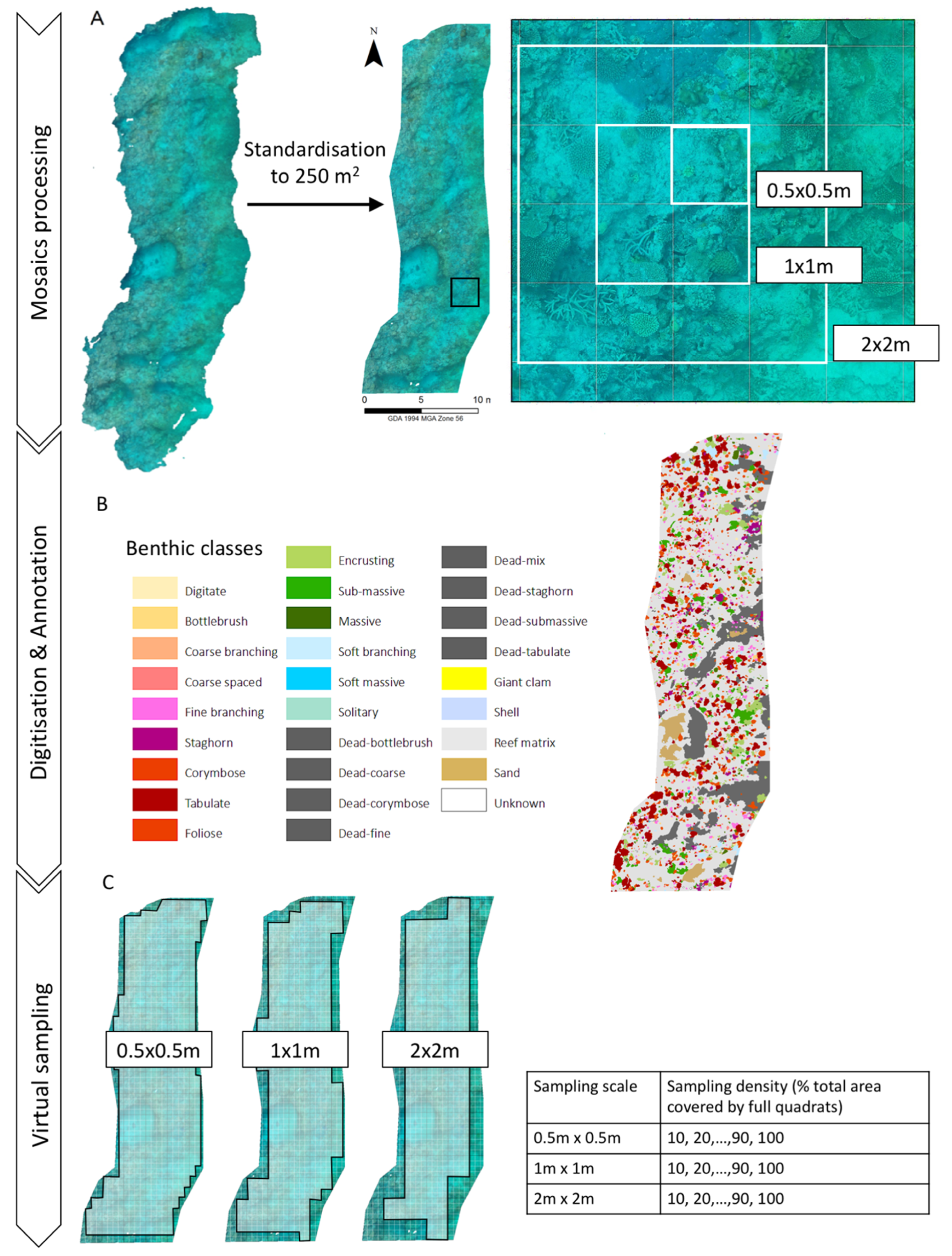
2.1. Study Site and Image Acquisition

Data were collected in January 2016, at eight reef slopes around Heron Reef (23.26′S, 151.54′E), Great Barrier Reef, Australia: Big Tub (BT), Harry’s Bommie (HB), Canyons (CA), Heron Bommie (HE), Pams Point (PP), Junction (JT), Blue Pools (BP), and Blue Pools East (BE) (Figure 1). Images were collected along one transect per site at depths of 5–10 m with transects following depth contours. Thirty-meter transects were mapped and modelled as per the methodology of Figueira et al. (2015) [15]. First, three visual references (30 cm-long uniquely coded targets) and two scale bars (50 cm PVC cylinders marked at 10 cm intervals) were deployed along each transect. These references are later used to scale the 3D models of the transects in the laboratory. Then three overlapping passes were done by SCUBA-divers with a custom mapping system flown 2–3m off the bottom. The mapping system consisted of three cameras (GoPro Hero4 Black, 12MP, Wide FOV, 4000 × 3000 pixels) equidistant apart (1 m), mounted on a 2 m long by 30 cm deep aluminium frames set to capture one image each per second. This protocol enabled a fast and non-destructive sampling of a 300 m² area of reef in approximately 7–10 min. This generated 1300–1800 images per transect from the three cameras, with an image footprint of approximately 5 × 4 m and 80% overlap in imagery [15]. Because only one transect was analysed per site, only the term ‘site’ will be used from this point. We aimed to identify optimal levels of sampling to characterise coral reef benthic communities within each site and not at reef level. As such, we intentionally selected sites that were very different and together represented the broad scale of heterogeneity found in shallow coral reef communities.

2.2. Model and Mosaics Generation

Images were imported and processed with the software package Photoscan Professional (v. 1.3) [24] which uses structure from motion algorithms to determine the relative position of all cameras from which a high-resolution photo mosaic of the whole area can be built. The high-resolution large-area mosaics [11] were created using a process adapted from Figueira [15] with the specific parameter values summarised in

Table 1. Description of parameter values and settings used in Photoscan (v.1.3., Agisoft, LLC) to build 3D models and 2D mosaics. Modified from Figueira et al. (2015).

Process	Settings	Comments
Photo alignment	High accuracy, pair selection enabled, key point limit 40000, tie point limit 4000, do not constrain features by mask	Align photos by common invariant key points resulting in a 3D sparse point cloud
Sparse point cloud	All optimisation properties yes except fit b1, b2; k4, p3, p4, rolling shutter	Optimisation of alignment based on camera and lenses properties
Dense point cloud	Medium quality, moderate depth filtering, do not reuse depth maps	Fill the sparse point cloud based on common points in the photos and camera locations
Mesh	Arbitrary surface type, source data-dense cloud face, count medium, interpolation enabled, all point classes	Create continuous 3D surface over dense cloud
Texture	Generic mapping mode, texture from all cameras, mosaic blending mode, texture size 8192, texture count 1, no color correction	Drape the original photos over the mesh
Mosaic building	Mesh surface type, mosaic blending mode, no color correction, hole filling enabled	Generate mosaic from mesh surface

. The resulting models were clipped to remove poorly resolved edges and scaled using the five scale features mentioned above. High resolution (0.911 ± 0.143 mm/pixel) 2D mosaics were then built and exported in TIFF format processing using geospatial software.

2.3. Digital Annotation of Benthic Organisms

All eight mosaics were standardised to a total area of 250 m² (25 × 10 m) (Figure 2A) except for one which was smaller (230 m²) due to defects around edges. Organisms were manually digitised by delineating them with polygons using editor tools in ArcGIS (ArcMap 10.3) [25]. Each polygon was stored in a shapefile or annotation layer, per site, and assigned to a specific subclass (Figure 2B). Cover area (m²) was automatically calculated for each polygon within ArcMap. The national Australian standard classification scheme Collaborative Annotation Tools for Analysis of Marine Imagery and Video (CATAMI) [26], with modifications to fit this study, was used to describe the benthos. ‘Reef matrix’ was used as an umbrella class to encompass organisms smaller than 10 cm, aggregates of dead organisms, rock, and rubble. Organisms smaller than 10 cm in diameter were excluded; ignoring small benthic organisms did not affect the overall result, because these were typically smaller versions of the same benthic class and thus overall diversity would not be greatly affected. This approach would not address specific questions with respect to small benthic organisms such as coral recruits. Only sessile organisms were accounted for. This procedure enabled the classification and the calculation of surface cover area for each benthic class. The total area annotation process of all organisms within one mosaic required 4–24 h to complete, depending on benthos heterogeneity and diversity.

2.4. Testing Different Sampling Efforts

To determine how many quadrats or how much area must be sampled to adequately estimate percent cover within each site, we first generated virtual quadrats and then resampled the dataset for each site across a range of sample densities. We tested three sampling quadrat sizes, 0.5 × 0.5 m, 1 × 1 m, and 2 × 2 m, representing a commonly used range of sampling scales [8,9,18,19,27,28]. Virtual quadrats were created from three grids (fishnets) of cell sizes corresponding to each quadrat size placed on top of each annotated mosaic (Figure 2C). Information about benthic organisms contained within each grid cell was then extracted by uniting the grids and the annotated mosaics (Analysis Toolbox > Union Tool). Datasets containing only full quadrats were loaded in R (v.3.3.3.) [29] and random virtual subsampling was undertaken with sample size set to the number of quadrats of each size required to sample 10, 20, 30, 40, 50, 60, 70, 80, 90, and 100% of the total area covered by the mesh (

Table 2. Correspondence between number of quadrats (NQuad) and total area sampled (m²) by each quadrat sizes for each site. Only quadrats that fitted completely on the mosaics were included in the analyses and thus, the total area sampled is lower for larger quadrat sizes as it was more likely they would include some non-mosaic components.

			Quadrat Size
	0.5 × 0.5 m		1 × 1 m		2 × 2 m
Sites	NQuad	Area	NQuad	Area	NQuad	Area
BE	928	232	206	206	43	172
BP	826	206.5	181	181	35	140
BT	914	228.5	205	205	41	164
CA	908	227	205	205	39	156
HB	922	230.5	204	204	42	168
HE	924	231	212	212	47	188
JT	912	228	208	208	42	168
PP	923	230.75	212	212	43	172

). For each mosaic and each quadrat size, this process was repeated 1000 times by selecting subsamples with replacement for each level of sample size. Subsampling with replacement was used as doing so without replacement creates a dependency amongst the datapoints (co-variance > 0) as the probability of selecting each becomes a function of the number of previously drawn points [30]. Relative standard error (RSE) amongst the 1000 samples was used to determine the precision of the cover area estimates for each class and each level of sample size. RSE was calculated as followed using $\overline{\mathrm{S}\mathrm{E}}$ and $\overline{\mathrm{X}}$, respectively standard error and mean cover of each benthic class

$$\mathrm{RSE}=\frac{\overline{\mathrm{SE}}}{\mathrm{X}¯}\times 100,$$

(1)

2.5. Data Analyses

2.5.1. Precision Level of Cover Estimates

For each combination of site, benthic class and quadrate size, the relationship between precision of cover estimates (relative standard error, RSE) and sample size (total area of site sampled) was evaluated to estimate the optimal sampling strategy. In all cases, this relationship followed a power function which approached an asymptotic RSE value (scaled by a) at a rate dictated by b

RSE = a(sample size)^b,

(2)

The a and b coefficients were estimated in Statistica (v.12.1, [31]) for each combination of quadrat size and benthic cover class using the non-linear estimation tool with a least squares loss function. In all cases, the power curves were fit with very high significance (p < 0.0001) and parameter estimates with very high precision (5% RSE at maximum and 0.62% on average). To evaluate the best sampling strategy, it is first necessary to define some criteria related to the acceptable level of RSE. Here, we used the approach of identifying a point on the diminishing returns curve where the improvement in RSE indicated that extra sampling was not warranted. This was done by assessing the value of sample size (on the x-axis) at which the slope (first derivative of y) of the power function exceeded a specific criterion (i.e., it got too shallow). The exact threshold value for this slope was determined by evaluating the first derivative curves of all relationships and choosing a slope threshold that was as close to zero as possible but which would intersect all curves within the 0–100% range (see Figure 3 for an example). In this case, the value −0.001 was chosen and this represents the target change in RSE per % area where further sampling would not result in valuable gain of precision. It is important to note that one could decide on a different value for this slope or even a different criterion altogether (sample effort required to achieve a specific RSE for instance). What is critical is that a common criterion is used against which to evaluate all sites, benthic classes, and quadrat size combinations.

Based on the methodology above, we calculated the proportion of the total area that needs to be sampled to hit the target change in RSE for every combination of site, benthic class, and quadrat size. We converted this into number of quadrats based on the size of the quadrat and the mosaic involved. These values, both represent the target sample size and are hereafter referred to as target-%Area and target-NQuad respectively.

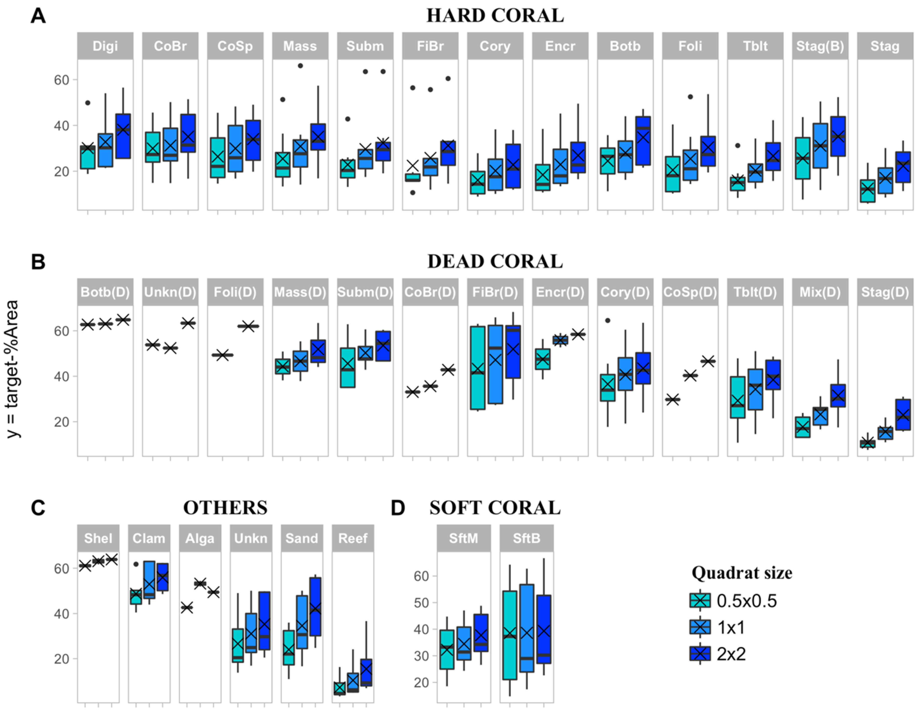
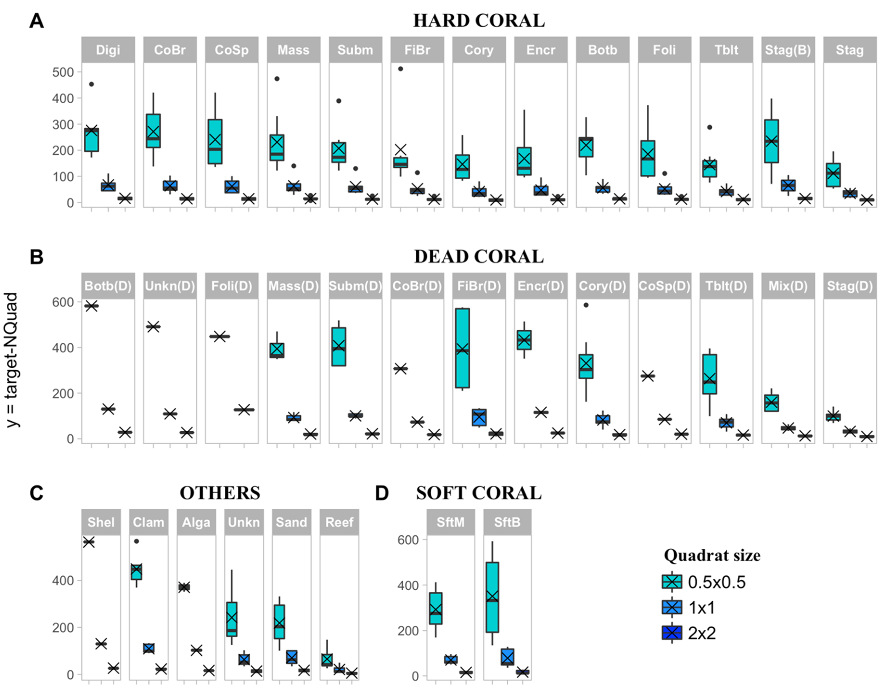
2.5.2. Effect of Quadrat Type, Benthic Class, and Cover on Target Sample Size

For all the following analyses, data were pooled across all sites. Three analyses were conducted to assess the factors that drive differences in percent area (target-%Area) and number of quadrats (target-NQuad). Even though the metric ‘number of quadrats’ seems redundant with area covered, and although it is expected that larger quadrats provide higher precision when number of quadrats is used as the metric for sampling effort [32], this has never been tested for coral reef monitoring programs and with in-situ data. Therefore, in this study, sampling effort is expressed in both percent area and number of quadrats. First, the effect of benthic class and quadrat size on the target-%Area was evaluated using a one-factor (quadrat size) ANOVA for each benthic class separately. This process was then repeated using target-NQuad as the response variable. Note, we did not attempt to include benthic class in a two-factor analysis given the very high number of levels and the extreme imbalance this would bring to the design. Only benthic classes which occurred in at least two of the eight sites for a given quadrat size were included. Assumptions of normality and homoscedasticity were assessed visually by plotting residuals and tested with Shapiro test and Levene’s test, respectively. Where a significant difference between quadrat size was found, Tukey’s HSD post-hoc test was run to determine which quadrat sizes were significantly different from each other.

Secondly, we tested the hypothesis that differences in target-%Area and target-NQuad may have more to do with the percent cover of a given benthic class rather than the identity of the benthic class itself. This was evaluated using a generalised linear model (in Statistica v12.1; [31]) with either target-%Area or target-NQuad as the response variable and two predictor variables, benthic class cover (continuous) and quadrat size (categorical, fixed, three-levels). Normality was checked visually, and homogeneity of variance assessed using Cochran’s test. Tukey’s HSD post-hoc test was used to determine which quadrat sizes were significantly different from each other.

Lastly, we investigated how the best sampling strategy proposed in this study affects how much of the taxonomic richness of an area would be captured reliably. This was evaluated by plotting the target sample size (area sampled for each quadrat size) against the proportion of benthic classes that would be adequately (according to the precision criteria given above) captured by following this strategy.

3. Results

Eight mosaics, with resolution of 0.911 ± 0.143 mm/pixel, were built, annotated within a standardised area of 250 m² and used to quantify cover estimates of benthic classes larger than 10 cm in diameter. The aim of this study was to identify optimal levels of sampling to characterise coral reef benthic communities within each site (and not at reef level). As such, the study sites were different and together represented the broad scale of heterogeneity found in shallow coral reef communities.

3.1. Percent Cover and Precision Target

A total of 42 benthic classes were identified and organised into eight coarse categories: abiotic, hard coral, soft coral, macroalgae, molluscs, dead coral, bleached coral, and unknown (

Table 3. Mean percent cover and codes for the key morphological classes of benthic features identified within the study area.

Coarse Categories	Benthic Classes	Codes	Mean Cover (%)	SE	Presence (No. of Sites)
Abiotic	Reef matrix	Reef	40.587	10.517	7
	Sand	Sand	3.038	1.442	7
Macroalgae	Algae	Alga	0.066	-	2
Hard corals	Bottlebrush	Btb	2.466	2.231	5
	Coarse branching	CoBr	0.151	0.042	7
	Coarse spaced	CoSp	0.418	0.120	8
	Columnar	Colu	0.039	0.029	2
	Corymbose	Cory	2.367	0.659	8
	Digitate	Figi	0.139	0.042	5
	Encrusting	Encr	2.654	0.734	8
	Fine branching	FiBr	1.618	0.889	6
	Foliose	Foli	4.372	1.713	8
	Foliose lettuce	FoLt	0.070	0/013	2
	Massive	Mass	0.899	0.260	8
	Solitary	Solt	0.012	0.001	5
	Staghorn	Stag	21.266	7.948	8
	Submassive	Subm	1.035	0.384	7
	Tabulate	Tblt	5.362	2.027	8
Soft corals	Soft branching	SftB	0.444	0.185	8
	Soft massive	SftM	0.274	0.136	7
Bleached corals	Bottlebrush	Btb(B)	0.031	-	1
	Coarse branching	CoBr(B)	0.003	-	1
	Corymbose	Cory(B)	0.031	0.009	2
	Fine branching	FiBr(B)	0.010	-	1
	Staghorn	Stag(B)	17.322	17.131	2
	Soft massive	SftM(B)	0.014	-	1
Dead corals	Bottlebrush	Btb(D)	0.004	-	1
	Coarse branching	CoBr(D)	0.039	-	1
	Coarse spaced	CoSp(D)	0.561	-	1
	Corymbose	Cory(D)	0.213	0.089	7
	Encrusting	Encr(D)	0.185	0.096	2
	Fine branching	FiBr(D)	0.088	0.043	5
	Foliose	Foli(D)	0.039	-	1
	Massive	Mass(D)	0.030	0.014	3
	Mix	Mix(D)	3.033	1.001	7
	Staghorn	Stag(D)	15.530	4.2	5
	Submassive	Subm(D)	0.093	0.037	5
	Tabulate	Tblt(D)	2.023	1.571	8
	Unknown	Unkn(D)	0.006	-	1
Molluscs	Giant clam	Clam	0.011	0.003	6
	Shell	Shel	0.001	1.28E-05	2
Unknown	Unknown	Unkn	0.799	0.292	7

). The coarse category ‘abiotic’ describes sandy areas, the rocky matrix and cement platforms or eroded surfaces that cannot be distinguished as dead organisms. The term ‘macroalgae’ encompasses algae patches larger than 10 cm in diameter and does not include turf algae. ‘Dead coral’ represents coral that recently died and are still morphologically identifiable with higher complexity than the rocky matrix. Four out of 42 benthic classes; reef matrix, staghorn, bleached staghorn, and dead staghorn; had the highest mean percent covers from 40.6% to 15.5%. Ten benthic classes showed medium to low mean percent cover from 5.4% to 1%, and 28 were low (<1%) (Table 3).

3.2. Effect of Sampling Strategy and Benthic Class on Target Sample Size

When sample size was expressed as percent area, there was a trend for the smallest quadrat size to correspond to the smallest sampling size required for all benthic classes. However, variability in percent cover was high and this was only significant for the benthic classes staghorn, tabulate, dead mix, and dead staghorn (

Table A1. Summary of one-way ANOVA investigating the effect of quadrat size on sample size (% Area) for each benthic class with at least two observations per quadrat size. Significant differences (p < 0.05) are in bold.

Target Sample size		Percent Area						No. of Quadrats
		Df	Sum Sq	Mean Sq	F	p		Df	Sum Sq	Mean Sq	F	p
Botb	Quadrat size	2	275.22	137.61	1.1544	0.3479		2	117674	58837	23.361	7.28E-05
	Residuals	12	1430.45	1.565	119.2			12	30224	2519
Clam	Quadrat size	2	146.07	73.034	1.2123	0.329		2	564160	282080	146.11	1.23E-09
	Residuals	13	783.15	60.242				13	25098	1931
CoBr	Quadrat size	2	102.27	51.135	0.3399	0.7163		2	260553	130277	32.592	1.04E-06
	Residuals	18	2708.13	150.452				18	71950	3997
Cory	Quadrat size	2	186.7	93.352	1.048	0.3683		2	82133	41066	25.044	2.75E-06
	Residuals	21	1870.6	89.075				21	34436	1640
CoSp	Quadrat size	2	233.68	116.84	0.8117	0.4576		2	228353	114177	26.698	1.71E-06
	Residuals	21	3022.86	143.95				21	89809	4277
Digi	Quadrat size	2	166.88	83.438	0.4972	0.6203		2	189489	94744	22.005	9.67E-05
	Residuals	12	2013.99	167.832				12	51667	4306
Encr	Quadrat size	2	287.71	143.85	1.285	0.2975		2	107546	53773	18.836	2.06E-05
	Residuals	21	2350.89	111.95				21	59950	2855
FiBr	Quadrat size	2	238.5	119.25	0.4608	0.6394		2	119947	59974	7.2632	0.006225
	Residuals	15	3881.6	258.77				15	123858	8257
Foli	Quadrat size	2	397.02	198.51	1.3882	0.2715		2	131277	65639	18.451	2.37E-05
	Residuals	21	3002.9	143				21	74707	3557
FoLt	Quadrat size	2	6.88	3.44	0.1784	0.8449		2	218961	109481	7914.3	2.61E-06
	Residuals	3	57.855	19.285				3	41	14
Mass	Quadrat size	2	374.7	187.33	0.9875	0.3892		2	206114	103057	20.685	1.09E-05
	Residuals	21	3983.9	189.71				21	104628	4982
SftB	Quadrat size	2	2.5	1.24	0.0032	0.9968		2	461072	230536	15.881	0.000106
	Residuals	18	6933.1	385.17				18	261301	14517
SftM	Quadrat size	2	104.96	52.478	0.6492	0.5343		2	300646	150323	52.69	2.99E-08
	Residuals	18	1454.96	80.831				18	51353	2853
Solt	Quadrat size	2	341.54	170.77	2.4406	0.129		2	374506	187253	354.27	2.13E-11
	Residuals	12	839.64	69.97				12	6343	529
Stag	Quadrat size	2	391.59	195.796	3.5357	0.04748		2	45476	22738	22.9	5.29E-06
	Residuals	21	1162.91	55.377				21	20851	992.9
Subm	Quadrat size	2	333.6	166.79	0.8934	0.4266		2	143260	71630	23.342	1.00E-05
	Residuals	18	3360.4	186.69				18	55237	3069
Tblt	Quadrat size	2	469.28	234.638	3.8217	0.03842		2	78552	39276	24.79	2.97E-06
	Residuals	21	1289.3	61.395				21	33272	1584
Unkn	Quadrat size	2	263.21	131.6	0.7905	0.4688		2	201303	100651	20.658	2.18E-05
	Residuals	18	2996.82	166.49				18	87701	4872
Cory(B)	Quadrat size	2	27.49	13.745	0.5348	0.6329		2	195406	97703	130.47	0.001212
	Residuals	3	77.11	25.703				3	2246	749
Stag(B)	Quadrat size	2	91.9	45.95	0.0695	0.9344		2	52940	26470	1.399	0.3722
	Residuals	3	1984.9	661.64				3	56762	18921
Cory(D)	Quadrat size	2	168.6	84.303	0.4365	0.6529		2	382833	191416	29.018	2.34E-06
	Residuals	18	3476.3	193.127				18	118735	6596
FiBr(D)	Quadrat size	2	187.3	93.63	0.2898	0.7535		2	387327	193663	17.416	0.0002831
	Residuals	12	3876.6	323.05				12	133441	11120
Mass(D)	Quadrat size	2	89.63	44.813	0.607	0.5754		2	235661	117830	73.313	6.08E-05
	Residuals	6	442.99	73.832				6	9643	1607
Mix(D)	Quadrat size	2	676.97	338.49	6.961	0.005763		2	83397	41698	66.709	4.74E-09
	Residuals	18	875.27	48.63				18	11251	625
Stag(D)	Quadrat size	2	374.79	187.395	7.0763	0.009332		2	21892.8	10946.4	38.776	5.79E-06
	Residuals	12	317.78	26.482				12	3387.6	282.3
Subm(D)	Quadrat size	2	159.11	79.553	1.0112	0.3928		2	416424	208212	72.214	2.04E-07
	Residuals	12	944.05	78.671				12	34599	2883
Tblt(D)	Quadrat size	2	339.76	169.88	1.2176	0.316		2	271546	135773	33.733	2.77E-07
	Residuals	21	2929.86	139.52				21	84523	4025

, Figure 4). Tukey’s HSD post hoc test revealed that 2 × 2 m quadrats were always significantly different from 0.5 × 0.5 m for staghorn (p = 0.038), tabulate (p = 0.031), dead mix (p = 0.004) and dead staghorn (p = 0.007); but none was different from 1 × 1 m for those classes (p > 0.05).

When sample size was expressed as number of quadrats, there was a significant effect of quadrat size for all benthic classes except bleached staghorn (Table A1, Figure 5). The number of quadrats decreased when quadrat sizes increased for all classes, though Tukey’s HSD post hoc test revealed the differences were only significant between quadrat size 0.5 × 0.5 m and 1 × 1 m and between 0.5 × 0.5 m and 2 × 2 m. There was no difference between 1 × 1 m and 2 × 2 m for all benthic classes.

Apparent patterns are highlighted in Figure 5 which shows differences in target sampling effort between the different classes. Although differences were not statistically evaluated, there were clear patterns where certain classes had a low target effort while it was higher for others. For instance, reaching the target precision required a low sampling effort (<10% Area) for reef matrix (Reef), staghorn (Stag) and dead staghorn (Stag(D)) Figure 5A–C), regardless of quadrat size. Intermediate sampling effort (20–50% Area) was required for most classes and high sampling effort (>50% Area) was required to capture shell (Shel), algae (Alga), and dead bottlebrush (Botb(D)) (Figure 5B,C).

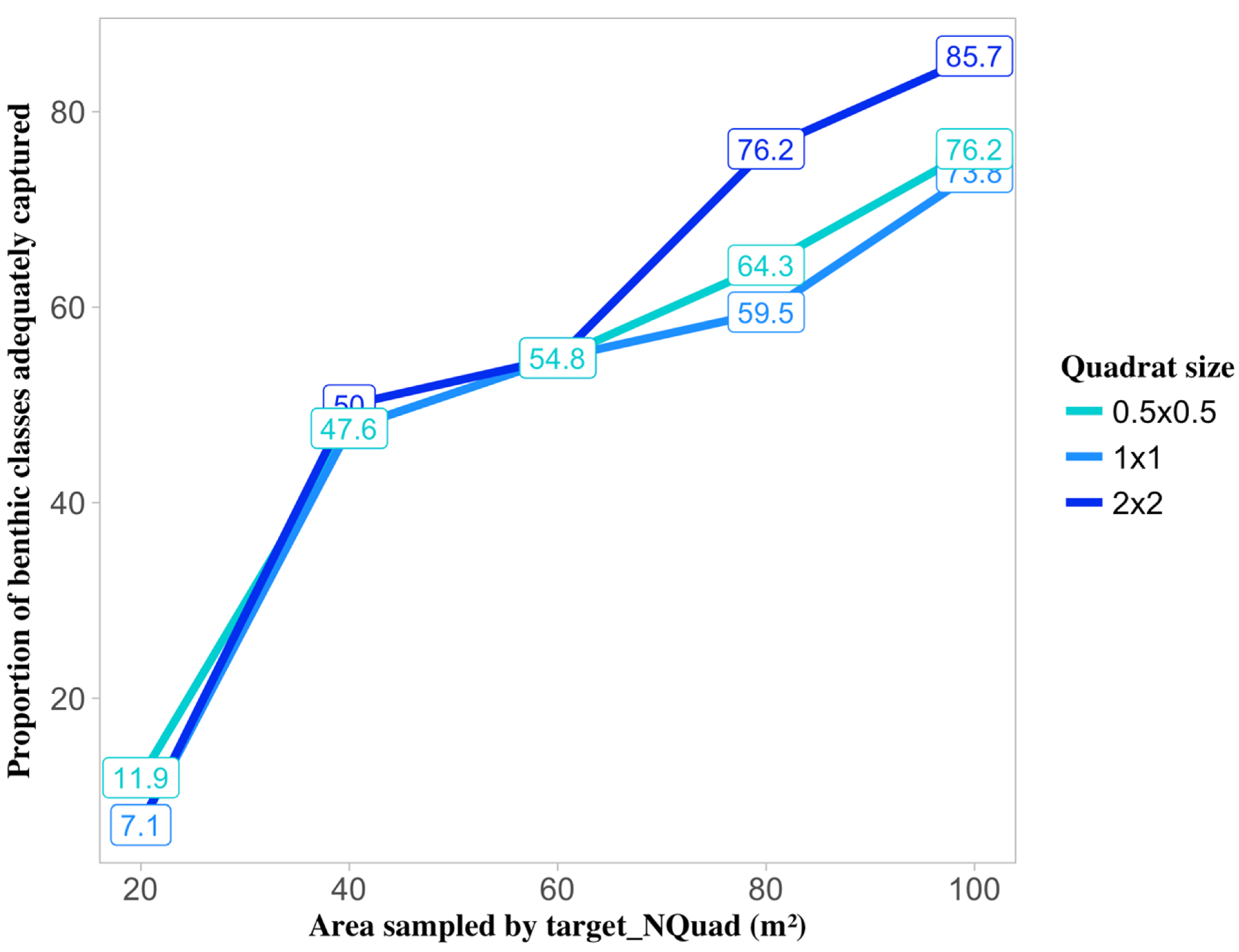
3.3. Effect of Sampling Strategy and Cover on Target Sample Size

Overall, percent cover had a greater effect on sampling density than the identity of the benthic class itself. Indeed, low cover classes (i.e., rare, <1% mean cover) required a rather high level of sampling, from 40% up to 65% of the total area sampled, to be adequately represented. In contrast, organisms that had high coverage across the study area (i.e., 15–40% mean cover) only required a level of sampling ≤30% of the total area to be adequately captured (Figure 5 and Figure 6). Such conspicuous organisms would act as good candidates for long-term monitoring as the sampling effort required to gain accurate and precise estimates of their coverage would be more efficient. These findings were supported when the percent cover of all organisms was plotted against sampling density (Figure 6).

Significant differences in sampling size for both metrics were found between quadrat sizes. The effect of quadrat size was significant considering either number of quadrats (F₂₅₆₇ = 1298.2, p < 0.001) or percent area (F₂₂₆₇ = 63.8, p < 0.001) as was the effect of percent cover (F_NQuad(1567) = 1402.8, p_NQuad < 0.001; F_%Area(2567) = 2044.3, p_%Area < 0.001). The interaction of these factors was significant when sample size was expressed as number of quadrats (F₂₅₆₇ = 691.9, p < 0.001) but not for the percent area. Post-hoc Tukey’s HSD tests revealed that in both cases, all quadrat sizes were significantly different from each other (p < 0.0001). However, a visual comparison of sample size means shows that, when using percent area, the difference between quadrat sizes was subtle (mean response varies by about 10%) and uniform over percent cover. When using the number of quadrats as the measure of sampling effort however, the effects of quadrat size were more clear-cut (mean responses varied by up to 45%) and were strongly dependent on the percent cover of the benthic class identified, this was most pronounced for the less abundant classes.

These findings suggest that it is possible to determine how much area should be sampled with minimal information about abundance, prior to the survey campaign. For instance, to adequately (meet the target precision) sample 55% of all benthic classes present at the study site, the area sampled needs to be equivalent to 60 m², corresponding to 240 0.5 × 0.5 m quadrats (240 × 0.25 m²), 60 1 × 1 m quadrats (60 × 1 m²) and 15 2 × 2m quadrats (15 × 4 m²) (Figure 7).

4. Discussion

We used high-resolution large-area mosaics to assess the accuracy and precision of traditional photo-based benthic sampling methods in coral reefs. This study did not intent to characterise the benthos at reef level. The aim of this study was to identify the optimal level of sampling (highest target precision for the least effort) to characterise coral reef benthic communities (whatever they are) within each site. The study sites were intentionally selected to be different and together represented the broad scale of heterogeneity found in shallow coral reef communities. The results revealed no significant difference in sample size whether the metric used was percent area or number of quadrats, but there was a significant difference between quadrat size. The 2 × 2 m quadrat size was the most efficient (or optimal according to this study) because it corresponded to the least effort (number of quadrats or area sampled, see Figure 7)). Overall, the most abundant benthic classes required the lowest sampling effort to deliver reliable (high precision) cover estimates. These results suggest that sampling effort is related to percent cover and thus provide an estimate of the level of sampling required to capture specific proportions. Existing data on abundance can be used in combination with the relationships presented here as a basis for determining the optimal sampling protocols for ongoing coral reef monitoring. Because this study aimed at generating relevant advice to practitioners, we chose to subsample from the maximum area covered by full quadrats. It is important to mention that while it might have been better to subsample smaller quadrats from within the larger quadrat size this would have not reflected real world monitoring. It is however important to keep in mind this while interpreting the results, in short, we wanted to address our research question from a sampling perspective and find what is optimal for each quadrat size.

The choice of sampling strategy for photoquadrat-based methods has been assessed in previous studies. These studies suggest that large quadrat sizes are more efficient [9] and when field time is limited, larger quadrat sizes should be used [33]. Importantly, we found the use of larger quadrat size appropriate when sampling effort is expressed as number of quadrats. In this case, more area can be covered by using larger quadrats. However, larger quadrats can come at the cost of data resolution. For example, fewer points per area in the case of in-situ point counts (if the number of points is conserved throughout quadrat sizes then resolution is lessened) or lower image resolution for photoquadrats (as the picture will be taken from a distance). In situations where it is desired to maintain resolution, sampling effort will scale with percent area rather than number of quadrats (e.g., need to take more photos at larger ‘quadrat’ sizes). In this situation, our work suggests smaller quadrat sizes are in fact more efficient (higher resolution) because they correspond to the highest precision. Ultimately, the choice of sampling strategy will depend on the spatial distribution of the target biota and how overall effort is tied to number of replicates versus total area. Therefore, the key factor will be the relative cost of field time versus annotation/scoring time. For in-situ photo-based sampling, field costs can be minimised by sampling fewer larger quadrats, but this will result in lower resolution photos to cover the larger area. To increase image resolution, multiple photos are needed to cover the larger area and thus time-cost in field is not reduced. Analysis cost could also be minimised with fewer larger quadrats but only if another cover estimation method than total area annotation is used, for example using point counts with low point densities per quadrat. However, using less quadrats or low point densities per quadrat will result in lower precision of estimates. One affordable and time-saving solution would be to use more than one camera at a time as in this study. Another solution would be to target taxa groups with dominant coverage in the system that can be monitored at lower resolution [18].

To date, the main limitations of traditional sampling approaches consist in the fact that they have been restricted to relatively small spatial scales because of the high-cost associated with getting high-resolution data over large areas [6,34]; or they used remote sensing techniques resulting in coarser spatial resolution data provision [35]. The application of close-range photogrammetry based on SfM algorithms presented here, along with techniques recently developed (e.g., autonomous and semi-autonomous underwater vehicles), can help fill the need for wider areal coverage (kilometre scales) and high spatial resolution (meter to sub-centimetre scale) data provision [5,11,12,36] to ensure current and comprehensive benthic composition mapping [37]. Moreover, to overcome the sampling limitation of assessing the true value of the parameter being quantified for a given area, high-resolution large-area imaging allows the acquisition of data (high-resolution digitisation of cover) that can be used as a baseline or ‘truth’ against which cover estimates would be compared [20].

In the future, repeated measurements of the same sites can be done to assess whether the sampling strategies presented here are able to detect changes in coral cover over time. More interesting investigations involving the use of this method would be to take random sample of the reef studied and assess the interaction between the number of quadrats required and the number of sites required to sample different patches of the reef. The use of large-area mosaics proved to be a promising tool for accessing high-resolution percentage cover estimates over a range of spatial and temporal scales and it is compatible with existing photoquadrat methods. This can then serve as the basis for developing new or alternate sampling designs and would allow a gradual transition from one to the other for coral reef monitoring. For instance, the approach presented here could be applicable to optimise point count as it is also quadrat-based sampling, only percent area is estimated from point intercept rather than tracing. The likely outcome of this would be increased target sample sizes (more quadrats needed to hit target) because the variance between subsamples will be greater due to the extra variance from another level of sampling within the quadrats (random placement of points). This study provides novelty in examining how differences sampling strategies influence the accuracy and precision of percent cover estimates derived from in-situ data (i.e. not simulated). Given the decline projections for coral reef trajectories, future sample points are more likely to present homogeneous communities and lower percent cover and thus, the guidelines set in this study and the importance to define adequate precision level will still be coherent to represent future communities as the work presented here specifically highlighted the effect of cover of taxa.

5. Conclusions

The use of underwater imagery as a tool for benthic monitoring is widespread. Here we provide guidance to scientists and managers conducting such surveys in quadrat-based sampling strategies that would deliver accurate and precise cover estimates. Results show that each of the benthic classes has different optimal sampling sizes to be adequately sampled within a given framework. For example, a sampling size equivalent to 60 m² of the total area sampled by all quadrats is needed to provide representative cover estimates of 55% of all benthic features at the target precision. Pilot study data on abundance can be used in combination with the relationships presented here as a basis to determine the optimal sampling protocols for ongoing coral reef monitoring.

References

1. Pandolfi, J.M.; Bradbury, R.H.; Sala, E.; Hughes, T.P.; Bjorndal, K.A.; Cooke, R.G.; McArdle, D.; McClenachan, L.; Newman, M.J.H.; Paredes, G. Global trajectories of the long-term decline of coral reef ecosystems. Science 2003, 301, 955–958. [Google Scholar] [CrossRef] [Green Version]
2. Hughes, T.P.; Kerry, J.T.; Alvarez-Noriega, M.; Alvarez-Romero, J.G.; Anderson, K.D.; Baird, A.H.; Babcock, R.C.; Beger, M.; Bellwood, D.R.; Berkelmans, R.; et al. Global warming and recurrent mass bleaching of corals. Nature 2017, 543, 373–377. [Google Scholar] [CrossRef] [PubMed]
3. De’ath, G.; Fabricius, K.E.; Sweatman, H.; Puotinen, M. The 27-year decline of coral cover on the Great Barrier Reef and its causes. Proc. Natl. Acad. Sci. USA 2012, 109, 17995–17999. [Google Scholar] [CrossRef] [PubMed] [Green Version]
4. Hughes, T.P.; Rodrigues, M.J.; Bellwood, D.R.; Ceccarelli, D.; Hoegh-Guldberg, O.; McCook, L.; Moltschaniwskyj, N.; Pratchett, M.S.; Steneck, R.S.; Willis, B.L. Phase shifts, herbivory, and the resilience of coral reefs to climate change. Curr. Biol. 2007, 17, 360–365. [Google Scholar] [CrossRef] [PubMed] [Green Version]
5. Ferrari, R.; Bryson, M.; Bridge, T.; Hustache, J.; Williams, S.B.; Byrne, M.; Figueira, W. Quantifying the response of structural complexity and community composition to environmental change in marine communities. Glob. Chang. Biol. 2016, 22, 1965–1975. [Google Scholar] [CrossRef] [PubMed]
6. Hedley, J.D.; Roelfsema, C.M.; Chollett, I.; Harborne, A.R.; Heron, S.F.; Weeks, S.; Skirving, W.J.; Strong, A.E.; Eakin, C.M.; Christensen, T.R. Remote sensing of coral reefs for monitoring and management: A review. Remote Sens. 2016, 8, 118. [Google Scholar] [CrossRef] [Green Version]
7. Boström, C.; Pittman, S.J.; Simenstad, C.; Kneib, R.T. Seascape ecology of coastal biogenic habitats: Advances, gaps, and challenges. Mar. Ecol. Prog. Ser. 2011, 427, 191–217. [Google Scholar] [CrossRef] [Green Version]
8. Jonker, M.M.; Johns, K.K.; Osborne, K.K. Surveys of benthic reef communities using underwater digital photography and counts of juvenile corals. In Long--term Monitoring of the Great Barrier Reef. Standard Operational Procedure. 2008. Available online: https://www.aims.gov.au/docs/research/monitoring/reef/sops.html (accessed on 13 November 2019).
9. Palma, M.; Rivas Casado, M.; Pantaleo, U.; Cerrano, C. High Resolution Orthomosaics of African Coral Reefs: A Tool for Wide-Scale Benthic Monitoring. Remote Sens. 2017, 9, 705. [Google Scholar] [CrossRef] [Green Version]
10. Pizarro, O.; Friedman, A.; Bryson, M.; Williams, S.B.; Madin, J. A simple, fast, and repeatable survey method for underwater visual 3D benthic mapping and monitoring. Ecol. Evol. 2017, 7, 1770–1782. [Google Scholar] [CrossRef]
11. Edwards, C.B.; Eynaud, Y.; Williams, G.J.; Pedersen, N.E.; Zgliczynski, B.J.; Gleason, A.C.; Smith, J.E.; Sandin, S.A. Large-area imaging reveals biologically driven non-random spatial patterns of corals at a remote reef. Coral Reefs 2017, 36, 1291–1305. [Google Scholar] [CrossRef] [Green Version]
12. González-Rivero, M.; Beijbom, O.; Rodriguez-Ramirez, A.; Holtrop, T.; González-Marrero, Y.; Ganase, A.; Roelfsema, C.; Phinn, S.; Hoegh-Guldberg, O. Scaling up ecological measurements of coral reefs using semi-automated field image collection and analysis. Remote Sens. 2016, 8, 30. [Google Scholar] [CrossRef] [Green Version]
13. Bryson, M.; Ferrari, R.; Figueira, W.; Pizarro, O.; Madin, J.; Williams, S.B.; Byrne, M. Characterization of measurement errors using structure-from-motion and photogrammetry to measure marine habitat structural complexity. Ecol. Evol. 2017, 7, 5669–5681. [Google Scholar] [CrossRef] [PubMed]
14. Burns, J.H.R.; Delparte, D.; Kapono, L.; Belt, M.; Gates, R.D.; Takabayashi, M. Assessing the impact of acute disturbances on the structure and composition of a coral community using innovative 3D reconstruction techniques. Methods Oceanogr. 2016, 15–16, 49–59. [Google Scholar] [CrossRef] [Green Version]
15. Figueira, W.; Ferrari, R.; Weatherby, E.; Porter, A.; Hawes, S.; Byrne, M. Accuracy and Precision of Habitat Structural Complexity Metrics Derived from Underwater Photogrammetry. Remote Sens. 2015, 7, 16883–16900. [Google Scholar] [CrossRef] [Green Version]
16. Beijbom, O.; Edmunds, P.J.; Roelfsema, C.; Smith, J.; Kline, D.I.; Neal, B.P.; Dunlap, M.J.; Moriarty, V.; Fan, T.-Y.; Tan, C.-J. Towards automated annotation of benthic survey images: Variability of human experts and operational modes of automation. PLoS ONE 2015, 10, e0130312. [Google Scholar] [CrossRef] [PubMed]
17. Leujak, W.; Ormond, R.F.G. Comparative accuracy and efficiency of six coral community survey methods. J. Exp. Mar. Biol. Ecol. 2007, 351, 168–187. [Google Scholar] [CrossRef]
18. Perkins, N.R.; Foster, S.D.; Hill, N.A.; Barrett, N.S. Image subsampling and point scoring approaches for large-scale marine benthic monitoring programs. Estuar. Coast. Shelf Sci. 2016, 176, 36–46. [Google Scholar] [CrossRef]
19. Brown, E.K.; Cox, E.; Jokiel, P.; Rodgers, S.K.u.; Smith, W.R.; Tissot, B.N.; Coles, S.L.; Hultquist, J. Development of benthic sampling methods for the Coral Reef Assessment and Monitoring Program (CRAMP) in Hawai’i. Pac. Sci. 2004, 58, 145–158. [Google Scholar] [CrossRef] [Green Version]
20. Mapstone, B.D.; Ayling, T. An Investigation of Optimum Methods and Unit Sizes for the Visual Estimation of Abundances of Some Coral Reef Organisms (No. 47); Great Barrier Reef Marine Park Authority: Townsville, Australia, 1998.
21. Brown, C.J.; Smith, S.J.; Lawton, P.; Anderson, J.T. Benthic habitat mapping: A review of progress towards improved understanding of the spatial ecology of the seafloor using acoustic techniques. Estuar. Coast. Shelf Sci. 2011, 92, 502–520. [Google Scholar] [CrossRef]
22. Lecours, V.; Devillers, R.; Schneider, D.C.; Lucieer, V.L.; Brown, C.J.; Edinger, E.N. Spatial scale and geographic context in benthic habitat mapping: Review and future directions. Mar. Ecol. Prog. Ser. 2015, 535, 259–284. [Google Scholar] [CrossRef] [Green Version]
23. GBRMPA. Great Barrier Reef Marine Park Authority Spatial Data Geoportal. Available online: http://www.gbrmpa.gov.au/geoportal/catalog/download/download.page (accessed on 31 May 2017).
24. Agisoft LLC. Agisoft Photoscan User Manual; Professional Edition v. 1. 3; Agisoft LLC: St Petersburg, Russia, 2014. [Google Scholar]
25. ESRI Inc. ArcGIS 10.3; ESRI Inc.: Redlands, CA, USA, 2004. [Google Scholar]
26. Althaus, F.; Hill, N.; Ferrari, R.; Edwards, L.; Przeslawski, R.; Schönberg, C.H.; Stuart-Smith, R.; Barrett, N.; Edgar, G.; Colquhoun, J. A standardised vocabulary for identifying benthic biota and substrata from underwater imagery: The CATAMI classification scheme. PLoS ONE 2015, 10, e0141039. [Google Scholar] [CrossRef]
27. Jokiel, P.L.; Rodgers, K.S.; Brown, E.K.; Kenyon, J.C.; Aeby, G.; Smith, W.R.; Farrell, F. Comparison of methods used to estimate coral cover in the Hawaiian Islands. PeerJ 2015, 3, e954. [Google Scholar] [CrossRef] [PubMed] [Green Version]
28. Roberts, T.; Moloney, J.; Sweatman, H.; Bridge, T. Benthic community composition on submerged reefs in the central Great Barrier Reef. Coral Reefs 2015, 34, 569–580. [Google Scholar] [CrossRef]
29. R Core Team. The R Project for Statistical Computing. Available online: http://www.R-project.org/ (accessed on 31 May 2017).
30. Kendall, W.L.; White, G.C. A cautionary note on substituting spatial subunits for repeated temporal sampling in studies of site occupancy. J. Appl. Ecol. 2009, 46, 1182–1188. [Google Scholar] [CrossRef]
31. TIBCO Software Inc. Statistica v. 12.1; TIBCO Software Inc.: Palo Alto, CA, USA, 2017. [Google Scholar]
32. Kowalewski, L.K.; Chizinski, C.J.; Powell, L.A.; Pope, K.L.; Pegg, M.A. Accuracy or precision: Implications of sample design and methodology on abundance estimation. Ecol. Model. 2015, 316, 185–190. [Google Scholar] [CrossRef] [Green Version]
33. Pringle, J. Efficiency estimates for various quadrat sizes used in benthic sampling. Can. J. Fish. Aquat. Sci. 1984, 41, 1485–1489. [Google Scholar] [CrossRef]
34. Roelfsema, C.; Phinn, S.; Udy, N.; Maxwell, P. An integrated field and remote sensing approach for mapping seagrass cover, Moreton Bay, Australia. J. Spat. Sci. 2009, 54, 45–62. [Google Scholar] [CrossRef]
35. Hedley, J.D.; Roelfsema, C.M.; Phinn, S.R.; Mumby, P.J. Environmental and sensor limitations in optical remote sensing of coral reefs: Implications for monitoring and sensor design. Remote Sens. 2012, 4, 271–302. [Google Scholar] [CrossRef] [Green Version]
36. Ferrari, R.; Malcolm, H.; Neilson, J.; Lucieer, V.; Jordan, A.; Ingleton, T.; Figueira, W.; Johnstone, N.; Hill, N. Integrating distribution models and habitat classification maps into marine protected area planning. Estuar. Coast. Shelf Sci. 2018, 212, 40–50. [Google Scholar] [CrossRef] [Green Version]
37. Roelfsema, C.; Kovacs, E.; Ortiz, J.C.; Wolff, N.H.; Callaghan, D.; Wettle, M.; Ronan, M.; Hamylton, S.M.; Mumby, P.J.; Phinn, S. Coral reef habitat mapping: A combination of object-based image analysis and ecological modelling. Remote Sens. Environ. 2018, 208, 27–41. [Google Scholar] [CrossRef]
Figure 1. Study site. Heron Reef is located within the Capricorn Bunker Group in the Southern GBR. The eight sites are represented by their codes: Big Tub (BT), Harry’s Bommie (HB), Canyons (CA), Heron Bommie (HE), Pams Point (PP), Junction (JT), Blue Pools (BP), and Blue Pools East (BE). Image sources: GBR and Capricorn Bunker Group—GBRMPA Geoportal [23]; Heron Reef satellite image— Heron Island, Queensland, 23°28′35.16”S, 151°51′43.27”E, eye alt 16.83 km, Landsat/Copernicus, Maxar Technologies 2019, Google Earth Pro v. 7.3.2.5776 (4 July 2016).
Remotesensing 11 02907 g001
Figure 2. Schematic workflow overview for mosaic processing and analyses: (A) processed and standardised mosaic of a site (left) and the detail of the sampling scales applied (right); (B) digitised output showing the cover of different benthic classes; (C) total area covered by all quadrat of each size (left) and summary of sampling scales and quadrat densities tested (right).
Remotesensing 11 02907 g002
Figure 3. Example of how the precision level (target change in RSE per unit percent area) was identified. The relative standard error (RSE) (A) and the slope (first derivative) of RSE (B) were plotted against the total % area sampled for ten different curves (cover types) to represent the full range (mean cover 0.003–40.6%) observed in the dataset (the thickest line represents the most abundant type and the finest the least abundant). The red line in (B) shows the threshold value for slope used in this study. The corresponding value on each curve in (A) is indicated by a red dot.
Remotesensing 11 02907 g003
Figure 4. Differences in target sample size, expressed as target-%Area, between quadrat sizes and benthic classes. Benthic classes are grouped as follow: (A) Hard coral, (B) dead coral, (C) others, and (D) soft coral. Benthic organisms with little variation are omitted, hence the difference in grouping. Within plot with n(classes)>2, classes are arranged by mean total percent cover, from lowest on the left to highest on the right. The boxplots show the first, second (median) and third quartiles. The upper whisker extends from the hinge to the largest value no further than 1.5 × IQR from the hinge (where IQR is the inter-quartile range, or distance between the first and third quartiles). The lower whisker extends from the hinge to the smallest value at most 1.5 × IQR of the hinge. Circles and crosses represent outliers and means, respectively.
Remotesensing 11 02907 g004
Figure 5. Differences in target sample size, expressed as target-NQuad, between quadrat sizes and benthic classes. Benthic classes are grouped as follow: (A) Hard coral, (B) dead coral, (C) others, and (D) soft coral. Benthic organisms with little variation are omitted, hence the difference in grouping. Within plot with n(classes)>2, classes are arranged by mean total percent cover, from lowest on the left to highest on the right. The boxplots show the first, second (median) and third quartiles. The upper whisker extends from the hinge to the largest value no further than 1.5 × IQR from the hinge (where IQR is the inter-quartile range, or distance between the first and third quartiles). The lower whisker extends from the hinge to the smallest value at most 1.5 × IQR of the hinge. Circles and crosses represent outliers and means, respectively.
Remotesensing 11 02907 g005
Figure 6. Relationship between percent cover and target sample size. Covers are displayed on a log-axis against target sample size expressed as either target-%Area (A) or target-NQuad (B).
Remotesensing 11 02907 g006
Figure 7. Proportion of benthic classes adequately (with the given level of precision set for this study) captured regarding the area covered by quadrats for each quadrat size: 0.5 × 0.5 m, 1 × 1 m, and 2 × 2 m.
Remotesensing 11 02907 g007