1. Introduction
The production of accurate land use/land cover (LULC) maps offers unique monitoring capabilities within the remote sensing domain [
1]. LULC maps are being used for a variety of applications, ranging from environmental monitoring, land change detection, and natural hazard assessment to agriculture and water/wetland monitoring [
2]; therefore, accurate and timely production of LULC maps is of great significance. LULC maps are usually produced by two main procedures: photo-interpretation by the human eye, which is time and resource consuming and is not suitable for operational LULC-mapping over large areas; and second, automatic mapping using remotely sensed data and different classification algorithms.
The availability and a swift update of high-quality satellite remote sensing data has brought tremendous progress in providing up-to-date and accurate land cover information. Multispectral images, particularly, are an essential resource for building LULC maps, allowing for the use of classification algorithms to automate their production. Although significant progress has been made in the use of supervised learning techniques for automatic image classification [
3], the acquisition of labeled training sets continues to be a bottleneck [
4]. In order to build accurate and robust supervised classifiers it is crucial to have a large enough training dataset. Often, the problem is that different land cover types have very different levels of area coverage, which causes some of them to be frequent in the training dataset, while others are limited [
5].
A particular case where this phenomenon happens is the LUCAS dataset: Land Use and Coverage Area frame Survey coordinated by The Statistical Office of the European Commission (Eurostat) [
6]. LUCAS surveys have been carried out every three-years since 2006 and are freely accessible. For this statistical sampling survey, a 2 km regular grid is implemented, and over 1,000,000 points were observed in the European Union territory for the year of 2015. Although the LUCAS dataset is designed for statistical estimation, some existing studies used this data for training machine learning classifiers for land cover classification successfully [
7,
8], since each observation is empirically registered in the field (in situ). This sampling strategy is particularly interesting for this research, as it causes uneven representation of different land cover classes in the dataset for the given area.
The above-mentioned asymmetry in class distribution affects the performance of classifiers negatively. In the machine learning community, the problem is known as imbalanced learning problem [
9]. The imbalanced learning problem generally refers to a skewed distribution of data across classes in both binary and multiclass problems [
10]. The latter, in particular, appears to be an even more challenging task [
11]. In both cases, during the learning phase, the minority class(es) contribute less to the minimization of accuracy, the typical objective function, inducing a bias towards the majority class. Consequently, as typical classification algorithms are designed to work with reasonably balanced datasets, learning the decision boundaries between different classes becomes a very difficult task [
12].
The possible approaches to deal with the class imbalance problem can be divided into three main groups [
13]:
Cost-sensitive solutions. They introduce a cost matrix that applies higher misclassification costs for the examples of the minority class.
Algorithmic level solutions. They modify the algorithmic procedure to reinforce the learning of the minority class.
Resampling solutions. They rebalance the class distribution either by removing instances from the majority class or by generating artificial data for the minority class(es).
The latter method constitutes a more general approach, since it can be used for any classification algorithm and it does not require any type of domain knowledge in order to construct a cost matrix.
There are several resampling solutions to deal with the imbalanced learning problem, which also can be divided into three categories:
Undersampling algorithms reduce the size of the majority class.
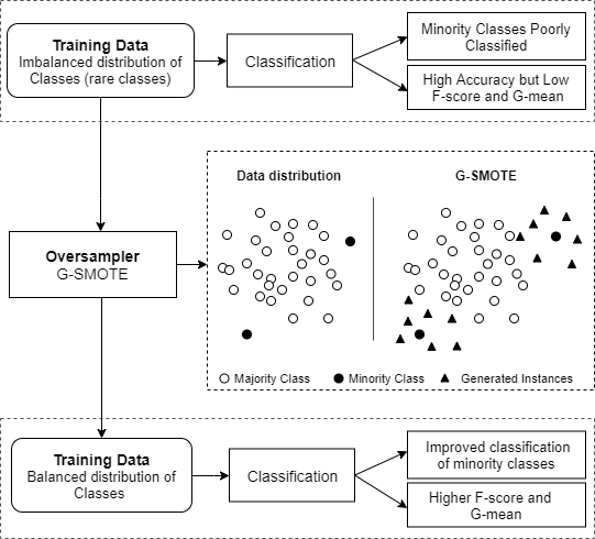
Oversampling algorithms attempt to even the distributions by generating artificial data for the minority class(es).
Hybrid approaches use both oversampling and undersampling techniques to ensure a balanced dataset.
In this paper, we compare the performance of various oversampling algorithms on EUROSTAT’s publicly available Land Use/Cover Area Statistical Survey (LUCAS) dataset [
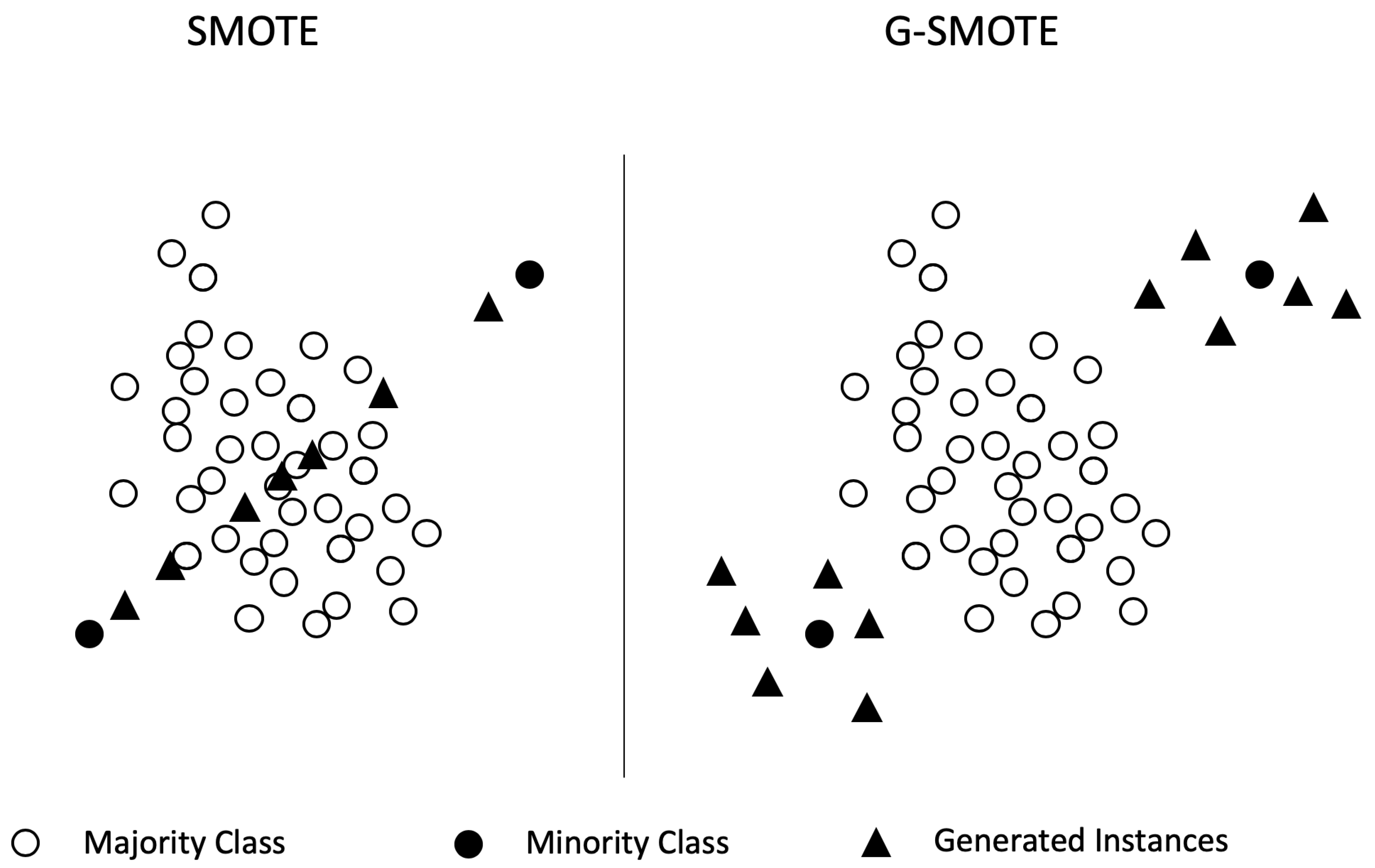
14] with Landsat 8 data. The experimental procedure included a comparison of five oversamplers using five classifiers and three evaluation metrics. Specifically, the oversampling algorithms were Geometric-SMOTE (G-SMOTE) [
15], the synthetic minority oversampling technique (SMOTE) [
16], Borderline-SMOTE (B-SMOTE) [
17], the adaptive synthetic sampling technique (ADASYN) [
18] and random oversampling (ROS), while no oversampling was included as a baseline method. Results show that G-SMOTE outperforms every other oversampling technique, for the selected evaluation metrics.
This paper is organized in five sections:
Section 2 analyzes the resampling methods,
Section 3 describes the proposed methodology,
Section 4 shows the results and discussion, and
Section 5 presents the conclusions drawn from this study.
3. Methodology
This section describes the evaluation process of G-SMOTE’s performance. A description of the study area, dataset, oversamplers, classifiers, evaluation metrics, and the experimental procedure is provided.
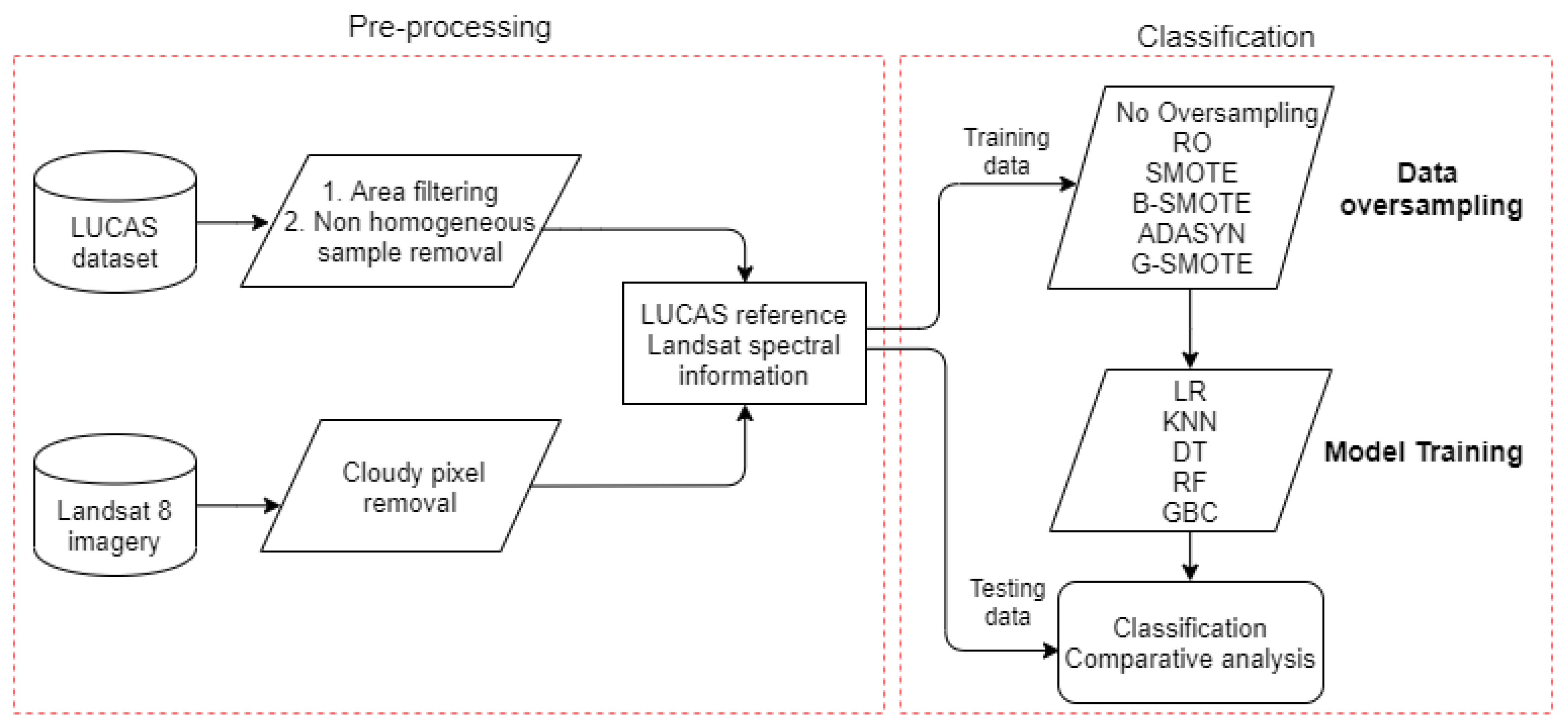
Figure 2 represents the flowchart of the steps applied in this experiment.
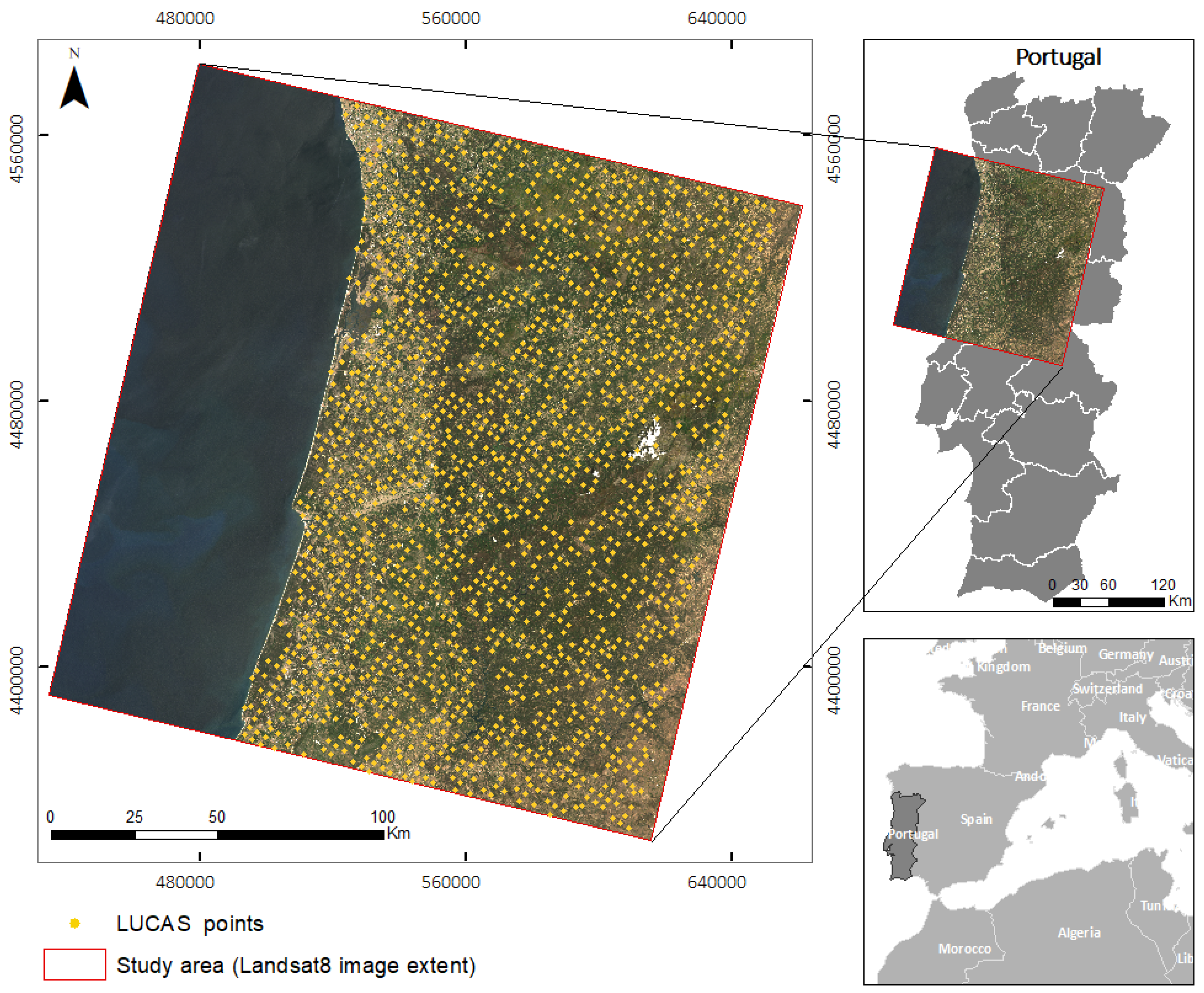
3.1. Study Area
The area of study was within north-western Portugal, corresponding to the area covered by the Landsat 8 image from track 204 and row 32, shown in
Figure 3. The area contains all eight main land cover types defined by LUCAS 2015: artificial land, cropland, woodland, shrubland, grassland, bare land, water, and wetlands.
3.2. Remote Sensing Data
The remotely sensed data includes eight images from the moderate-resolution Landsat 8 multi-spectral sensor. The images are Level-2 surface reflectance products (OLI/TIRS); one image was acquired each month from February to September 2015. The acquisition mode was descending. Data were pre-processed in order to remove pixels with cloud cover. Only bands 2, 3, 4, 5, 6, and 7 were used from each image. Accordingly, each reference point from the LUCAS dataset had 48 features, representing pixel values from each spectral band from each image.
3.3. LUCAS Dataset
The 2015 LUCAS data was used as reference data for both model training and validation. The LUCAS point label represents the corresponding land cover/use type within the radius of 1.5 m for homogeneous classes and a 20 m radius extent (“extended window”) for heterogeneous classes (e.g., shrubland), gathered by field observation and a very high-resolution photo interpretation [
6]. In order to reduce the risk of having Landsat pixel information represented wrongly in the field, we only kept points observed in situ from a close distance (<100 m). With the same objective we removed the points which had linear features in the observation (e.g., roads). This procedure was solely not applied to the class of “artificial land”, as this would have removed most parts of the samples. Furthermore, points with cloudy pixels in the Landsat data were also excluded. This way, 1694 out of 2060 LUCAS points were retained. This dataset contains eight classes that represent the main land cover types for the study area.
This pixel selection excluded a large number of unacceptable reference points, and we assumed the remaining ones to be suitable enough to represent the land cover type in a Landsat pixel coverage area of 30 × 30 m. Further, we surmised that classifiers are capable of overcoming the noise caused by pixels having mixed land cover representation if such pixels are still available in the dataset.
The number of samples per class and the imbalance ratio (IR), defined as the ratio of the number of samples for the majority class over the number of samples for any of the minority classes, is presented in
Table 1.
Table 2 presents a description of the LUCAS dataset, including information about the majority class C and the smallest minority class H to emphasize the imbalanced character of the dataset:
3.4. Evaluation Metrics
Amongst the possible choices existing for a classifier’s performance evaluation,
Accuracy, user’s accuracy (or
Precision) and producer’s accuracy (or
Recall) are the most common in LULC classification [
30,
31]. For a binary classification task, their calculation is given in terms of the true positives
, true negatives
, false positives
, and false negatives
[
30]. More specifically,
and
. For the multiclass case, the average value across classes is used, as explained below.
The LUCAS dataset is highly imbalanced, having a wide range of IRs for the different minority classes. Therefore, the use of the metrics above is not an appropriate choice since they are mainly determined by the majority class contribution [
32]. An appropriate evaluation metric should consider the classification accuracy of all classes. A simple approach for the multiclass case is to select a binary class evaluation metric; apply it to each binary sub-task of the multiclass problem, i.e., consider each class versus the rest; and finally, average its values. For this purpose,
F-score and
G-mean metrics were used as the primary evaluation methods, while
Accuracy is provided for discussion:
- -
The
Accuracy is the number of correctly classified samples divided by the sum of all samples. Assuming that the various classes are labeled by the index
c,
Accuracy is given by the following formula:
- -
The
F-score is the harmonic mean of
Precision and
Recall. The
F-score for the multiclass case can be calculated using their average per class values [
32]:
- -
The
G-mean is the geometric mean of
Sensitivity and
Specificity.
Sensitivity is identical to the
Recall while
Specificity is given by the formula
. Therefore, they are equal to the true positive and true negative rates, respectively. The
G-mean for the multiclass case can be calculated using their average per class values:
3.5. Machine Learning Algorithms
The main objective of the paper is to show the effectiveness of G-SMOTE when it is used on multiclass, highly imbalanced data of a remote sensing application and to compare its performance to other oversampling methods. Four oversampling algorithms were used in the experiment along with G-SMOTE. ROS was chosen for its simplicity. SMOTE was selected for being the most widely used oversampler. ADASYN and B-SMOTE were selected for representing popular modifications of the original SMOTE algorithm. Finally, no oversampling was applied as an additional baseline method.
For the evaluation of the oversampling methods, the classifiers logistic regression (LR) [
33], k-nearest neighbors (KNN) [
34], decision tree (DT) [
35], gradient Boosting classifier (GBC) [
36], and random forest (RF) [
37] were selected. The choice of classifiers was made according to the following criteria: learning type, training time, and popularity within the remote sensing community. All these algorithms were found to be computationally efficient and commonly used for the proposed task, with the exception of LR, which is rarely used in remote sensing applications [
2,
21].
3.6. Experimental Settings
In order to evaluate the performance of each oversampler, every possible combination of oversampler, classifier, and metric was formed. The evaluation score for each of the above combinations was generated through an n-fold cross-validation procedure with . Before starting the training of each classifier, and in each stage of the n-fold cross-validation procedure, synthetic data were generated using the oversampler, based on the training data of the folds, such that the resulting training set became perfectly balanced. This enhanced training set, in turn, was used to train the classifier. The performance evaluation of the classifiers was done on the validation data of the remaining fold, where , while D represents the dataset. The process above was repeated three times, and the results were averaged.
The range of hyperparameters used for each classifier and oversampler are presented in
Table 3:
3.7. Software Implementation
The implementation of the experimental procedure was based on the Python programming language, using the Scikit-Learn [
38], Imbalanced-Learn [
39], and Geometric-SMOTE libraries. All functions, algorithms, experiments, and results reported are provided at the GitHub repository of the project. Additionally, the Research-Learn library provides a framework to implement comparative experiments, also being fully integrated with the Scikit-Learn ecosystem.
5. Conclusions
In this paper we applied G-SMOTE, a novel oversampling algorithm, on a LULC classification problem, using a highly imbalanced, multiclass dataset (LUCAS). G-SMOTE’s performance was evaluated and compared with other oversampling methods. More specifically, ROS, SMOTE, B-SMOTE, and ADASYN were the selected oversamplers, while LR, KNN, DT, GBC, and RF were used as classifiers.
The experimental results show that using G-SMOTE can significantly improve the classification performance, resulting in higher values of F-score and G-mean. Therefore, readers should consider using G-SMOTE when accurately predicting the minority classes is of equal or higher importance compared to the accurate prediction of the majority class. Examples of the above case include the detection of land cover change and rare land cover type classification.
G-SMOTE can be a useful tool for remote sensing researchers and practitioners, as it systematically outperforms the currently widely used oversamplers. G-SMOTE is easily accessible to the users through an open source implementation.


