Article

Multilayer Soil Moisture Mapping at a Regional Scale from Multisource Data via a Machine Learning Method

1
Key Laboratory of Agricultural Remote Sensing, Ministry of Agriculture and Rural Affairs, Beijing 100081, China
2
State Key Laboratory of Information Engineering in Surveying, Mapping and Remote Sensing, Wuhan University, 129 Luoyu Road, Wuhan 430079, China
3
Collaborative Innovation Center of Geospatial Technology, 129 Luoyu Road, Wuhan 430079, China
4
State Key Laboratory of Water Resources and Hydropower Engineering Sciences, Wuhan University, Wuhan 430072, China
5
Changjiang River Scientific Research Institute, Changjiang River Water Resources Commission, Wuhan 430015, China
6
Guangxi Key Laboratory Cultivation Base of Water Engineering Materials, Guangxi Institute of Water Resources Research, Nanning 530023, China
*
Author to whom correspondence should be addressed.
Remote Sens. 2019, 11(3), 284; https://doi.org/10.3390/rs11030284
Submission received: 8 January 2019 / Accepted: 28 January 2019 / Published: 1 February 2019
(This article belongs to the Section Remote Sensing in Geology, Geomorphology and Hydrology)

Abstract

:
Soil moisture mapping at a regional scale is commonplace since these data are required in many applications, such as hydrological and agricultural analyses. The use of remotely sensed data for the estimation of deep soil moisture at a regional scale has received far less emphasis. The objective of this study was to map the 500-m, 8-day average and daily soil moisture at different soil depths in Oklahoma from remotely sensed and ground-measured data using the random forest (RF) method, which is one of the machine-learning approaches. In order to investigate the estimation accuracy of the RF method at both a spatial and a temporal scale, two independent soil moisture estimation experiments were conducted using data from 2010 to 2014: a year-to-year experiment (with a root mean square error (RMSE) ranging from 0.038 to 0.050 m3/m3) and a station-to-station experiment (with an RMSE ranging from 0.044 to 0.057 m3/m3). Then, the data requirements, importance factors, and spatial and temporal variations in estimation accuracy were discussed based on the results using the training data selected by iterated random sampling. The highly accurate estimations of both the surface and the deep soil moisture for the study area reveal the potential of RF methods when mapping soil moisture at a regional scale, especially when considering the high heterogeneity of land-cover types and topography in the study area.

Graphical Abstract

1. Introduction

Soil moisture controls the interaction between the land surface and the atmosphere in a climate system [1], including the exchange of water, energy, and carbon fluxes [2,3,4], by influencing the partitioning of the incoming radiant energy at the land surface into sensible and latent heat fluxes [5]. Generally, soil moisture represents the total amount of water restored in an unsaturated zone. Soil moisture in the root zone, usually 0~80 cm under the surface of a soil column, is critical to water management, such as irrigation and drainage in agriculture. Regional mapping of root zone soil moisture at an appropriate spatio-temporal resolution would, therefore, support more efficient water management. However, obtaining accurate information on multilayer soil moisture at a fine spatio-temporal resolution is challenging because of the high variability in soil moisture across spatial and temporal scales [6,7,8]. Soil moisture variability stems from the inherent heterogeneity of soil texture and structure, as well as variation in land-cover patterns, topographic features, and weather that vary as a function of scale [9,10,11].
Historically, soil moisture could only be measured with ground instruments, which include gravimetric methods [12], time-domain reflectometry [13], capacitance sensors [14], neutron probes [15], electrical resistivity measurements [16], heat-pulse sensors [17], and fiber-optic sensors [18]. The advantage of these techniques is that they are relatively mature and easily applied, and can provide soil moisture data at different soil depths. These measurements are considered as a ground truth. Over the past few decades, several networks for soil moisture monitoring have been installed to provide long-term measurements around the world. Some networks can be found in the International Soil Moisture Network (ISMN, http://ismn.geo.tuwien.ac.at/). However, due to the high variability of soil moisture and a network’s high maintenance and operating expenses, the sparseness of point measurement stations makes it challenging to map multilayer soil moisture as a spatially continuous variable at finer spatial resolutions.
Satellite remote-sensing observations from global imaging sensors offer considerable potential to characterize spatio-temporal patterns of soil moisture from the local to the global scale in a consistent, time- and cost-efficient manner [1,19,20,21,22]. Microwave observations are considered to be the most suitable for the retrieval of soil moisture based on the direct relationship between the soil dielectric constant and soil moisture [23,24]. Several passive and active microwave satellites have been developed to retrieve soil moisture, such as the Advanced Microwave Scanning Radiometer-EOS (AMSR-E) [25], the Soil Moisture and Ocean Salinity (SMOS) [26], the Soil Moisture Active Passive (SMAP) mission [21], and the Sentinel-1 [27]. Microwave remote-sensing techniques collect soil moisture data from the regional to the global scale; however, there are still two main limitations: low spatial resolution and limited penetration. The spatial resolution of the historical soil moisture data collected before 2014 (when Sentinel-1 was launched) is low (25~50 km) due to the constraints on antenna size and Earth orbits [26]. This coarse spatial resolution limits its application in many hydrological and agricultural studies at a regional scale. Moreover, only the surface soil moisture (the top ~5 cm of a soil column) can be retrieved based on remote-sensing data because of the limited microwave penetration depth [3,11,20].
The combination of optical and passive microwave remote-sensing data for surface soil moisture retrieval at a regional scale has been demonstrated in previous studies [28,29,30], among which spatial downscaling of remotely sensed surface soil moisture to 30 m~9 km resolution has been a popular way to obtain surface soil moisture at a finer spatial resolution. Excellent reviews on the current downscaling methods have been provided by [29] and [28]. These methods can be classified into six types: radar-based [31,32,33], radiometer-based [34], optical-based [35,36], soil surface attributes-based [37], data-assimilation-based [38], and machine-learning-based [39] downscaling methods. Their strengths and weaknesses have been well-listed in [28,29]. However, these methods are mainly developed for surface soil moisture retrieval by combining coarse spatial resolution soil moisture products and remote-sensing data from other satellite sensors (e.g., optical sensors) or auxiliary data (e.g., land-cover classes [30]). Peng [29] stated that there is a need for the synthesis of all available data sources to generate high-accuracy soil moisture products in a review of spatial downscaling of satellite remotely sensed soil moisture. In practice, however, root zone soil moisture estimation is more valuable than surface soil moisture in hydrological and agricultural applications.
Direct access to soil moisture in the root zone at a fine spatial resolution from remote sensing is still a serious challenge [40,41]. There are a few studies of high spatial resolution root zone soil moisture mapping at the regional scale, and they are generally based on the correlation between surface soil moisture and root zone soil moisture [40,42,43,44]. The exponential filtering method, for example, can only provide accurate estimates as long as the soil characteristics are relatively homogeneous throughout the soil column. Moreover, that the lag time varies with climatic conditions and soil moisture dynamics at different depths might have a negative influence on the performance of the model [40]. Thus, estimation of regional soil moisture in the root zone is still challenging due to the spatially varied topography, soil properties, climate conditions, etc.
Data assimilation has become a popular and effective way to estimate root zone soil moisture by assimilating in-situ and remotely sensed observations into deterministic models [45,46,47]. The data assimilation method, based on physical processes, improves our understanding of soil moisture variation and its interaction with the land–atmosphere boundary. One of the advantages of data assimilation modeling is that it can provide spatially continuous estimations of soil moisture at each depth and at a defined spatial resolution. However, soil texture exerts a greater degree of control over soil moisture evolution and the spatial distribution of moisture in soils at a deeper depth where influences from forcing and feedback at the land–atmosphere boundary are typically smaller [47,48]. Thus, when estimating deeper soil layers with different hydraulic properties from the surface soil layer, the data assimilation’s performance will significantly deteriorate [47]. Under these constraints, more observations at deeper layers with more detailed information about the soil, the land cover, and their interaction are necessary to improve the data assimilation’s performance when estimating soil moisture in the root zone [49,50]. However, this information is usually difficult to obtain at a regional scale [49,51]. Physiographic and geomorphic characteristics of most hydrologic systems are complicated, with a large degree of uncertainty in inputs, parameters, boundary conditions, and physical structures, which results in uncertainty and errors [52]. In addition, the application of physical-modeling-based methods is to some extent limited by the lack of required data and the expense of data acquisition.
To overcome the limitations of physical-modeling-based methods, machine-learning approaches provide an alternative to solve hydrological problems. They are based on an analysis of the data that characterizes the system under study with only a limited number of assumptions about the physical behavior of the system [53,54]. Although machine-learning approaches cannot physically describe the natural process, they have the advantages of dealing with noisy data from dynamic and nonlinear systems without numerous data requirements [55]. They allow us to solve numerical prediction problems, reconstruct highly nonlinear functions, perform classifications, group data, and build rule-based systems [56,57,58].
Recently, machine-learning approaches have been widely used to retrieve and downscale surface soil moisture from satellite observations [59,60,61,62,63,64,65]. However, the previous studies based on remote-sensing data mainly focused on downscaling or estimating surface soil moisture. To the best of our knowledge, there has, to date, been no reported use of machine learning for estimating root zone soil moisture at a fine spatial resolution based on remote-sensing data. Therefore, it will be interesting and meaningful to estimate root zone soil moisture via machine learning. It learns the relationship between soil moisture and all available information related to soil moisture variation, including topographical data, land-cover data, soil data, meteorological measurements, and remote-sensing observations.
In this study, a machine learning method was used to map both surface and root zone soil moisture (0~5, 25, and 60 cm depths from the surface of the soil column) at the regional scale with a 500-m spatial resolution based on data from multiple sources. The objectives of this study were: (1) to map multilayer soil moisture from multisource data at the regional scale via the random forest (RF) method, which is one of the machine-learning approaches; (2) to analyze the data requirement of this method by evaluating its performance with various training data sizes; (3) to examine the relative importance of the available variables and their variation in soil moisture estimation at different depths; and (4) to evaluate the performance at both a spatial and a temporal scale.

2. Materials and Methods

2.1. Study Area

Oklahoma, in the United States of America, lies partly in the Great Plains between latitudes 33°37’ N and 37° N and longitudes 94° 26’ W and 103° W (Figure 1). It is in a humid subtropical region. Most of the state lies in an area known as Tornado Alley, which is characterized by frequent interaction between cold, dry air from Canada, warm to hot dry air from Mexico and the Southwestern United States (U.S.), and warm, moist air from the Gulf of Mexico. The average annual precipitation increases sharply from west to east, ranging from about 431.8 mm in the far western panhandle to about 1422.4 mm in the far southeast. Oklahoma is a region with a highly variable climate, geology, and topography and diverse plant communities [66].

2.2. Data Collection and Pre-Processing

The interacting factors that are closely related to soil moisture and available at a regional scale are shown in Figure 2, based on the mechanisms proposed by [67]. These factors influence or reflect the variation of soil moisture contents. Among these parameters, many of them are strongly interlinked.
To estimate multilayer soil moisture, the variables used to estimate soil moisture in this study include SMOS products (surface soil moisture, vertically and horizontally polarized brightness temperature), the normalized difference vegetation index (NDVI), the land surface temperature (LST), the actual and potential evapotranspiration (ET and PET, respectively), precipitation estimation from the Tropical Rainfall Measuring Mission (TRMM), Precipitation Analysis (TMPA) products, elevation, slope, net radiation (NR), soil property data, and the temperature/vegetation dryness index (TVDI), which are shown in boldface in Figure 2 and described in detail in Table 1. Albedo data were used in a preliminary test, but were not included in this study, as they had little impact on the result in this study and also reduced the number of data records due to missing data.

2.2.1. SMOS Products

The European Space Agency (ESA)’s SMOS mission, which has been operating since November 2009, is the first satellite dedicated to measuring surface (~5 cm depth) soil moisture and ocean salinity. SMOS L3 ascending products for the period of 2010–2014 in ~25 km cylindrical projection were used in this study, including soil moisture and horizontally and vertically polarized brightness temperature data at an incident angle of 42.5° with a 1~3 day temporal resolution. These data were downloaded from CATDS (Centre Aval de Traitement des Données SMOS, http://www.catds.fr/). The ascending product rather than the descending product was selected in this study because the thermal equilibrium and near-uniform conditions in the surface soil layer and overlying vegetation required for soil moisture retrieval are more likely to be reliable at 6 a.m. than at 6 p.m [68].

2.2.2. MODIS Products

The Moderate Resolution Imaging Spectroradiometer (MODIS) products used in this study include: 8-day composite 500-m Global Evapotranspiration data (MOD16A2, Version6), Daily and 8-day composite 1-km LST data (MOD11A1 and MOD11A2, Version6), and 500-m surface reflectance data (MOD09GQ and MOD09Qq, Version6) from Terra satellites for the period of 2010–2014. The study area covers two MODIS tiles (h09v05 and h10v05). The data were downloaded from NASA’s Earth Observing System Data and Information System (EOSDIS; http://reverb.echo.nasa.gov/reverb/). The nominal equatorial passing time of Terra is around 10:30 a.m. and p.m. local solar time. The Terra MODIS instruments collectively provide two daily LST observations that are available for analysis, which enable analyses of day, night, and day/night LST differences (Lstday, Lstnight, and Lstgap, respectively).
The NDVI was calculated from the surface reflectance products (Equation (1)). ET and PET were obtained from the Global Evapotranspiration data. The ratio of ET to PET (ET/PET) was calculated from ET and PET. ET-related variables were only used in the 8-day soil moisture estimation, as MODIS ET products are only available for 8-day composition estimation rather than daily retrieval.
N D V I = ρ N I R ρ R e d ρ N I R + ρ R e d
where ρ N I R and ρ R e d are near-infrared and red reflectance, i.e., MODIS band 2 and band 1, respectively.

2.2.3. In-Situ Data

The ground-measured daily soil moisture (at 0~5 cm, 25 cm, and 60 cm) data from 2010 to 2014 in Oklahoma were obtained from the Oklahoma Mesonet website (www.mesonet.org/). The Oklahoma Mesonet is a jointly owned environmental monitoring network of the University of Oklahoma (OU) and Oklahoma State University (OSU), operated from the Oklahoma Climatological Survey. This network, which has been in operation since 1994, measures weather and soil conditions at 120 surface stations across Oklahoma. The daily soil moisture is based on the 24-hour average soil moisture at different depths at each Mesonet site. Quality assurance (QA) procedures are conducted daily on the Oklahoma Mesonet data using a combination of automated routines and human inspection to determine erroneous observations and repair sensors [69].

2.2.4. Other Data

The TRMM TMPA products provide precipitation for the spatial coverage of 50° N–S at the 0.25° × 0.25° latitude–longitude resolution from the wide variety of modern satellite-borne precipitation-related sensors [70]. TRMM 3B42, the TMPA product, from 2010 to 2014 was used in this study. Multiple time scale precipitation variables based on TRMM observations were calculated (Table 1). Additional auxiliary data to improve the estimation performance include: elevation, net radiation (NR), and soil property data.
Shuttle Radar Topography Mission (SRTM) one Arc-Second Global elevation data, published in 2014, was downloaded from the Earth Explorer website (https://earthexplorer.usgs.gov/). It offers worldwide coverage elevation data at a resolution of one arc-second (30 meters) within a 50° north and a 50° south latitude. Slope data were calculated from the elevation data.
The net radiation data for 2010–2014 in the study area were obtained from the Earth Observatory website (https://earthobservatory.nasa.gov/global-maps). The measurements were made by the Clouds and the Earth’s Radiant Energy System (CERES) sensors on the NASA Terra and Aqua satellites.
The soil property data of clay, silt, and sand content from the Harmonized World Soil Database V1.2, published in 2009, were used in this study (Figure 3). The Harmonized World Soil Database is a 30-arc-second raster database with over 15,000 different soil mapping units that combines existing regional and national updates of soil information worldwide. This allows for soil components and attributes to be seen at a high level of spatial resolution (http://www.fao.org/soils-portal/soil-survey/soil-maps-and-databases/en/).
A simplified temperature/vegetation dryness index (TVDI) [67] was used to estimate the daily soil moisture in this study. The TVDI is related to surface soil moisture due to changes in thermal inertia and evaporative control of net radiation partitioning (energy balance) [67], and is widely used to evaluate soil moisture status [71,72,73]. The TVDI from 2010 to 2014 in the study area was calculated based on an empirical parameterization of the relationship between land surface temperature (Ts) and NDVI (a triangular Ts/NDVI space, see [67]) (Equation (1)).
T V D I = T s T s m i n a + b × N D V I T s m i n
where Ts is the observed LST at a given pixel, Tsmin is the minimum LST in the Ts/NDVI space (on the wet edge), NDVI is the observed NDVI value calculated from MODIS surface reflectance data, and a and b are parameters defining the dry edge modeled as a linear fit to the data (Tsmax = a + b*NDVI).

2.2.5. Data Pre-Processing

Data from multiple sources have different spatial and temporal resolutions. All of the variables were resampled to 500 m × 500 m resolution to estimate the 500 m × 500 m soil moisture. For the 8-day average soil moisture estimation, 8-day composite LST and surface reflectance data that were totally cloud-free in the study area were used from the day of year 1 to 361 (e.g., 1, 9, 17… 361) in 2010–2014 (Table A1), and the other variables were integrated into the same time scale. For the daily soil moisture estimation, only cloud-free days of the whole study area (Table A2) in Oklahoma were selected from 2010 to 2014. Daily observations of the variables were collected on the selected days.
The reason for only selecting totally cloud-free images in the study area is that all data from 2010 to 2014 could be possibly selected as training data for analysis. Selecting totally cloud-free days generally ensured that observations from satellite imagery were available for all of the stations, that the data from different stations were observed at the same time, and that the number of observations at each station was nearly the same during the study period, which permitted a comparison of the estimation results for different stations. As a result, daily observations were much less than the 8-day composite data, as 8-day composite products were collected on the cloud-free days for each pixel for the 8-day period.
Observation errors in the variables may affect the accuracy of soil moisture estimation. Only pixels flagged as high quality in the quality-assurance data were retained. Low-quality data in the MODIS variables were eliminated because remote-sensing-based LST and NDVI estimates are strongly influenced by error, such as error caused by cloud cover, large sensor viewing angles, and uncertainties in surface emissivity [74].

2.3. Methods and Application

2.3.1. The Random Forest Method

The random forest (RF) method is one of the machine learning approaches. It was used to map the regional soil moisture. It is an ensemble machine learning technique developed to improve the classification and regression tree (CART) methods that combine tree predictors [75]. A regression tree represents a set of hierarchically organized conditions or restrictions that are successively applied from a root to a leaf of the tree. Two parameters must be optimized in RF: the number of regression trees (ntree; the default value is 500 trees) and the number of input variables per node (mtry; the default value is 1/3 of the total number of variables). To model the relationship between soil moisture and available variables, a set of training input–output pairs were given (i.e., the calibration data set).
To find the optimal ntree and mtry values, mtry and ntree were optimized based on the root mean square error (RMSE) of the calibration using the training dataset [76,77]. The ntree values from 1000–9000 with intervals of length 1000 were tested, while mtry was tested from 1 to 26 with a single interval. The ntree and mtry values that yielded the lowest RMSE were selected.

2.3.2. The RF Method’s Application

In order to investigate the estimation accuracy of the RF method at both a spatial and a temporal scale, two independent experiments, a year-to-year experiment and a station-to-station experiment, were conducted in this study. The framework design is shown in Figure 4.
In the year-to-year experiment, the 5 cm, 25 cm, and 60 cm 8-day average soil moisture (Y05_8day, Y25_8day, and Y60_8day, respectively) and the daily soil moisture (Y05_daily, Y25_daily, and Y60_daily, respectively) were estimated. It estimated the soil moisture at the stations at a randomly selected time using the ground-measured soil moisture at the corresponding data layer observed from the same stations but at other times as training data, i.e., the stations to be estimated in the test dataset are all the same as those in the training dataset.
In the station-to-station experiment, the 5 cm, 25 cm, and 60 cm 8-day average soil moisture (S05_8day, S25_8day, and S60_8day, respectively) and the daily soil moisture (S05_daily, S25_daily, and S60_daily, respectively) were estimated. It estimated the soil moisture of randomly selected stations using the ground-measured soil moisture at the corresponding data layer observed from other stations as training data, i.e., the stations to be estimated in the test dataset are all not included in the training dataset.
In Section 3 (Results), in order to demonstrate the estimation results of the proposed method, the 5-, 25-, and 60-cm depth soil moisture of all available stations in 2010 and 2012 was taken as the training data and that of all available stations from 2013 to 2014 was taken as the test data to estimate the 8-day average 5-cm, 25-cm, and 60-cm depth soil moisture and daily 5-cm, 25-cm, and 60-cm depth soil moisture. The 5-, 25-, and 60-cm depth soil moisture of a randomly selected two thirds of all stations from 2010 to 2014 was taken as the training data and that of another one third of all stations from 2010 to 2014 was taken as the test data to estimate the 8-day average 5-cm, 25-cm, and 60-cm depth soil moisture and the daily 5-cm, 25-cm, and 60-cm depth soil moisture.
Then, in Section 4 (Discussion), in order to analyze and evaluate the data requirement, spatial and temporal variation in the model’s performance, random sampling, and an iteration method were used to avoid overtraining and chance factors.
As for the year-to-year estimation, random sampling was run for 100 iterations for each estimation of soil moisture to select the data from one third, two thirds, and all stations as data pools, from which 1000 data records were selected from the corresponding pools as the test data, and then 100~20,000 data records were randomly selected from the corresponding remaining data as the training data, for each iteration. In each iteration of estimation, the stations included in the training data and the test data were the same. The final estimation accuracy of the RMSE was averaged from the accuracy of 100 iterations to control for random effects.
The process for estimating the daily soil moisture was similar to that for estimating the 8-day average soil moisture, but fewer data records were available. A total of 100~3000 and 300 data records were selected for the training data and the test data, respectively, for the year-to-year daily estimation. In the station-to-station daily estimation, for each iteration, data from one year, three years, and all five years were randomly selected to be the data pools, and then the data from 20 randomly selected stations were selected from the pool of the selected one year, three years, and five years of data as the test data. Data from 10~80 stations were randomly selected as the training data from the remaining data in the data pool. The final accuracy of each estimate was averaged by the estimation accuracy of 100 iterations to control for random effects.
In addition, caution was taken to avoid overtraining. The RF method is not sensitive to noise or overtraining, as resampling is not based on weighting [78]. First, random resampling and iteration methods were used to make the value pattern of the training data similar to that of the test data. Second, more than 20 variables were used in the RF method, as overtraining is less likely to occur with more variables. Moreover, the training data set’s size was large; the effect of occasional overtraining can be minimized if a stable relationship between estimation accuracy and the training data set’s size can be obtained.

2.3.3. Evaluation Method

The statistical relationship between estimated soil moisture and ground-measured soil moisture was analyzed in this study. A simple random sampling method was used to divide the calibration and validation datasets. Five statistical parameters, including the slope and determination coefficient (R2) of a fitted line, the bias (Equation (3)), the root mean square error (RMSE) (Equation (4)), and the coefficient of variation (CV) of the RMSE (Equation (5)) to the average number of observations, were used to evaluate the estimation performance.
b i a s = i = 1 n ( y e , i y o , i ) / n
R M S E = i = 1 n ( y e , i y o , i ) 2 / ( n 1 )
C V = R M S E / i = 1 n y o , i
where y e , i is the i th estimated soil moisture value from the remote sensing data, and y o , i is the corresponding i th ground-observed soil moisture value.
The reduction in mean square error (MSE) (Equation (6)), when permuting a variable, was used as the random forest importance criterion in this study [75,79]. Standardized importance was calculated by changes in MSE and it was standardized by defining the importance value of SMOS_SM as 1.
M S E = i = 1 n ( y e , i y o , i ) 2 / n

3. Results

3.1. Multilayer Soil Moisture Mapping over Oklahoma

The 8-day average and daily soil moisture mapping at the depths of 5, 25, and 60 cm with a spatial resolution of 500 m was achieved using the RF method in this study. Figure 5 shows the estimated 8-day average and daily soil moisture maps within the year-to-year experiment using data from 2010 to 2012 as training data at the representative times of 11–18 December 2013 and 11 December 2013, respectively, using the data from 2010 to 2012 as training data.
The soil moisture estimated using the RF method has a higher spatial resolution with more detailed spatial information than the SMOS soil moisture data. With the increase in depth, the spatial similarity of the soil moisture between SMOS and the estimations deteriorated. SMOS instruments have a limited observational capacity in deep soil due to the limited penetration depth (<5 cm) of the microwave. However, there were few differences in the spatial pattern between the 8-day average and daily soil moisture estimations from both SMOS and the RF method at each depth, since little precipitation was observed from 11 to 18 December 2013. The total precipitation estimated by the TRMM satellite was only 0.64 mm during this period. Moreover, the estimated 8-day average soil moisture from the RF method was more continuous at the spatial scale, as there were no clear demarcation lines of the SMOS footprint, which are clearly visible in the estimated daily soil moisture maps.

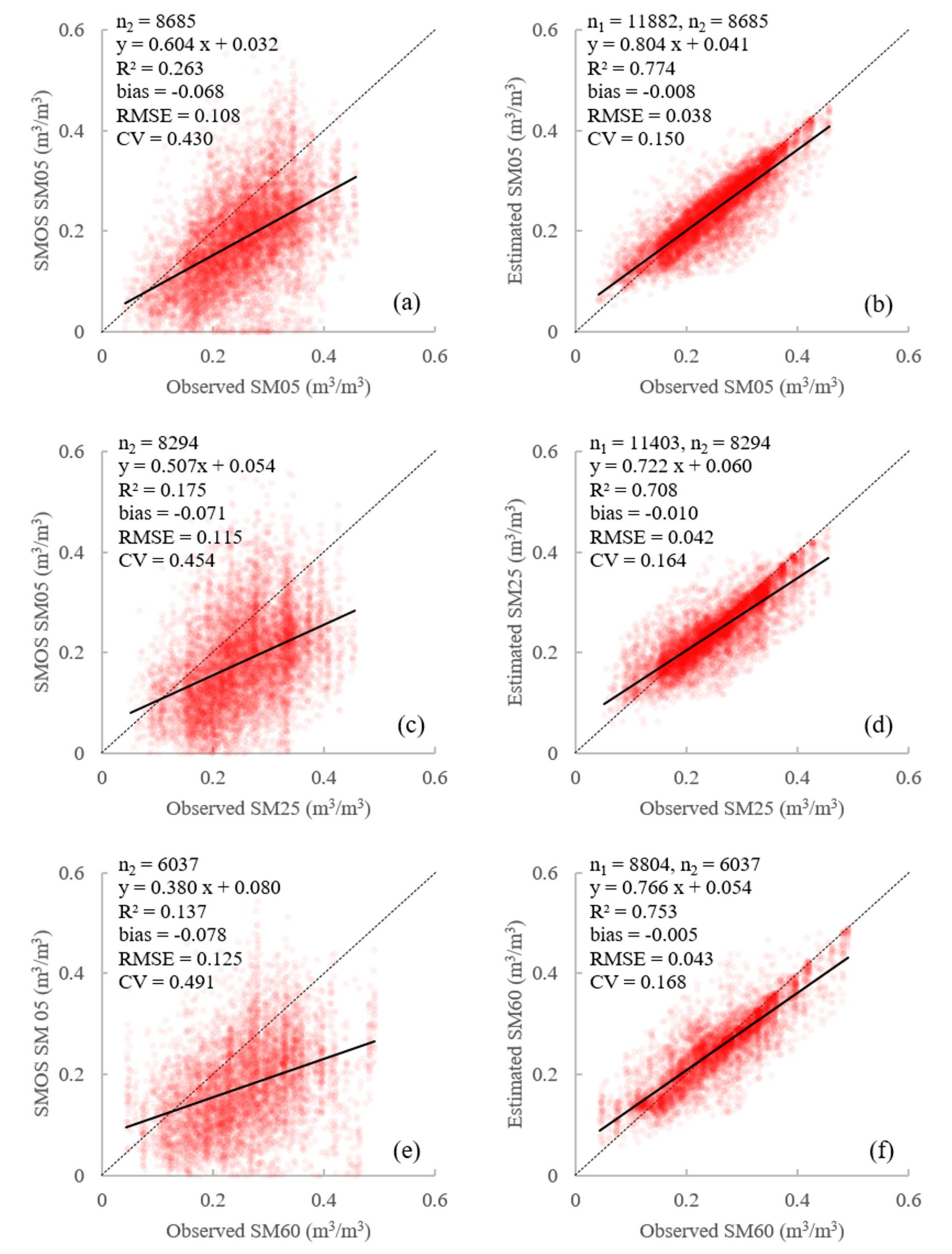
3.2. Year-to-Year Estimation

In the year-to-year estimation, quantitative assessments were used to compare the estimated soil moisture at each depth and the corresponding ground-measured soil moisture at the observation stations for the years 2013–2014. Figure 6 and Figure 7 show the scatter plots of the ground-measured 8-day average and the daily soil moisture against the SMOS soil moisture and the estimated soil moisture.
As shown in Figure 6, the estimated 8-day average had high accuracy (RMSE = 0.038~0.043 m3/m3) and reproduced the spatial pattern well (slope = 0.804, 0.722, and 0.766). The accuracy and spatial pattern reproduction of the daily estimated soil moisture were inferior to that of the 8-day average estimation results in terms of slope, R2, RMSE, and CV (Figure 7). One reason for this is that the size of the training data set for the 8-day average estimation was about 4 times that for the daily estimation. In general, a larger size of the training data set would result in better estimation performance [77]. The different overpass times of the daily data from multiple sources might be another reason, which might also be the reason why a more stable relationship between the soil moisture and the available variables could be observed for the 8-day estimation but not the daily estimation. Nevertheless, the accuracy of both the 8-day average and daily soil moisture estimates at each depth was significantly higher than the SMOS observations in terms of all statistical parameters.
The estimation accuracy varied with soil depth. The correlation between SMOS observations and the observed soil moisture was higher at the 5-cm depth than that at the 25-cm depth or the 60-cm depth. The reason for this is that the microwave band (1.41 GHz) of SMOS can only retrieve surface soil moisture information, and does not penetrate to deep soil layers. Similarly, the estimation accuracy was also higher at the 5-cm depth than that at the 25-cm depth or the 60-cm depth in terms of all statistical parameters, for both the 8-day average and daily soil moisture estimations (Figure 6 and Figure 7). Most of the inputs only reflect the land-surface properties; little information directly relates to deep soil moisture.
The differences in estimation accuracy between the 25-cm depth and the 60-cm depth in terms of the RMSE and the CV were smaller in the 8-day average estimation than those in the daily estimation. The 8-day average soil moisture estimated at a 60-cm depth delivered a better reproduction of the spatial pattern than that at a 25-cm depth in terms of slope and R2, but presented lower accuracy in terms of RMSE and CV. In the daily estimation, similar results were observed.
The data were imbalanced, as the in-situ observations have far fewer data records at a low value (<0.1 m3/m3) of soil moisture, and estimation in extremely dry conditions is apt to be overestimated, especially at the 25-cm depth.

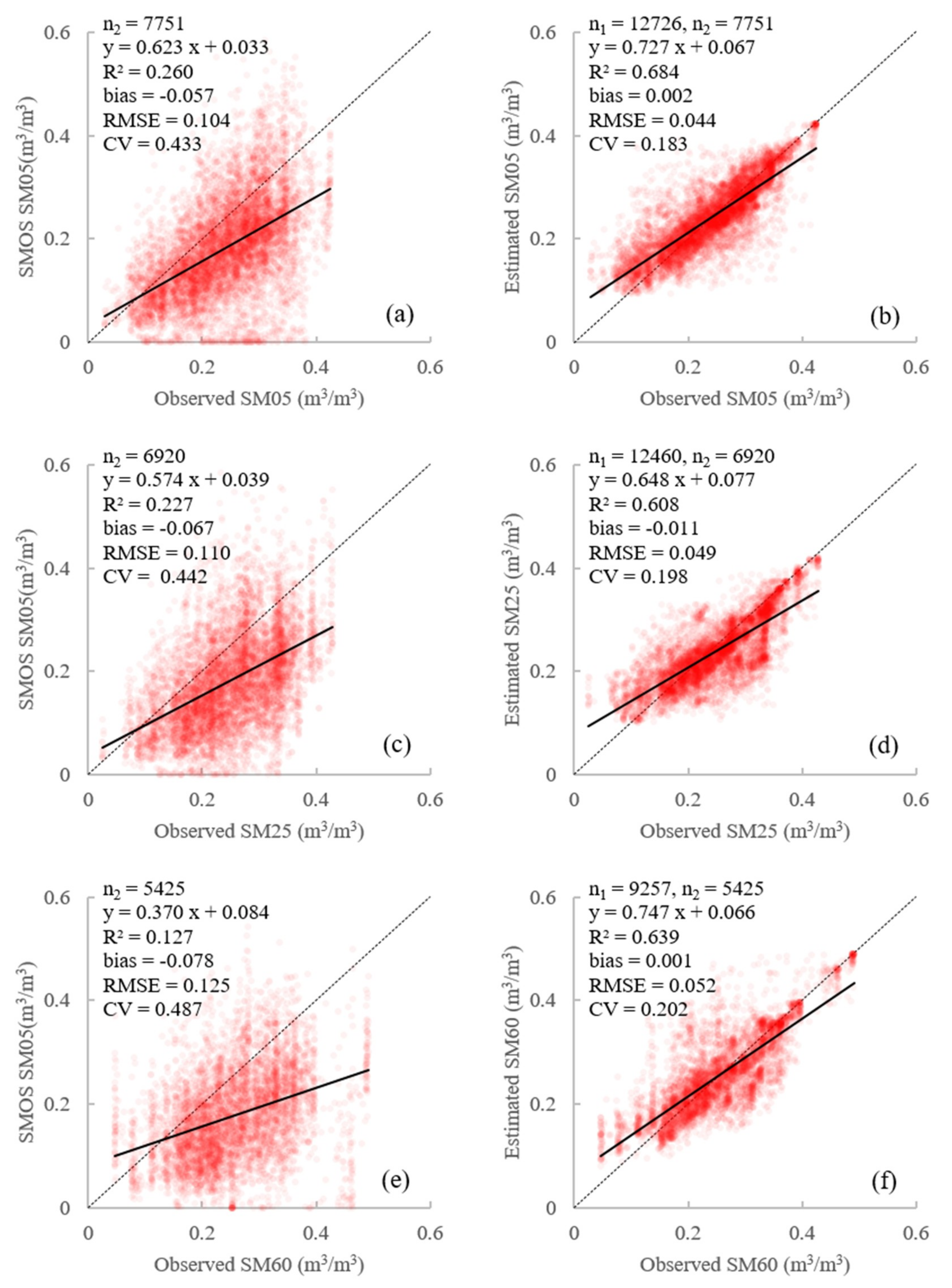
3.3. Station-to-Station Estimation

The year-to-year estimation experiment demonstrated the potential of the RF method to estimate soil moisture using ground-measured soil moisture observed in other years as training data. One issue is whether the relationship between soil moisture and the available variables in known stations can be applied to other sites with no ground-measured training data, which needs to be further studied. Thus, to verify the reliability of the RF method to estimate soil moisture at unknown sites, randomly selected data from two thirds of all stations were used as training data. Data from the other one-third of all stations were used as test data to conduct the station-to-station experiment.
Combining the available data from multiple sources using the RF method delivered higher accuracy than SMOS when estimating the station-to-station soil moisture. As shown in Figure 8 and Figure 9, the RF method was reliable when estimating the soil moisture for unknown areas in terms of slope, R2, bias, RMSE, and CV, although the result of the station-to-station estimation was inferior to that of the year-to-year estimation. Similar to the year-to-year estimation, with the increase in soil depth, the correlations between the SMOS/RF-derived soil moisture and the observed data deteriorated and the estimation accuracy decreased in terms of all statistical parameters. In addition, due to the soil moisture data imbalance, estimation under extremely dry conditions was apt to be overestimated, especially at the 60-cm depth (RMSE >0.05 m3/m3, CV >0.2).

4. Discussion

The year-to-year and station-to-station experiments showed that the RF method was able to obtain accurate soil moisture estimations in the study area by combining ground-measured and remotely sensed data. In the year-to-year experiment, the stations included in the test data set and the training data set were the same, but the performance varied with the quantities of training data records and included stations. In the station-to-station experiment, it is unclear how many data records and stations with ground-measured soil moisture are required to achieve a reasonable estimation accuracy. The contribution and importance of the considered inputs must be quantified. The spatial pattern of the accuracy of soil moisture estimates for individual stations must be analyzed. The variation in performance of this method at the temporal scale and the spatial scale must be considered. The uncertain sources affecting the RF method must be analyzed. In the following subsections, these issues are discussed.

4.1. Data Requirements in the Year-to-Year Soil Moisture Estimation

To reveal the influence on the estimation accuracy of the quantities for all data records and for the average data records of individual stations in the training data set, the performance of the RF method with different quantities of data records and observation stations in the training data set was collected. The average result was derived from 100 iterations. Figure 10 shows the estimation accuracy changing with included stations and data records in the training data set for the year-to-year soil moisture estimation.
As shown in Figure 10, the RMSE of the estimated 8-day average and daily soil moisture at each depth decreases as the quantity of data records in the training data set increases, since the training data set’s size is an important factor that can affect the results of the RF method’s estimation accuracy [77]. When all available stations were included in the training data set and the testing data set, the RMSE of the estimation decreased rapidly when the number of data records was less than 2000 and 700 for the 8-day average soil moisture estimation and the daily soil moisture estimation, respectively, while it decreased slowly when the number of data records in the training data set was more than 2000 and 700, respectively. Accordingly, 2000 and 700 data records are necessary for training data with about 120 stations for the 8-day average soil moisture estimation and the daily soil moisture estimation, respectively.
In contrast to the 8-day average soil moisture estimation, the daily estimation needed less training data when the curve in Figure 10 became flat, although the final accuracy of the daily soil moisture estimation was slightly lower than that of the 8-day average soil moisture estimation at each depth (Figure 10). This is probably because the daily variables, such as the daily in-situ soil moisture observation, the daily SMOS soil moisture and brightness temperature, and the LST, have a larger variation range than the 8-day composite data. As a result, daily soil moisture estimation by the RF method requires less training data but has a large variation range when capturing the relationship between estimated soil moisture and variables from multiple resources.
For both 8-day average and daily soil moisture estimation, with the same number of data records in the training data set, a higher accuracy was achieved when fewer stations were included. Fewer data records were required for an estimation with fewer stations than for an estimation with more stations. For example, as shown in Figure 10a, with randomly selected data from one third (40 stations) and two thirds (80 stations) of all stations, and all stations (120 stations) as training data, 8000, 14,000, and 20,000 data records are required, respectively, to obtain a similar accuracy to the 5-cm depth, 8-day average soil moisture results (about 200, 175, and 167 data records from each station for the three conditions, respectively). That is, including more data records from a corresponding station in the training data set will increase the estimation accuracy at this station more than when using data from other stations.

4.2. Data Requirements in the Station-to-Station Soil Moisture Estimation

The data requirement for the year-to-year estimation was discussed in Section 4.1; however, in most situations, we need to estimate the soil moisture of the locations where there is no ground equipment for soil moisture measurement using remote-sensing data and ground-measured soil moisture from other observation stations. Figure 11 shows the estimation accuracy changing with included stations and data records in the training dataset for the station-to-station soil moisture estimation.
As shown in Figure 11, the estimation error in the station-to-station estimation decreases with the increase in the number of data records and included stations in the training data set. A larger quantity of data records in this subsection means that data for a longer period were included (e.g., one year, three years, and five years). The estimation accuracy significantly increased when the number of stations participating in the training data increased, but the accuracy improved slightly with an increase in the number of data records from individual stations for the 8-day average soil moisture estimation.
This was probably because there were more data records available for the 8-day average soil moisture estimation than for the daily soil moisture estimation in a single year. Accordingly, in station-to-station soil moisture estimation for unknown stations, the quantity of observation stations included in the training data set increases the accuracy more than the quantity of data records from individual stations if the number of records from individual stations is not too small and the stations are evenly distributed.
In addition, compared to both the 8-day average and the daily 5-cm and 25-cm depth soil moisture estimation, the difference in the 60-cm depth soil moisture estimation accuracy with different numbers of training data records was less pronounced. The temporal and spatial variations in the 60-cm depth soil moisture were less significant than those in the 5- and 25-cm depth soil moisture. As a result, the temporal and spatial patterns of the 60-cm depth soil moisture were easier to estimate with even fewer training data records.

4.3. Factor Importance

Figure 12 shows the relative importance of variables in both the 8-day average and the daily soil moisture estimation by defining the importance of the SMOS soil moisture data as 1. Generally, the importance of variables derived from the SMOS satellite (Horizontally polarized brightness temperature (BTH), Vertically polarized brightness temperature (BTV)) decreased with an increase in soil depth because of the limited penetration depth (0~5 cm) of the used microwave band, which is also the reason why the correlation between the SMOS-derived and the ground-observed soil moisture decreased with an increase in soil depth (Figure 6, Figure 7, Figure 8 and Figure 9).
The impact of topographic features, such as elevation, slope, and soil properties, increased with an increase in soil depth, especially in the daily soil moisture estimation, as the variability of the surface soil moisture usually has a close connection to the upper boundary condition, while the variation in deep soil moisture is mainly controlled by soil properties and the topography [47,48]. As shown in Figure 13, the 5-cm depth soil moisture fluctuated due to the varied upper boundary condition, while the variation in the deep soil moisture is usually less sensitive than in the shallow soil.
The importance of precipitation from the TRMM was not significant compared to other factors probably due to its coarse spatial resolution and the estimation error in TRMM precipitation products. There was no significant difference among the importance of the three precipitation-related variables in the estimation of the 8-day average soil moisture. The importance value of five precipitation-related variables in the daily soil moisture estimation varies. In addition, Figure 12 shows that the importance of precipitation on previous days or for a longer period tends to be more significant, as the soil moisture status is strongly correlated to previously accumulated precipitation and the time lag between precipitation and an increase of soil moisture, especially for deep soil moisture.
In the 8-day average soil moisture estimation, the importance of NR, ET, and ET/PET increased with the increase in soil depth, which indicated that the water demanded for evapotranspiration might come from a deeper soil layer and is taken up by plant roots.
As to MODIS-derived variables (Lstday, Lstgap, and NDVI), there was no obvious trend with the increase in soil depth for the 8-day average soil moisture estimation. In the daily soil moisture estimation, the importance of Lstday decreased with the increase in soil depth. This is because the correlation between Lstday and soil moisture at the surface soil layer was higher than that in deeper layers and the daily variables that reflect the near-real-time conditions could capture this relationship more completely than 8-day average observations.

4.4. Spatial Pattern

Figure 14 shows the spatial pattern of estimation accuracy of 8-day average and daily soil moisture at different depths in the year-to-year and station-to-station experiments. Though daily soil moisture has a relatively lower estimation accuracy than 8-day average soil moisture, high accuracy (RMSE <0.05 m3/m3) was achieved at most observation stations for both the 8-day average and the daily estimations, which indicates that the RF method is a reliable way to estimate multilayer soil moisture. In the crop-planting area (shown in Figure 1), however, relatively larger RMSEs were observed, probably because human activities, such as irrigation and drainage, play a significant role in the soil water balance in crop areas; however, they were not considered in this study.

4.5. Seasonal Pattern

Figure 15 shows that the estimation accuracy of both the 8-day average and the daily soil moisture estimations varied with the season. Both the 8-day average and the daily soil moisture estimation at each depth tended to have relatively lower accuracies in summer and autumn than in other seasons in terms of CV. The reason for this was that the ratio of data records with a low value in the training data was low; however, most of the low values took place in summer and autumn in the study area. The RF method has a limited capacity to estimate soil moisture with small values due to the limited number of data records with a low value in the training data. The soil moisture in spring and winter tends to be high. As a result, a lower CV was observed in spring and winter in both the 8-day average and the daily soil moisture estimations.

4.6. Error and Uncertainty Analysis

Several possible sources of errors affecting the performance of the RF method must be noticed. First, remaining clouds (pixel and sub-pixel) of the optical and infrared observations from satellites negatively affect the model’s performance. Most undetected cloud-contaminated LST outliers occur in cloud edges, and a large proportion of the pixels with higher errors occur near identified clouds [80]. In addition, other observations (e.g., SMOS products, TRMM data, MODIS products, soil properties, and in-situ soil moisture observations) also suffer from uncertainty due to blemishes on instruments and imperfect algorithms. Mismatched observation times in the available data from multiple sources can also lead to errors in estimated soil moisture. Moreover, overestimation of low soil moisture (<0.1 m3/m3) due to data imbalances is one of the limitations of the RF method, as fewer data records of low soil moisture observations were included in the training data set, especially when estimating soil moisture under extremely dry summer and autumn conditions.

5. Conclusions

In this study, based on satellite imagery and ground-measured soil moisture data, both 8-day average and daily soil moisture at multiple depths (5, 25, and 60 cm) were estimated by the RF method in Oklahoma, U.S. from 2010 to 2014. The efficiency of the RF method displayed no indications of overtraining, and the results of this study are promising. In the year-to-year experiment, the estimation accuracy of soil moisture at different depths varied from 0.038 to 0.043 m3/m3 and from 0.042 to 0.050 m3/m3 for the 8-day average and the daily estimated soil moisture, respectively. In the station-to-station experiment, the estimation accuracy varied from 0.044 to 0.052 m3/m3 and from 0.045 to 0.057 m3/m3 for the 8-day average and the daily estimated soil moisture, respectively. The 8-day average soil moisture estimation has a higher accuracy than the daily estimations for the reason that the larger size of the training data set for the 8-day average soil moisture estimation resulted in better estimation performance.
The accuracy of soil moisture estimation varied with space, time, and soil depth. On the spatial scale, the stations that were located in crop-planting areas tended to have a lower estimation accuracy of soil moisture. Taking information on agricultural practices into consideration (e.g., irrigation and drainage) might improve the performance of soil moisture estimation in crop-planting areas. On the temporal scale, a lower estimation accuracy of both the 8-day average and daily soil moisture at each depth was observed in summer and autumn due to a lack of data records with low soil moisture values. On the vertical scale, with the increase in soil depth, the estimation accuracy decreased due to the limited amount of information observed at the deep soil layer. To improve the accuracy at the deep soil layer, more information, such as the groundwater level, more detailed soil property information at a finer spatial resolution, and other factors that affect the estimation accuracy need to be included to improve the performance of the method proposed in this study.
The SMOS products, topography, and soil properties were important for the soil moisture estimation. SMOS products provide average information of land surface for each pixel with coarse spatial resolution, and significantly contribute to the surface soil moisture estimation. However, with an increase in soil depth, the importance of SMOS products decreases due to the limited penetration of the remote-sensing equipment. However, the importance of the topography and soil properties increase, since the soil moisture status at a deep soil layer mainly depends on the deep soil’s properties and has a low correlation to the upper boundary. Other variables, e.g., precipitation and NDVI, were not significantly important for soil moisture estimation, and no clear trend was evident with an increase in soil depth.
The RF method shows great potential for mapping both surface and root zone soil moisture, especially considering the high heterogeneity of land-cover types and topography in the study area. Further improved performance could be achieved with the development of technology in remote sensing and ground monitoring. This method, however, must be used with caution given the noise in remote-sensing data and the time and scale gap among data from multiple sources and considering that an imbalance in training data might create uncertainty. Although the RF method demonstrated good performance, other data-driven methods, e.g., artificial neural networks (ANNs), as one of the deep learning approaches, should be further studied for regional soil moisture estimation.

Author Contributions

Conceptualization, L.Z. and S.H.; Methodology, Software, and Validation, L.Z.; Formal Analysis, S.H. and L.Z.; Writing (Original Draft Preparation), S.H.; Writing (Review & Editing), L.Z., S.H., D.X., X.Z., T.Z., L.L., and D.L.; Supervision, D.L.

Funding

This research was supported by the National Key Research and Development Program of China (Grant No. 2017YFC1502406-03) and the open foundation from the Key Laboratory of Agricultural Remote Sensing, Ministry of Agriculture and Rural Affairs (Grant No. 2016007).

Acknowledgements

We are very grateful to the anonymous reviewers for their helpful comments and suggestions. We thank the University of Oklahoma and Oklahoma Mesonet for providing the in-situ soil moisture observations. We also thank Steve for the linguistic assistance.

Conflicts of Interest

The authors declare no conflict of interest.

Appendix A

Table A1. The data list of MODIS used in the 8-day average soil moisture estimation.
YearDay of year (DOY, 1, 9, 17, …, 361) 1
201025,33,57,81,89,97,129,145,153,169,177,193,201,209,217,233,241,257, 265,273,281,289,297,305,313,329,345,353,361
201181,89,97,105,113,121,129,137,145,153,161,169,177,185,201,209,217,225,233,241,249,257,265,273,281,289,297,305,313,323,329,345
20121,9,17,25,33,49,57,81,113,129,137,145,153,169,177,185,201,209,225,233,241,249,257,265,273,281,289,297,305,313,321,329,337,345,353,361
201317,25,33,41,49,57,65,65,73,81,89,105,113,129,137,161,169,177,185,193,201,217,225,233,241,249,265,273,289,297,305,313,329,345,361
201417,25,41,49,57,65,73,81,89,97,105,113,121,129,177,185,193,201,209,217,225,233,249,265,273,289,297,305,313,321,329
1 DOY X means the data composition from DOY X to X + 7, e.g., DOY 1 is the composited data from DOY 1 to 8.
Table A2. The data list of MODIS used in the daily soil moisture estimation.
YearDay of year (DOY, 1, 2, 3, …, 365)
201063,88,119,125,149,199,215,239,272,288,308,331,340
20112,69,82,126,149,159,177,221,249,268, 286,304,334,350
20123,17,60,84,92,137,177,201,222,266,312,330,346,355
201317,32,85,101,119,133,161,178,247, 280,316,350,364
201417,19,29,79,84,123,161,192,224,287,298,310,345

References

  1. Entekhabi, D.; Rodriguez-Iturbe, I.; Castelli, F. Mutual interaction of soil moisture state and atmospheric processes. J. Hydrol. 1996, 184, 3–17. [Google Scholar] [CrossRef]
  2. Western, A.W.; Grayson, R.B.; Blöschl, G. Scaling of Soil Moisture: A Hydrologic Perspective. Annu. Rev. Earth Plant. Sci. 2002, 30, 149–180. [Google Scholar] [CrossRef]
  3. Wagner, W.; Blöschl, G.; Pampaloni, P.; Calvet, J.C.; Bizzarri, B.; Wigneron, J.P.; Kerr, Y. Operational readiness of microwave remote sensing of soil moisture for hydrologic applications. Hydrol. Res. 2007, 38, 1–20. [Google Scholar] [CrossRef]
  4. Ochsner, T.E.; Cosh, M.H.; Cuenca, R.H.; Dorigo, W.A.; Draper, C.S.; Hagimoto, Y.; Kerr, Y.H.; Njoku, E.G.; Small, E.E.; Zreda, M.; et al. State of the Art in Large-Scale Soil Moisture Monitoring. Soil Sci. Soc. Am. J. 2013, 77, 1888–1919. [Google Scholar] [CrossRef]
  5. Xia, Y.; Sheffield, J.; Ek, M.B.; Dong, J.; Chaney, N.; Wei, H.; Meng, J.; Wood, E.F. Evaluation of multi-model simulated soil moisture in NLDAS-2. J. Hydrol. 2014, 512, 107–125. [Google Scholar] [CrossRef]
  6. Ojha, R.; Morbidelli, R.; Saltalippi, C.; Flammini, A.; Govindaraju, R.S. Scaling of surface soil moisture over heterogeneous fields subjected to a single rainfall event. J. Hydrol. 2014, 516, 21–36. [Google Scholar] [CrossRef]
  7. Vereecken, H.; Huisman, J.A.; Pachepsky, Y.; Montzka, C.; Van Der Kruk, J.; Bogena, H.; Weihermüller, L.; Herbst, M.; Martinez, G.; Vanderborght, J. On the spatio-temporal dynamics of soil moisture at the field scale. J. Hydrol. 2014, 516, 76–96. [Google Scholar] [CrossRef]
  8. Schröter, I.; Paasche, H.; Dietrich, P.; Wollschläger, U. Estimation of Catchment-Scale Soil Moisture Patterns Based on Terrain Data and Sparse TDR Measurements Using a Fuzzy C-Means Clustering Approach. Vadose Zone J. 2015, 14, 1–16. [Google Scholar] [CrossRef]
  9. Brocca, L.; Morbidelli, R.; Melone, F.; Moramarco, T. Soil moisture spatial variability in experimental areas of central Italy. J. Hydrol. 2007, 333, 356–373. [Google Scholar] [CrossRef]
  10. Vereecken, H.; Huisman, J.A.; Bogena, H.; Vanderborght, J.; Vrugt, J.A.; Hopmans, J.W. On the value of soil moisture measurements in vadose zone hydrology: A review. Water Resour. Res. 2008, 44. [Google Scholar] [CrossRef] [Green Version]
  11. Crow, W.T.; Berg, A.A.; Cosh, M.H.; Loew, A.; Mohanty, B.P.; Panciera, R.; de Rosnay, P.; Ryu, D.; Walker, J.P. Upscaling sparse ground-based soil moisture observations for the validation of coarse-resolution satellite soil moisture products. Rev. Geophys. 2012, 2. [Google Scholar] [CrossRef]
  12. Robock, A.; Vinnikov, K.Y.; Srinivasan, G.; Entin, J.K. The global soil moisture data bank. Bull. Am. Meteorol. Soc. 2000, 81, 1281–1300. [Google Scholar] [CrossRef]
  13. Robinson, D.A.; Jones, S.B.; Wraith, J.M.; Or, D.; Friedman, S.P. A Review of Advances in Dielectric and Electrical Conductivity Measurement in Soils Using Time Domain Reflectometry. Vadose Zone J. 2003, 4, 444–475. [Google Scholar] [CrossRef]
  14. Bogena, H.R.; Huisman, J.A.; Oberdörster, C.; Vereecken, H. Evaluation of a low-cost soil water content sensor for wireless network applications. J. Hydrol. 2007, 344, 32–42. [Google Scholar] [CrossRef]
  15. Hollinger, S.E.; Isard, S.A. A soil moisture climatology of Illinois. J. Clim. 1994, 5, 822–833. [Google Scholar] [CrossRef]
  16. Zhou, Q.Y.; Shimada, J.; Sato, A. Three-dimensional spatial and temporal monitoring of soil water content using electrical resistivity tomography. Water Resour. Res. 2001, 37, 273–285. [Google Scholar] [CrossRef] [Green Version]
  17. Valente, A.; Morais, R.; Tuli, A.; Hopmans, J.W.; Kluitenberg, G.J. Multi-functional probe for small-scale simultaneous measurements of soil thermal properties, water content, and electrical conductivity. Sens. Actuators A Phys. 2006, 132, 70–77. [Google Scholar] [CrossRef]
  18. Garrido, F.; Ghodrati, M.; Chendorain, M. Small-Scale Measurement of Soil Water Content Using a Fiber Optic Sensor. Soil Sci. Soc. Am. J. 1988, 6, 1505–1512. [Google Scholar] [CrossRef]
  19. Entekhabi, D.; Asrar, G.R.; Betts, A.K.; Beven, K.J. An agenda for land surface hydrology research on a call for the Second International Hydrological Decade. Bull. Am. Meteorol. Soc. 1999, 80, 2043–2058. [Google Scholar] [CrossRef]
  20. Kerr, Y.H. Soil moisture from space: Where are we? Hydrogeol. J. 2007, 15, 117–120. [Google Scholar] [CrossRef]
  21. Entekhabi, D.; Njoku, E.G.; O’Neill, P.E.; Kellogg, K.H.; Crow, W.T.; Edelstein, W.N.; Entin, J.K.; Goodman, S.D.; Jackson, T.J.; Johnson, J.; et al. The Soil Moisture Active Passive (SMAP) Mission. Proc. IEEE 2010, 98, 704–716. [Google Scholar] [CrossRef]
  22. Kerr, Y.H.; Waldteufel, P.; Richaume, P.; Wigneron, J.P.; Ferrazzoli, P.; Mahmoodi, A.; Al Bitar, A.; Cabot, F.; Gruhier, C.; Juglea, S.E.; et al. The SMOS Soil Moisture Retrieval Algorithm. IEEE Trans. Geosci. Remote 2012, 50, 1384–1403. [Google Scholar] [CrossRef]
  23. Schmugge, T.J.; Kustas, W.P.; Ritchie, J.C.; Jackson, T.J.; Rango, A. Remote sensing in hydrology. Adv. Water Resour. 2002, 8, 1367–1385. [Google Scholar] [CrossRef]
  24. Mohanty, B.P.; Cosh, M.H.; Lakshmi, V.; Montzka, C. Soil Moisture Remote Sensing: State-of-the-Science. Vadose Zone J. 2017, 16. [Google Scholar] [CrossRef] [Green Version]
  25. Njoku, E.G.; Jackson, T.J.; Lakshmi, V.; Chan, T.K.; Nghiem, S.V. Soil moisture retrieval from AMSR-E. IEEE Trans. Geosci. Remote 2003, 41, 215–229. [Google Scholar] [CrossRef]
  26. Kerr, Y.H.; Waldteufel, P.; Wigneron, J.P.; Delwart, S.; Cabot, F.; Boutin, J.; Escorihuela, M.J.; Font, J.; Reul, N.; Gruhier, C.; et al. The SMOS Mission: New Tool for Monitoring Key Elements of the Global Water Cycle. Proc. IEEE 2010, 98, 666–687. [Google Scholar] [CrossRef]
  27. Wagner, W.; Sabel, D.; Doubkova, M.; Bartsch, A.; Pathe, C. The Potential of Sentinel-1 for Monitoring Soil Moisture with a High Spatial Resolution at Global Scale. Earth Obs. Water Cycle Sci. 2009, 674, 64. [Google Scholar]
  28. Sabaghy, S.; Walker, J.P.; Renzullo, L.J.; Jackson, T.J. Spatially enhanced passive microwave derived soil moisture: Capabilities and opportunities. Remote Sens. Environ. 2018, 209, 551–580. [Google Scholar] [CrossRef]
  29. Peng, J.; Loew, A.; Merlin, O.; Verhoest, N.E.C. A review of spatial downscaling of satellite remotely sensed soil moisture. Rev. Geophys. 2017, 55, 341–366. [Google Scholar] [CrossRef] [Green Version]
  30. Santamaria-Artigas, A.; Mattar, C.; Jean-Pierre, W. Application of a Combined Optical–Passive Microwave Method to Retrieve Soil Moisture at Regional Scale Over Chile. IEEE J. Sel. Top. Appl. Earth Obs. Remote Sens. 2016, 9, 1493–1504. [Google Scholar] [CrossRef]
  31. Chauhan, N.S. Soil moisture estimation under a vegetation cover: Combined active passive microwave remote sensing approach. Int. J. Remote Sens. 1997, 18, 1079–1097. [Google Scholar] [CrossRef]
  32. Piles, M.; Entekhabi, D.; Camps, A. A Change Detection Algorithm for Retrieving High-Resolution Soil Moisture from SMAP Radar and Radiometer Observations. IEEE Trans. Geosci. Remote 2009, 47, 4125–4131. [Google Scholar] [CrossRef]
  33. Wu, X.; Walker, J.P.; Rudiger, C.; Panciera, R.; Gao, Y. Medium-Resolution Soil Moisture Retrieval Using the Bayesian Merging Method. IEEE Trans. Geosci. Remote 2017, 55, 6482–6493. [Google Scholar] [CrossRef]
  34. de Jeu, R.A.M.; Holmes, T.R.H.; Parinussa, R.M.; Owe, M. A spatially coherent global soil moisture product with improved temporal resolution. J. Hydrol. 2014, 516, 284–296. [Google Scholar] [CrossRef]
  35. Merlin, O.; Al Bitar, A.; Walker, J.P.; Kerr, Y. An improved algorithm for disaggregating microwave-derived soil moisture based on red, near-infrared and thermal-infrared data. Remote Sens. Environ. 2010, 114, 2305–2316. [Google Scholar] [CrossRef] [Green Version]
  36. Kim, S.; Balakrishnan, K.; Liu, Y.; Johnson, F.; Sharma, A. Spatial Disaggregation of Coarse Soil Moisture Data by Using High-Resolution Remotely Sensed Vegetation Products. IEEE Geosci. Remote Sens. 2017, 14, 1604–1608. [Google Scholar] [CrossRef]
  37. Hoehn, D.C.; Niemann, J.D.; Green, T.R.; Jones, A.S.; Grazaitis, P.J. Downscaling soil moisture over regions that include multiple coarse-resolution grid cells. Remote Sens. Environ. 2017, 199, 187–200. [Google Scholar] [CrossRef] [Green Version]
  38. Reichle, R.H.; De Lannoy, G.J.; Liu, Q.; Ardizzone, J.V.; Colliander, A.; Conaty, A.; Crow, W.; Jackson, T.J.; Jones, L.A.; Kimball, J.S.; et al. Assessment of the SMAP Level-4 Surface and Root-Zone Soil Moisture Product Using In Situ Measurements. J. Hydrometeorol. 2017, 18, 2621–2645. [Google Scholar] [CrossRef] [Green Version]
  39. Jiang, H.; Shen, H.; Li, H.; Lei, F.; Gan, W.; Zhang, L. Evaluation of Multiple Downscaled Microwave Soil Moisture Products over the Central Tibetan Plateau. Remote Sens. 2017, 9, 402. [Google Scholar] [CrossRef]
  40. Ford, T.W.; Harris, E.; Quiring, S.M. Estimating root zone soil moisture using near-surface observations from SMOS. Hydrol. Earth Syst. Sci. 2014, 18, 139–154. [Google Scholar] [CrossRef] [Green Version]
  41. Reichle, R.H.; Crow, W.T.; Koster, R.D.; Sharif, H.O.; Mahanama, S.P.P. Contribution of soil moisture retrievals to land data assimilation products. Geophys. Res. Lett. 2008, 35. [Google Scholar] [CrossRef] [Green Version]
  42. Albergel, C.; Rüdiger, C.; Pellarin, T.; Calvet, J.C.; Fritz, N.; Froissard, F.; Suquia, D.; Petitpa, A.; Piguet, B.; Martin, E. From near-surface to root-zone soil moisture using an exponential filter: An assessment of the method based on in-situ observations and model simulations. Hydrol. Earth Syst. Sci. 2008, 12, 1323–1337. [Google Scholar] [CrossRef]
  43. Albergel, C.; Calvet, J.C.; De Rosnay, P.; Balsamo, G.; Wagner, W.; Hasenauer, S.; Naeimi, V.; Martin, E.; Bazile, E.; Bouyssel, F.; et al. Cross-evaluation of modelled and remotely sensed surface soil moisture with in situ data in southwestern France. Hydrol. Earth Syst. Sci. 2010, 14, 2177–2191. [Google Scholar] [CrossRef] [Green Version]
  44. Barbu, A.L.; Calvet, J.C.; Mahfouf, J.F.; Albergel, C.; Lafont, S. Assimilation of Soil Wetness Index and Leaf Area Index into the ISBA-A-GS land surface model: Grassland case study. Biogeosciences 2011, 8, 1971–1986. [Google Scholar] [CrossRef]
  45. Das, N.N.; Mohanty, B.P. Root Zone Soil Moisture Assessment Using Remote Sensing and Vadose Zone Modeling. Vadose Zone J. 2006, 5, 296–307. [Google Scholar] [CrossRef]
  46. Crow, W.; Kustas, W.; Prueger, J. Monitoring root-zone soil moisture through the assimilation of a thermal remote sensing-based soil moisture proxy into a water balance model. Remote Sens. Environ. 2008, 112, 1268–1281. [Google Scholar] [CrossRef]
  47. Das, N.N.; Mohanty, B.P.; Cosh, M.H.; Jackson, T.J. Modeling and assimilation of root zone soil moisture using remote sensing observations in Walnut Gulch Watershed during SMEX04. Remote Sens. Environ. 2008, 112, 415–429. [Google Scholar] [CrossRef]
  48. Chang, D.; Kothari, R.; Islam, S. Classification of soil texture using remotely sensed brightness temperature over the Southern Great Plains. IEEE Trans. Geosci. Remote 2003, 41, 664–674. [Google Scholar] [CrossRef]
  49. Hu, S.; Shi, L.; Zha, Y.; Williams, M.; Lin, L. Simultaneous state-parameter estimation supports the evaluation of data assimilation performance and measurement design for soil-water-atmosphere-plant system. J. Hydrol. 2017, 555, 812–831. [Google Scholar] [CrossRef]
  50. Hu, S.; Shi, L.; Huang, K.; Zha, Y.; Hu, X.; Ye, H.; Yang, Q. Improvement of sugarcane crop simulation by SWAP-WOFOST model via data assimilation. Field Crops Res. 2019, 232, 49–61. [Google Scholar] [CrossRef]
  51. Shi, L.; Song, X.; Tong, J.; Zhu, Y.; Zhang, Q. Impacts of different types of measurements on estimating unsaturated flow parameters. J. Hydrol. 2015, 524, 549–561. [Google Scholar] [CrossRef]
  52. Brutsaert, W. Hydrology: An Introduction; Cambridge University Press: Cambridge, UK, 2005. [Google Scholar]
  53. Khalil, A.; Almasri, M.N.; Mckee, M.; Kaluarachchi, J.J. Applicability of statistical learning algorithms in groundwater quality modeling. Water Resour. Res. 2005, 41, 147–150. [Google Scholar] [CrossRef]
  54. Solomatine, D.P.; Shrestha, D.L. A novel method to estimate model uncertainty using machine learning techniques. Water Resour. Res. 2009, 45, 11. [Google Scholar] [CrossRef]
  55. Remesan, R.; Shamim, M.A.; Han, D.; Mathew, J. Runoff prediction using an integrated hybrid modelling scheme. J. Hydrol. 2009, 372, 48–60. [Google Scholar] [CrossRef]
  56. Guergachi, A.; Boskovic, G. System models or learning machines? Appl. Math. Comput. 2008, 204, 553–567. [Google Scholar] [CrossRef]
  57. Solomatine, D.P.; Ostfeld, A. Data-driven modelling: Some past experiences and new approaches. J. Hydroinform. 2008, 10, 3–22. [Google Scholar] [CrossRef]
  58. Hu, C.; Wu, Q.; Li, H.; Jian, S.; Li, N.; Lou, Z. Deep Learning with a Long Short-Term Memory Networks Approach for Rainfall-Runoff Simulation. Water 2018, 10, 1543. [Google Scholar] [CrossRef]
  59. Notarnicola, C.; Angiulli, M.; Posa, F. Soil Moisture Retrieval from Remotely Sensed Data: Neural Network Approach Versus Bayesian Method. IEEE Trans. Geosci. Remote Sens. 2008, 46, 547–557. [Google Scholar] [CrossRef]
  60. Pasolli, L.; Notarnicola, C.; Bruzzone, L. Estimating Soil Moisture with the Support Vector Regression Technique. IEEE Geosci. Remote Sens. Lett. 2011, 8, 1080–1084. [Google Scholar] [CrossRef]
  61. Srivastava, P.K.; Han, D.; Ramirez, M.R.; Islam, T. Machine Learning Techniques for Downscaling SMOS Satellite Soil Moisture Using MODIS Land Surface Temperature for Hydrological Application. Water Resour. Manag. 2013, 27, 3127–3144. [Google Scholar] [CrossRef]
  62. Chakrabarti, S.; Bongiovanni, T.; Judge, J.; Nagarajan, K.; Principe, J.C. Downscaling Satellite-Based Soil Moisture in Heterogeneous Regions Using High-Resolution Remote Sensing Products and Information Theory: A Synthetic Study. IEEE Trans. Geosci. Remote Sens. 2014, 53, 85–101. [Google Scholar] [CrossRef]
  63. Rodríguez-Fernández, N.J.; Aires, F.; Richaume, P.; Kerr, Y.H.; Prigent, C.; Kolassa, J.; Cabot, F.; Jiménez, C.; Mahmoodi, A.; Drusch, M. Soil Moisture Retrieval Using Neural Networks: Application to SMOS. IEEE Trans. Geosci. Remote Sens. 2015, 53, 5991–6007. [Google Scholar] [CrossRef]
  64. Park, S.; Im, J.; Rhee, J.; Park, S. AMSR2 soil moisture downscaling using multisensor products through machine learning approach. In Proceedings of the 2015 IEEE International Geoscience and Remote Sensing Symposium (IGARSS), Milan, Italy, 26–31 July 2015; pp. 1984–1987. [Google Scholar]
  65. Kolassa, J.; Gentine, P.; Prigent, C.; Aires, F.; Alemohammad, S.H. Soil moisture retrieval from AMSR-E and ASCAT microwave observation synergy. Part 2: Product evaluation. Remote Sens. Environ. 2017, 195, 202–217. [Google Scholar] [CrossRef]
  66. Northup, B.K.; Daniel, J.A. Distribution of soil bulk density and organic matter along an elevation gradient in central Oklahoma. Trans. ASABE 2010, 6, 1749–1757. [Google Scholar] [CrossRef]
  67. Sandholt, I.; Rasmussen, K.; Andersen, J. A simple interpretation of the surface temperature/vegetation index space for assessment of surface moisture status. Remote Sens. Environ. 2002, 79, 213–224. [Google Scholar] [CrossRef]
  68. Piles, M.; Camps, A.; Vall-Llossera, M.; Corbella, I.; Panciera, R.; Rudiger, C.; Kerr, Y.H.; Walker, J. Downscaling SMOS-Derived Soil Moisture Using MODIS Visible/Infrared Data. IEEE Trans. Geosci. Remote 2011, 49, 3156–3166. [Google Scholar] [CrossRef]
  69. Illston, B.G.; Basara, J.B.; Fiebrich, C.A.; Crawford, K.C.; Hunt, E.; Fisher, D.K.; Elliott, R.; Humes, K. Mesoscale Monitoring of Soil Moisture Across a Statewide Network. J. Atmos. Ocean. Technol. 2018, 25, 167–182. [Google Scholar] [CrossRef]
  70. Huffman, G.J.; Adler, R.F.; Bolvin, D.T.; Nelkin, E.J. The TRMM Multi-Satellite Precipitation Analysis (TMPA). In Satellite Rainfall Applications for Surface Hydrology; Gebremichael, M., Hossain, F., Eds.; Springer: Dordrecht, The Netherlands, 2010. [Google Scholar]
  71. Goward, S.N.; Xue, Y.; Czajkowski, K.P. Evaluating land surface moisture conditions from the remotely sensed temperature/vegetation index measurements: An exploration with the simplified simple biosphere model. Remote Sens. Environ. 2002, 79, 225–242. [Google Scholar] [CrossRef]
  72. Patel, N.R.; Anapashsha, R.; Kumar, S.; Saha, S.K.; Dadhwal, V.K. Assessing potential of MODIS derived temperature/vegetation condition index (TVDI) to infer soil moisture status. Int. J. Remote Sens. 2009, 30, 23–39. [Google Scholar] [CrossRef]
  73. Zhu, W.; Jia, S.; Lv, A. A time domain solution of the Modified Temperature Vegetation Dryness Index (MTVDI) for continuous soil moisture monitoring. Remote Sens. Environ. 2017, 200, 1–17. [Google Scholar] [CrossRef]
  74. Zeng, L.; Wardlow, B.D.; Tadesse, T.; Shan, J.; Hayes, M.J.; Li, D.; Xiang, D. Estimation of Daily Air Temperature Based on MODIS Land Surface Temperature Products over the Corn Belt in the US. Remote Sens. 2015, 7, 951–970. [Google Scholar] [CrossRef] [Green Version]
  75. Breiman, L. Random forests. Mach. Learn. 2001, 45, 5–32. [Google Scholar] [CrossRef]
  76. Mutanga, O.; Adam, E.; Cho, M.A. High density biomass estimation for wetland vegetation using WorldView-2 imagery and random forest regression algorithm. Int. J. Appl. Earth Obs. 2012, 18, 399–406. [Google Scholar] [CrossRef]
  77. Wang, L.; Zhou, X.; Zhu, X.; Dong, Z.; Guo, W. Estimation of biomass in wheat using random forest regression algorithm and remote sensing data. Crop J. 2016, 4, 212–219. [Google Scholar] [CrossRef] [Green Version]
  78. Gislason, P.O.; Benediktsson, J.A.; Sveinsson, J.R. Random Forests for land cover classification. Pattern Recognit. Lett. 2006, 27, 294–300. [Google Scholar] [CrossRef]
  79. Grömping, U. Variable Importance Assessment in Regression: Linear Regression versus Random Forest. Am. Stat. 2009, 63, 308–319. [Google Scholar] [CrossRef] [Green Version]
  80. Czajkowski, K.P.; Goward, S.N.; Stadler, S.J.; Walz, A. Thermal Remote Sensing of Near Surface Environmental Variables: Application Over the Oklahoma Mesonet. Prof. Geogr. 2000, 52, 345–357. [Google Scholar] [CrossRef]
Figure 1. The soil moisture observation stations in Oklahoma, U.S. (the land-use map was reprocessed from crop-layer data, which are available at http://www.nass.usda.gov/research/Cropland/SARS1a.htm).
Remotesensing 11 00284 g001
Figure 2. Illustration of the variables influencing and indicating soil moisture variation. Variables that are closely related to soil moisture and also easily retrieved from satellite imagery were used in this study (shown in boldface). Both surface and root zone soil moisture are variables to be estimated (Shown in italics). NDVI, normalized difference vegetation index; LST, land surface temperature; ET, actual evapotranspiration; TVDI, temperature/vegetation dryness index; Rn, net radiation; Sn, net shortwave.
Remotesensing 11 00284 g002
Figure 3. The proportion of clay, sand, and silt in 0~30-cm depth (a–c) and 30~100-cm depth (d–f) soil in Oklahoma, U.S. (from the Harmonized World Soil Database).
Remotesensing 11 00284 g003
Figure 4. The framework design of this study.
Remotesensing 11 00284 g004
Figure 5. The SMOS surface soil moisture (0~5-cm depth) and estimated 8-day/daily soil moisture at different depths over Oklahoma at the representative time of 11–18 December 2013 (a--d) and 12 December 2013 (e--h). RF, random forest.
Remotesensing 11 00284 g005
Figure 6. Scatter plots of the observed 8-day average 5-, 25-, and 60-cm depth soil moisture (SM05, SM25, and SM60, respectively) against the SMOS surface soil moisture (SMOS SM05) (a,c,e), and against the estimated 8-day average SM05 (b), SM25 (d), and SM60 (f) from 2013 to 2014. n1 is the number of data for training from 2010 to 2012, and n2 is the number of data for testing from 2013 to 2014. RMSE, root mean square error; CV, coefficient of variation.
Remotesensing 11 00284 g006
Figure 7. Scatter plots of the observed daily 5-, 25-, and 60-cm depth soil moisture (SM05, SM25, and SM60, respectively) against the SMOS surface soil moisture (SMOS SM05) (a,c,e), and against the estimated SM05 (b), SM25 (d), and SM60 (f) from 2013 to 2014. n1 is the number of data for training from 2010 to 2012, and n2 is the number of data for testing from 2013 to 2014.
Remotesensing 11 00284 g007
Figure 8. Scatter plots of the observed 8-day average 5-, 25-, and 60-cm depth soil moisture (SM05, SM25, and SM60, respectively) against the SMOS surface soil moisture (SMOS SM05) (a,c,e) and against the estimated SM05 (b), SM25 (d), and SM60 (f) of test data. n1 is the number of data for training from a randomly selected two thirds of all stations, and n2 is the number of data for testing from the remaining one third of all stations.
Remotesensing 11 00284 g008
Figure 9. Scatter plots of the observed daily 5-, 25-, and 60-cm depth soil moisture (SM05, SM25, and SM60, respectively) against the SMOS surface soil moisture (SMOS SM05) (a,c,e) and against the estimated SM05 (b), SM25 (d), and SM60 (f) of test data. n1 is the number of data for training from a randomly selected two thirds of all stations, and n2 is the number of data for testing from the remaining one third of all stations.
Remotesensing 11 00284 g009
Figure 10. The RMSE value of the estimated 8-day average soil moisture (ac) and the daily soil moisture (d-f) changing with the quantity of data records in the training data set, and with a randomly selected one third of all stations, two thirds of all stations, and all stations in the training data set. The RMSE results were derived from 100 iterations.
Remotesensing 11 00284 g010
Figure 11. The RMSE value of the estimated 8-day average soil moisture (ac) and the daily soil moisture (d-f) changing with the quantity of observation stations in the training data set, and with a randomly selected one year, three years, and all five years of data, respectively, with the testing data set with the stations that were not included in the training data set, but on the same days. The RMSE results were derived from 100 iterations.
Remotesensing 11 00284 g011
Figure 12. The standardized variable importance of the 8-day average soil moisture estimation from the RF method (a) and the daily soil moisture estimation from the RF method (b). Note that the standardized importance was calculated by changes in the mean square error (MSE), and it was standardized by defining the importance of SMOS_SM as 1.
Remotesensing 11 00284 g012
Figure 13. The time series of average daily in-situ 5-cm, 25-cm, and 60-cm depth soil moisture and precipitation of all stations in Oklahoma, U.S. from 2010 to 2014.
Remotesensing 11 00284 g013
Figure 14. The topography (meters) and spatial distribution of the 5-cm (a–d), 25-cm (eh), and 60-cm (i–l) depth soil moisture estimation accuracy (RMSE) of individual stations.
Remotesensing 11 00284 g014
Figure 15. The estimation accuracy, RMSE and CV, of the 5-cm, 25-cm, and 60-cm depth 8-day average (a,c) and daily (b,d) soil moisture in different seasons from 2010 to 2014.
Remotesensing 11 00284 g015
Table 1. The model variables used in the 8-day average soil moisture estimation (8-day SM Est.) and the daily soil moisture estimation (daily SM Est.).
VariablesDescriptionData SourceEstimation
SMOS SMSoil moisture from SMOSSMOS8-day and daily SM Est.
SMOS BTHHorizontally polarized brightness temperature from SMOSSMOS8-day and daily SM Est.
SMOS BTVVertically polarized brightness temperature from SMOSSMOS8-day and daily SM Est.
ETActual evapotranspirationMODIS8-day SM Est.
PETPotential evapotranspirationMODIS8-day SM Est.
ET/PETThe ratio of ET to PETMODIS8-day SM Est.
NRNet radiation made by the Clouds and the Earth’s Radiant Energy System sensorsEarth Observatory website8-day and daily SM Est.
NDVICalculated from MODIS surface reflectance productsMODIS8-day and daily SM Est.
LSTland surface temperature products from MODISMODIS8-day and daily SM Est.
LstgapLST gap between the values observed in the daytime and nighttime from MODISMODIS8-day and daily SM Est.
TVDICalculated based on empirical parameterization of the relationship between Ts and NDVI proposed by [67]MODISdaily SM Est.
elevationSRTM 1 Arc-Second Global elevation dataEarth Explorer website8-day and daily SM Est.
slopeCalculated from the elevation modelEarth Explorer website8-day and daily SM Est.
soil propertySoil components and attributes (the component proportion of clay, sand, and silt)Harmonized World Soil Database8-day and daily SM Est.
waterThe number of 500 m × 500 m water body pixels in the corresponding SMOS 25 km × 25 km pixelSMOS8-day and daily SM Est.
TRMM8, TRMMpre8 and TRMM168-day precipitation, the previous 8-day precipitation, and the recent 16-day precipitation, from TRMMTRMM8-day SM Est
TRMM1, TRMM3, TRMM6, TRMM9, and TRMM12Recent 1-day, 3-day, 6-day, 9-day, and 12-day precipitation from TRMMTRMMdaily SM Est.
TRMM, Tropical Rainfall Measuring Mission; MODIS, Moderate Resolution Imaging Spectroradiometer; Ts, land surface temperature; SRTM, Shuttle Radar Topography Mission.

