Abstract
Phytoplankton in the ocean are extremely diverse. The abundance of various intracellular pigments are often used to study phytoplankton physiology and ecology, and identify and quantify different phytoplankton groups. In this study, phytoplankton absorption spectra () derived from underway flow-through AC-S measurements in the Fram Strait are combined with phytoplankton pigment measurements analyzed by high-performance liquid chromatography (HPLC) to evaluate the retrieval of various pigment concentrations at high spatial resolution. The performances of two approaches, Gaussian decomposition and the matrix inversion technique are investigated and compared. Our study is the first to apply the matrix inversion technique to underway spectrophotometry data. We find that Gaussian decomposition provides good estimates (median absolute percentage error, MPE 21–34%) of total chlorophyll-a (TChl-a), total chlorophyll-b (TChl-b), the combination of chlorophyll-c1 and -c2 (Chl-c1/2), photoprotective (PPC) and photosynthetic carotenoids (PSC). This method outperformed one of the matrix inversion algorithms, i.e., singular value decomposition combined with non-negative least squares (SVD-NNLS), in retrieving TChl-b, Chl-c1/2, PSC, and PPC. However, SVD-NNLS enables robust retrievals of specific carotenoids (MPE 37–65%), i.e., fucoxanthin, diadinoxanthin and 19-hexanoyloxyfucoxanthin, which is currently not accomplished by Gaussian decomposition. More robust predictions are obtained using the Gaussian decomposition method when the observed is normalized by the package effect index at 675 nm. The latter is determined as a function of “packaged” and TChl-a concentration, which shows potential for improving pigment retrieval accuracy by the combined use of and TChl-a concentration data. To generate robust estimation statistics for the matrix inversion technique, we combine leave-one-out cross-validation with data perturbations. We find that both approaches provide useful information on pigment distributions, and hence, phytoplankton community composition indicators, at a spatial resolution much finer than that can be achieved with discrete samples.
1. Introduction
Phytoplankton account for approximately half of global primary production via photosynthesis [1] and form the base of the marine food web. Intracellular pigments of phytoplankton, composed of chlorophylls (a, b and c), carotenoids (carotenes and xanthophylls) and phycobiliproteins (phycoerythrin, phycocyanin and allophycocyanin) [2], play a vital role in photoprotection and the light-driven part of photosynthesis. Chlorophyll-b, -c and photosynthetic carotenoids (PSC), such as fucoxanthin (Fuco), act as antenna pigments that transfer the light energy to chlorophyll-a in the photosynthetic reaction centers of photosystems, assisting in light harvesting for photosynthesis. In cyanobacteria, red algae, and cryptophytes, phycobiliproteins are the major light-harvesting pigments [3]. Chlorophyll-a is crucial in converting the received light energy to chemically bonded energy. The carotenoids not involved in photosynthesis are photoprotective (PPC). In particular, some xanthophylls such as violaxanthin (Viola), zeaxanthin (Zea), diadinoxanthin (Diadino) and diatoxanthin (Diato) are involved in the xanthophyll cycle, one of the most important photoprotective mechanisms that drives the non-radiative dissipation of the excess light energy to prevent photoinhibition [4,5]. Therefore, their relative abundance can be used as a tracer of photoacclimation processes [5].
In the context of global climate change, knowledge of the distributions of phytoplankton pigments is useful to understand the impacts of the changing environment on primary productivity [6], phytoplankton diversity and community composition through appropriate analysis, for example, CHEMTAX [7] and diagnostic pigment analysis [8]. In remote sensing applications, phytoplankton pigment databases have been extensively used to develop, validate, or refine bio-optical algorithms for estimating phytoplankton biomass (often estimated using total chlorophyll-a (TChl-a) concentration) and functional types (via diagnostic pigment analysis) based on both cell size (micro-, nano- and pico-phytoplankton) and biogeochemical functions (e.g., calcification, silicification, dimethyl sulphide production and nitrogen fixation) [9] and references therein. These data sets are mainly based on high-performance liquid chromatography (HPLC) analysis of discrete water samples. This technique enables the accurate quantification of 25–50 pigments in a single analysis [10]. However, it requires highly trained personnel, intensive labor and time, expensive and complex analysis, and is limited by the sampling frequency, spatial coverage and additional issues related to discrete sampling such as sample handling, storage and transportation. While HPLC pigment analysis remains indispensable, it is necessary to explore methods that enable easier access to pigment data at higher spatial-temporal resolution.
Because optical measurements are currently the only means of collecting synoptic scale information on upper ocean particles (e.g., operational open-ocean satellite ocean color provides data daily with pixel size down to 300 m by 300 m), attempts have been made to quantify the concentrations of various phytoplankton pigments from these measurements (e.g., absorption or reflectance spectra). Optical methods take advantage of the distinctive absorption characteristics of different pigments and various approaches are applied, such as the decomposition of spectra into Gaussian functions, e.g., [11], spectral reconstruction, e.g., [12], derivative analysis, e.g., [13], partial least squares regression, e.g., [14], multiple linear regression [15], reflectance band ratio, e.g., [16,17], principal component analysis, e.g., [18] and artificial neural networks [19,20].
The Gaussian decomposition method decomposes phytoplankton absorption spectra () into Gaussian functions and correlates the amplitudes of the Gaussian functions with the concentrations of major pigment groups. The amplitude of each Gaussian function is assumed to represent the magnitude of the absorption coefficient of a specific pigment or pigment group at the Gaussian peak wavelength, based on known pigment absorption properties determined in laboratory analyses. This method simultaneously retrieves the concentrations of chlorophyll-a, chlorophyll-b, chlorophyll-c and carotenoids [11,21,22,23] or of chlorophyll-a and phycocyanin [24,25]. However, the retrieval accuracy is generally limited by the variations in pigment package effect of field samples. Nevertheless, the Gaussian absorption coefficients of specific pigment groups were recently incorporated into the reconstruction of hyper- and multi-spectral remote sensing reflectance, allowing the robust estimation of the concentrations of TChl-a, total chlorophyll-b (TChl-b), the combination of chlorophyll-c1 and -c2 (Chl-c1/2) and PPC globally [23] as well as of phycocyanin in cyanobacteria bloom waters [24,25] from remote sensing reflectance data.
The spectral reconstruction method assumes that can be reconstructed from the linear combination of pigment-specific absorption coefficients multiplied by corresponding pigment concentrations [26]. Moisan et al. [27,28] applied matrix inversion analysis to the reconstruction model and successfully estimated the concentrations of a series of pigments directly from . This technique involves a first inversion of the observed pigment concentrations that derives pigment-specific absorption spectra and a second inversion of these derived pigment-specific absorption spectra that solves for pigment concentrations. Four methods that solve least squares problems, i.e., singular value decomposition (SVD) [29], non-negative least squares (NNLS) [30] and two nonlinear least squares minimization schemes based on the Levenberg–Marquardt algorithm [31,32] were compared for the two inversions. They found that when the first inversion was carried out with SVD and the second one with NNLS, the inverse modeling technique yielded the most accurate pigment estimates. However, the retrieval accuracy is affected by the level of correlation between pigment concentrations, the contribution of a specific pigment to the spectral , pigment package effect, the missing absorption components by the pigments that exist in the samples but are not obtained by standard HPLC (e.g., mycosporine-like amino acids and phycobiliproteins) [27,28], and the number of spectral bands of used in the inversion model [27,28,33]. Overall, the SVD-NNLS method achieved simultaneous statistically significant retrievals of TChl-a, total chlorophyll-c (TChl-c), -carotene (-Caro), Fuco, Viola, Diadino and peridinin (Peri) in U.S. east coast waters [27,28]. It was recently applied to modeled from MODIS-Aqua TChl-a data for northeastern U.S. waters, yielding maps of the concentrations of ten pigments [34]. Similar approaches were successful in infering phytoplankton size classes globally [35,36] and taxonomic groups in the Chukchi and Bering Seas [33] from absorption data.
Derivative analysis of absorption spectra separates the secondary absorption peaks and shoulders contributed by phytoplankton pigments within the overlapping absorption regions [37]. Bidigare et al. [13] found that the fourth derivative maxima of particulate absorption spectra () provided strong linear relationships with chlorophylls (a, b and c) concentrations in Sargasso Sea. However, this method failed to estimate carotenoid concentrations because of the similarity of their spectral properties, the broad spectral absorption and relatively rounded absorption peaks that are less accessible to derivative analysis.
Principal component analysis (a.k.a. empirical orthogonal function analysis) derives several dominant modes (known as “principal components”) of the spectra that mainly account for the variability in spectral shape and relates them to pigment concentrations. Bracher et al. [18] performed this analysis on both hyperspectral and multispectral remote sensing reflectance data and retrieved the concentrations of TChl-a, monovinyl-chlorophyll-a, PPC, PSC, Chl-c1/2, 19-butanoyloxyfucoxanthin (But), 19-hexanoyloxyfucoxanthin (Hex), Zea, phycoerythrin and the sum of - and -Caro from the linear combinations of the principal components in the Atlantic Ocean. This method is, however, only applicable to the pigments that have been identified in most collocated samples. It failed to retrieve the pigments that are mostly absent or below detection limit. Similarly, Soja–Woźniak et al. [38] applied this analysis on both hyperspectral and multispectral remote sensing reflectance data and successfully retrieved TChl-a, phycocyanin and phycoerythrin in the Gulf of Gdansk.
An artificial neural network relates spectra to pigment data with a nonlinear model that self-adjusts the model parameters (i.e., weight matrix) for the best fit. Bricaud et al. [19] developed a multilayer perceptron using a global data set and obtained estimations of the concentrations of TChl-a, TChl-b, TChl-c, PSC and PPC, with TChl-a and TChl-b being the most accurate and poorest estimates, respectively. The main limitation of this method lies in the biological variability embedded in the training data set.
More recently, there has been an increased use of in situ hyperspectral optical sensors to obtain pigment data from continuous optical measurements, e.g., [22]. In-line and autonomous measurements by new miniature sensors deployed on various platforms (e.g., profiling floats, autonomous surface water vehicles) have substantially increased the sampling frequency and spatial coverage of measurements. The shipboard underway spectrophotometry considerably facilitates the acquisition of with unprecedented spatial resolution. It utilizes an AC-S hyperspectral spectrophotometer (or the 9-wavelength resolved AC-9) (Sea-Bird Scientific, Philomath, OR, USA) operated in flow-through mode and derives by differencing the bulk seawater absorption measurements from temporally adjacent 0.2-μm filtered water sample measurements, e.g., [22,39,40,41,42,43,44,45,46,47,48]. It has provided surface TChl-a data along cruise tracks via the empirical relationships between the spectrophotometry derived and HPLC measured TChl-a concentrations [39,40,45,46,47,48]. Furthermore, Gaussian decomposition has been performed by Chase et al. [22] to retrieve major pigment groups from a globally extensive underway AC-S derived data set. Here we use a data set obtained with a similar underway system to compare and contrast two different methods to obtain information on the underlying pigments.
The Fram Strait, the region between Svalbard and Greenland, provides the only deep connection between the North Atlantic and Arctic Oceans (Figure 1). It is of great importance to the climate in the Arctic region, as it accounts for 75% of the mass exchange and 90% of the heat exchange between the Arctic Ocean and the rest of the world’s ocean [49]. In recent decades, the Fram Strait has undergone a significant warming, high variability of Atlantic water inflow [50] and an overall increase of sea ice area export [51,52,53,54,55]. This impacts phytoplankton biomass, community composition and distribution by altering light and nutrient regimes. The seasonal cycle of phytoplankton biomass has been significantly enhanced in the shallow upper water layers since 2008 [56]. Phytoplankton distributions reflect the dominant local physical processes [56,57]. A significant increase in summertime chlorophyll-a concentration in the eastern Fram Strait was observed, whereas on the western side there were minor changes [56]. Furthermore, a shift of dominant phytoplankton assemblages from diatoms (mainly Thalassiosira spp., Chaetoceros spp. and Fragilariopsis spp.) towards coccolithophores (mainly Emiliania huxleyi) and more recently, Phaeocystis spp. (mainly Phaeocystis pouchetii) and other small pico- and nanoflagellates during summer months was suggested [56,58,59], which can strongly affect the functioning and stability of marine food webs [60,61]. The studies of phytoplankton community composition in this region are mainly based on discrete water samples or moored sediment traps. Because of the inherent limitations of these methods, the observations are scarce. Furthermore, it remains difficult to obtain information on phytoplankton community composition via satellite due to the poor spatial-temporal coverage of ocean color data in this region, e.g., [57] and the lack of assessment of the applicability of satellite algorithms determining the phytoplankton community structure for this region. Additionally, algorithms applicable to other waters for quantifying phytoplankton community structure or pigment composition from in situ optical measurements have not been assessed yet in this region.
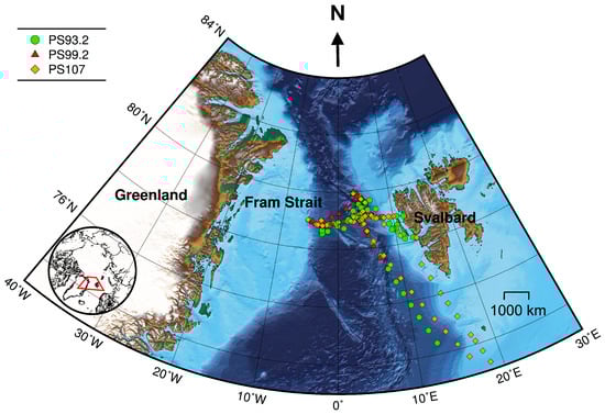
Figure 1.
Cruise tracks for PS93.2 (July–August 2015), PS99.2 (June–July 2016) and PS107 (July–August 2017). Symbols denote locations where both AC-S and HPLC data were collected. Bathymetric grid data are extracted from the International Bathymetric Chart of the Arctic Ocean Version 3.0 [62]. Lambert azimuthal equal-area projection was used for mapping.
The Fram Strait cruises PS93.2, PS99.2 and PS107 on R/V Polarstern collected a comprehensive in situ bio-optical data set and offer a unique opportunity for bio-optical modeling. In particular, underway spectrophotometry was applied during all three cruises. To obtain the information of individual phytoplankton pigments or pigment groups (e.g., PSC and PPC) from underway spectrophotometry, here, we compare and optimize the performances of two pigment retrieval approaches, Gaussian decomposition [22] and the matrix inversion technique [27,28], find the potential number and types of pigments that can be retrieved, and assess the applicability of the two approaches to the Fram Strait and its vicinity.
2. Data and Methods
2.1. Data Collection
Data were collected during three expeditions on R/V Polarstern: PS93.2 (July to August 2015), PS99.2 (June to July 2016) and PS107 (July to August 2017). These cruises have repeated survey design. Sampling sites were located in the Fram Strait and its vicinity, ranging from approximately latitudes 72 to 80N and longitudes 10W to 15E (Figure 1).
The underway and discrete pigment concentration measurements of the surface water were collected for each expedition. The average velocity of the ship while moving is ~10 knots (5.1 m s). Sampling methods and data analysis are detailed in Liu et al. [45]. Briefly, a 25-cm-pathlength AC-S spectrophotometer (spectral range: 400–740 nm, full width half maximum (FWHM): 10 nm, wavelength resolution: ~3.5 nm) was integrated into the shipboard flow-through system following the setup of Slade et al. [46]. Seawater was sampled at roughly 11 m below the sea surface from the ship’s keel using a membrane pump. The flow rate of seawater is 1–2 L min. The spectra were derived by subtracting the absorption coefficients of 0.2-μm filtered seawater from those of seawater materials measured by AC-S. Subsequently, they were corrected for temperature and salinity dependency of pure water absorption [63], scatter errors [64] and residual temperature effect [46]. Additionally, the effect of AC-S filter factors resulting in a smoothing of the measured spectra was corrected [22].
Discrete seawater samples were collected from the unfiltered AC-S outflow approximately every three hours. Seawater (1–3 L) was filtered with GF/F glass fiber filters (nominal pore size 0.7 μm) for HPLC phytoplankton pigment analysis (see Table 1 for the names and abbreviations of the pigments and pigment groups used in this study). Pigments were grouped following Hooker et al. [65]. Divinyl-chlorophyll-a and divinyl-chlorophyll-b were not found in our data set. For convenience, in the following context, the term “pigment” stands for either a specific type of pigment or a pigment group such as PSC and PPC. In addition, the spectral absorption coefficient of non-algal particles () in discrete water samples was measured for the determination of its spectral exponent. Seawater (0.2–1 L) was filtered to concentrate particulate materials on the GF/F filters. from discrete samples was determined using Quantitative Filter Technique [66,67,68]. Measurements for samples from PS93.2 were carried out on a dual-beam UV/VIS spectrophotometer (Cary 4000, Varian Inc., Palo Alto, CA, USA) (spectral range: 300–850 nm, FWHM: 2 nm, wavelength resolution: 1 nm) equipped with a 150 mm integrating sphere following Simis et al. [69], whereas filters collected during PS99.2 and PS107 were measured using a small portable integrating cavity absorption meter (spectral range: 300–850 nm, FWHM: 2 nm, wavelength resolution: 0.3 nm) [70], as detailed in Liu et al. [45]. was then obtained by measuring the sample filters bleached with 10% NaClO solution [69] following the same procedure as measurements. was approximated using an exponentially decaying function [71,72]:
where S is the spectral exponent of . Equation (1) was fit to for data between 380–620 nm excluding the 400–480 nm range (to eliminate residual chlorophyll-a absorption peak) using non-linear least squares method [72]. The median value of S for all three expeditions is 0.016 nm (standard deviation with respect to the median value is 0.006 nm), which was subsequently used in the decomposition of the AC-S derived to obtain (see Section 2.2.1).

Table 1.
Abbreviations of phytoplankton pigments and pigment groups analyzed in this study, and the minimum, maximum, mean and standard deviation of the pigment concentrations (mg m).
AC-S derived were averaged within the period of ten minutes before and after HPLC sampling time and were matched with HPLC pigments data. (400–700 nm, wavelength resolution: ~3.5 nm) was obtained by numerical decomposition (see Section 2.2.1). In total, 298 -pigments match-ups were obtained, which were subsequently used as the pigment retrieval data set. The link to the data used in this study is shared in the Supplementary Materials.
2.2. Retrieval of Phytoplankton Pigments
Figure 2 and Figure 3 illustrate the steps of applying Gaussian decomposition and the matrix inversion technique, respectively, to retrieve phytoplankton pigment concentrations, which are described in detail in the following subsections. The link to the codes for data processing is shared in the Supplementary Materials.
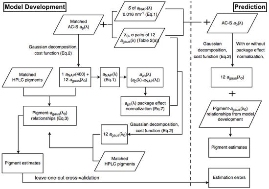
Figure 2.
Schematic overview of the steps of applying Gaussian decomposition for phytoplankton pigment retrieval.
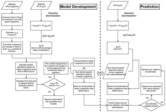
Figure 3.
Schematic overview of the steps of applying the matrix inversion technique for phytoplankton pigment retrieval.
2.2.1. Gaussian Decomposition
Following Chase et al. [22], AC-S derived was decomposed to twelve Gaussian functions and one exponential function expressed by Equation (1) in the range of 400–700 nm. Each Gaussian function represents the absorption by a certain phytoplankton pigment. The absorption by the water-soluble photosynthetic pigment phycoerythrin was also represented as a Gaussian function though its concentration could not be validated with HPLC. The peak location and width of each Gaussian function shown in Table 2 were defined with fixed values based on known pigment absorption shapes [73]. The decomposition is optimized by minimizing the cost function using a weighted least squares method [22]:
where denotes the ith Gaussian function, and is the standard deviation of the 20-min averaged matched spectra.
The amplitude of was derived by minimizing Equation (2) sample by sample and used to reconstruct for each sample according to Equation (1). was obtained by differencing and . The amplitude of each Gaussian function [m] was derived by minimizing Equation (2) and related to the concentration of the corresponding pigment measured by HPLC (c [mg m]) by fitting the following equation using Bisquare robust non-linear least squares method (data pairs with either or c being 0 were excluded) (Table 2):
For convenience, we denote the five pigments that can be retrieved using Gaussian decomposition (Table 2), i.e., TChl-a, TChl-b, Chl-c1/2, PSC and PPC as “Gauss-5 pigments”.
2.2.2. Matrix Inversion Technique
The spectra can be reconstructed as the linear combination of the absorption spectra of individual pigments that equal to the pigment-specific absorption coefficients () multiplied by pigment concentrations () [26], i.e., . When there is more than one sample in the observed collocated pigment concentrations and data set, the reconstruction model can be written in matrix multiplication form as:
where c is the observed pigment concentration (e.g., from HPLC), is the derived pigment-specific absorption coefficient, n is the number of samples, i is the sample index, m is the number of pigments measured in each sample, and j is the pigment index. The c and are known (the former from HPLC and the latter from spectrophotometry) while is unknown. To solve for , the elements of matrix , the inverse of matrix C is computed. Once this is done, the derived is used with the observed (l in Equation (5) is the number of wavelengths) to solve for the pigment concentrations ( in Equation (5)). Likewise, the computation of the inverse of matrix is necessary.
Hence, this is a two step approach. First, where HPLC is available, Equation (4) is used to obtain the pigment-specific absorption spectra. Once those are available, Equation (5) is used to derive pigment concentrations directly from (a step that does not require HPLC data). The SVD-NNLS approach proposed by Moisan et al. [27,28], i.e., solving Equation (4) with SVD least squares method on each wavelength and Equation (5) with NNLS method, was proved to give the best pigment estimates.
Singular Value Decomposition—Non-Negative Least Squares (SVD-NNLS)
The SVD-NNLS approach was adapted and tested using our data set. The matrix in Equation (4) (the concentrations of the pigments listed in Table 1) was inverted using SVD. The least-squares solution of the overdetermined Equation (4) (in this study ) is derived by , where is the Moore-Penrose pseudoinverse of matrix C computed by SVD (MATLAB function pinv). provides the specific absorption spectra of each pigment and is then used in Equation (5) to solve for pigment concentrations via NNLS (MATLAB function lsqnonneg), i.e., by inverting Equation (5) using least squares method with the constraint .
To ensure robust solutions of the overdetermined systems, matrix C in Equation (4) and matrix in Equation (5) should be constructed to avoid ill-conditioning, requiring that the columns and rows of matrix C have sufficient linear independence, and that the shapes of any two be sufficiently different from each other [36]. Here, we used the condition number () (MATLAB function cond) as a diagnostic for the degree of the well-conditioning of matrix C (a matrix with a high is ill-conditioned, and vice versa). In addition, a similarity index () [74,75] was used to represent the similarity between the absolute values of two specific spectra and (denoted as ). The is a number ranging from 0 (no similarity) to 1 (perfect similarity).
where is the norm of the vector (MATLAB function norm). To maximize the number of pigment types to be determined (m) while reducing the degree of the ill-conditioning, we tested all the possibilities of combining pigments composed of matrix C (number of combinations , 20 types of pigments measured in total) and examined and for all cases. For example, when m = 20, matrix C includes all the pigments listed in Table 1 excluding TChl-c, PSC and PPC (denoted as “Fram-20 pigments”) in 298 samples. When 1 < 20, matrix C includes the concentrations of m types of pigments and a summed contribution of other pigments included in the Fram-20 pigments. m was then determined as the biggest number with smaller than 60 and smaller than 0.9. For convenience, we denote the retrieval of these m pigments using SVD-NNLS as SVD-NNLS-m.
To compare with the results from Gaussian decomposition, the SVD-NNLS method was also applied to only retrieve Gauss-5 pigments (denoted as SVD-NNLS-5), i.e., matrix in Equation (4) only includes the concentrations of these five pigments and a summed contribution of other pigments.
The SVD derived specific absorption spectra are purely mathematical solutions. Therefore, they are expected to be different from those obtained through laboratory measurements performed on the extracted individual pigments in solution () [27]. For comparison, we tested the validity of NNLS in estimating pigment concentrations using from Bricaud et al. [73] in Equation (5). In this case, is available for 12 types of pigments (Divinyl-chlorophyll-a and divinyl-chlorophyll-b not considered), i.e., TChl-a, TChl-b, alloxanthin (Allo), But, Chl-c1/2, Diadino, Fuco, Hex, Peri, Zea, - and -Caro (denoted as “Bricaud-12 pigments”). The same criteria of and were used for all pigment combinations (number of combinations ). For each combination, the for the pigments which are missing in the Fram-20 pigments was solved using SVD (Equation (4), replaces ). We denote this case as Bricaud-SVD-NNLS, and the retrieval of m pigments as Bricaud-SVD-NNLS-m.
Non-Negative Least Squares—Non-Negative Least Squares (NNLS-NNLS)
Though SVD provides a powerful tool for matrix inversion, one concern is that the SVD derived specific absorption spectra can be negative, which are physically unsound and not intuitively understood. To cope with this issue, NNLS was used twice (denoted as NNLS-NNLS), i.e., to invert Equation (4) to solve for the non-negetive matrix , as well as to invert Equation (5) to derive the non-negative matrix . Similarly, NNLS-NNLS-5 was tested for comparison with the results from Gaussian decomposition and SVD-NNLS-5. Bricaud-NNLS-NNLS were also tested using the same way as Bricaud-SVD-NNLS with the exception that the for the missing pigments was solved using NNLS. The NNLS-NNLS approach was also performed by Moisan et al. [27,28]. The pigment estimation results from NNLS-NNLS are provided in Appendix A.
Sensitivity Analysis
The solution of matrix inversion can be sensitive to input errors depending on the degree of well-conditioning of the input matrices, which can affect the pigment estimation accuracy. To ensure the stability of the matrix inversion model and obtain reliable pigment estimation statistics, perturbations were introduced to the input data for 300 iterations, and the related parameters, i.e., , , and cross-validation statistics (see Section 2.2.4) were calculated as the median values of the 300 sets. Assuming an uncertainty of 15% for HPLC pigment data, matrix C was perturbed with random values within ±15% of the measurements. Matrix was also perturbed by adding the random values within (see Equation (2)) to the measurements. The results for three cases, i.e., with perturbed C, with perturbed and with both matrices perturbed were considered for both SVD-NNLS and NNLS-NNLS.
2.2.3. Normalization of by Pigment Package Effect
The pigment package effect index can be calculated as the ratio of the measured to the absorption coefficient of the same pigments which would be dispersed into solution [73,76]. To partially account for the package effect, Moisan et al. [27,28,34] normalized the measured by dividing it with and found improved capability of the matrix inversion technique in retrieving pigment concentrations. To test the performances of both Gaussian decomposition and the matrix inversion technique with the normalization strategy, was calculated, and was normalized following
where is TChl-a concentration (in mg m), 0.033 (in m mg) is the “unpackaged” Chl-a-specific absorption coefficient at 675 nm measured by Bricaud et al. [73], and the fraction is the inverse of . Note that chlorophyll-a, divinyl-chlorophyll-a, chlorophyll-b, divinyl-chlorophyll-b and Chl-c1/2 absorb light at 675 nm, e.g., [12,73]. For simplicity, we assume that is only contributed by TChl-a, not only because TChl-a contributes most to , but also due to the weaker dependence on pigment data for calculation. In theory, ranges from 0 (fully “packed”) to 1 (“unpackaged”). Due to uncertainties, samples with calculated greater than 1 are unavoidable in practise and included in the calculation of .
The was subsequently used to retrieve pigment concentrations via Gaussian decomposition, SVD-NNLS and NNLS-NNLS methods. Results were compared with those using . To avoid confusion, in the following context, unless otherwise stated, the results are based on .
2.2.4. Statistics
For the development of pigment retrieval models, all the match-up points were used as training data, allowing the models to best account for the biological variations in the data set. Statistics for applying the model to the training data include the slope and the intercept of Model-1 Bisquare robust linear regression, the determination coefficient (), the mean absolute error (MAE) and the median absolute percentage error (MPE). The equations for the statistical metrics are given below:
where n is the number of samples, is the concentration of the jth pigment in the ith sample measured by HPLC, and is the estimated pigment concentration. Considering phytoplankton pigments are approximately log-normally distributed in the ocean, the slope, intercept and were computed in log10 space. Additionally, MAE is also calculated using log10(). To avoid confusion, in the following context, unless otherwise stated, MAE values are calculated using .
For model evaluation, leave-one-out cross-validation was performed (MATLAB function crossvalind) to estimate likely performance of each model on out-of-sample data. The pigment retrieval data set with N data points was split into two partitions: one partition is the testing set with one data point, and the other partition is the training set with the union of the other data points. Statistics were iteratively calculated N times, using a different data point as the testing set each time. The model prediction errors for out-of-sample data were defined as the average values of the statistics (mean value for MAE and median value for MPE, respectively) for the N sets. Cross-validation is an effective way of estimating model test errors when the number of data available is relatively small [18,77]. Compared to the random train/test split method and k-fold cross-validation, leave-one-out cross-validation has the advantage that the training set highly resembles the whole data set (the former has only one data point less than the latter), thus avoids the bias introduced to the estimation of the test errors due to less training data than data available.
For clarity, statistics (errors) obtained from running the trained model back on the training data are denoted as “training statistics (errors)”, while those obtained when applying the trained model to the test data are called “test (or estimation or prediction) statistics (errors)”.
3. Results
3.1. Characteristics of the Pigment Retrieval Data Set
The magnitudes of and vary in the range of 0.007–0.258 m (median: 0.043 m) and 0.001–0.086 m (median: 0.013 m), respectively. Overall, varies as a power function of TChl-a concentration (Bisquare robust regression): ( = 0.82, MAE = 0.01 m). This relationship is close to the one derived by Bricaud et al. [71] for Case-1 waters (Figure 4a). TChl-a can also be related to via the cruise-specific power functions (Bisquare robust regression): ( = 0.96, MAE = 0.12 mg m) (PS93.2), ( = 0.96, MAE = 0.14 mg m) (PS99.2), and ( = 0.95, MAE = 0.17 mg m) (PS107).
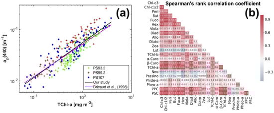
Figure 4.
(a) Variations of the AC-S derived as a power function of TChl-a concentration; (b) the Spearmans rank correlation coefficients between the concentrations of phytoplankton pigments in our data set (linear color bar scale).
The composition and data range of pigments (minimum, maximum, mean and standard deviation) are shown in Table 1. TChl-a concentration spans the range 0.06–3.87 mg m. Only TChl-a, TChl-c, Fuco, Hex and PSC have a mean concentration greater than 0.2 mg m. Other than that, the pigments with mean concentrations greater than 0.05 mg m are Chl-c1/2, Diadino, TChl-b, and PPC. Large standard deviations were observed within individual pigments, and the ratios of standard deviation to mean value are in the range of 0.58–4.35. The correlation between the concentrations of phytoplankton pigments was represented by the Spearmans rank correlation coefficient (Spearman’s ) (Figure 4b). High level of the correlation (e.g., Spearman’s > 0.7 or <−0.7) is a concern as it can cause the ill-conditioning of Equation (4), influencing the accuracy of pigment estimation using the matrix inversion technique.
3.2. Gaussian Decomposition
Strong correlations were found between the Gaussian function amplitudes and the corresponding pigment concentrations () (Table 2 (a)). Among all the Gaussian functions representing TChl-a absorption, the amplitude at 434 nm has the strongest relationship to TChl-a concentration ( = 0.87, MAE = 0.21 mg m), closely followed by that at 675 nm. is much better correlated with Chl-c1/2 than , while provides slightly better correlation with TChl-b than . That the for TChl-b and PPC is smaller than 0.6 is likely due to the reduced dynamic range of TChl-b and PPC compared to TChl-a, Chl-c1/2 and PSC (Table 1). Considering the relationships for PSC and PPC as well as the strongest correlations for TChl-a, TChl-b and Chl-c1/2, the MPE ranges from 20.7% to 33.4%. The training errors for the five pigments increase in the order of: TChl-a, TChl-b, PPC, Chl-c1/2 and PSC. The strongest correlations for all five pigments are shown in Figure 5a,c,e,g,i. For comparison, TChl-a is also plotted against in Figure 5k.
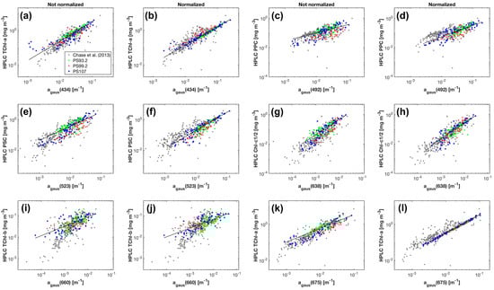
Figure 5.
Concentrations of phytoplankton pigments measured by HPLC versus the magnitudes of the corresponding Gaussian functions obtained from the Gaussian decomposition of both (a,c,e,g,i) and (b,d,f,h,j,l). The results of Chase et al. [22] are based on .
As a result of the above, , , , and were used to predict the concentrations of TChl-a, TChl-b, Chl-c1/2, PSC and PPC, respectively. Statistics based on leave-one-out cross-validation (Table 2 (a)) show that overall, all five pigments were reasonably well retrieved (MPE 20.8–34.0%). TChl-a and TChl-b have the least and the second least prediction errors, respectively, while PSC is most poorly estimated.
When using , the performance of the Gaussian decomposition significantly improved. Strong contrast was observed in the relationships between the Gaussian function amplitudes and pigment concentrations before and after applying the package effect normalization according to Equation (7) (Figure 5, Table 2 (b)). All statistical parameters for the eleven relationships between Gaussian absorption and pigment concentrations are improved (Table 2 (b)). The for to TChl-a correlation is 0.96 (0.87 before the normalization) and the regression coefficient B (Equation (3)) is close to one. Similarly, the for to Chl-c1/2 correlation is 0.91 (0.81 before the normalization) and the regression coefficient B (Equation (3)) is also close to one. The relationships for PSC and PPC also improved in terms of increased and decreased MAE and MPE for both pigments, and of a much closer shift of B (Equation (3)) to one for PPC. In contrast, the relationship for TChl-b is least affected by the package effect normalization of , with still increased , but only slightly decreased MAE and MPE, and a relatively large deviation of B (Equation (3)) to the unity (0.35–0.60 for both 470 nm and 660 nm regardless of the normalization). Cross-validation results (Table 2 (b)) further confirm the improved performance of Gaussian decompostion in estimating TChl-b, Chlc1/2, PPC and PSC after taking the package effect into account (MPE 29.3–34.0% before the normalization and 20.5–27.4% afterwards). The pigment with the lowest estimated accuracy is now Chl-c1/2, but still with an improved accuracy following normalization. Similarly, TChl-b retrievals have slightly reduced MAE and MPE than those before the normalization.
3.3. Matrix Inversion Technique
3.3.1. The Number of Pigment Types to Be Estimated
To apply the matrix inversion technique to estimate phytoplankton pigments, a key issue is to determine the number of pigments m included in matrix C in Equation (4). Table 3 summarizes the final selections of m that fulfilled the criteria mentioned in Section 2.2.2 and the corresponding and for all cases of the matrix inversion technique. The and maximum values of did not significantly change after data perturbations were introduced, regardless of the application of the package effect normalization.
As shown in Figure 6, the minimum values of for all pigment combinations increase with increasing m, indicating that the larger the number of pigment types to be estimated, the more sensitive the matrix inversion is to input errors. The largest value of m is nine and six for all combinations of Fram-20 and Bricaud-12 pigments, respectively, with the minimum value of smaller than the threshold 60. When composed of Gauss-5 pigments, matrix C has a of 47.8.
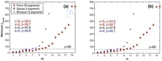
Figure 6.
Variations in the minimum values of the condition number () of matrix C in Equation (4) with different pigment combination (m pigment types to be estimated): (a) pigment data unperturbed; (b) pigment data perturbed.
Based on the results fulfilling the criterion, when is derived by SVD, the criterion allowed m to reach nine out of the Fram-20 pigments, and was satisfied by the Gauss-5 pigments. However, m for the NNLS-NNLS method decreased to six for of the Fram-20 pigments when package effect normalization was not performed, because the NNLS algorithm set some of the derived in the pigment combinations (m > 6) to zero to avoid negative values [30]. When the package effect normalization was applied, the number of pigment combinations valid for calculation increased to nine, possibly because this normalization increases the inner differences of the set of the derived . However, the maximum value exceeded 0.9 for Gauss-5 pigments. Therefore, NNLS-NNLS-5 method based on was not considered in the estimation of pigments. As for the Bricaud-12 pigments, the choice of SVD and NNLS influences the derived specific absorption of the missing pigments, as indicated by the different values. In this case, m reaches four. The specific pigments to be inverted for all cases are shown in Table 4 and Table 5 and Table A1.
3.3.2. SVD-NNLS
The pigment-specific absorption coefficients obtained from SVD-NNLS-9, SVD-NNLS-5 and Bricaud-SVD-NNLS-4 without input data perturbations are displayed in Figure 7. Each SVD derived specific spectra varies smoothly across the full bands and sufficiently differs from each other ( < 0.9). Negative coefficients are permissible because these are mathematical constructs. Pigment concentration estimates were then solved via NNLS and compared to HPLC pigment concentrations. Training statistics (Table 4) and the scatter plots (Figure 8) show that the estimated and the corresponding measured pigments were correlated ( > 0.30) except for Pheo-a (SVD-NNLS-9), TChl-b (SVD-NNLS-5) and Hex (Bricaud-SVD-NNLS-4). For SVD-NNLS-9, the training errors for all pigments except for Peri and Pheo-a were reduced by the package effect normalization (Table 4 (a)). In contrast, this normalization increased training errors when using Bricaud-SVD-NNLS-4 (Table 4 (c)). For SVD-NNLS-5, all Gauss-5 pigments except for PPC were observed to have smaller training errors with this normalization (Table 4 (b)).
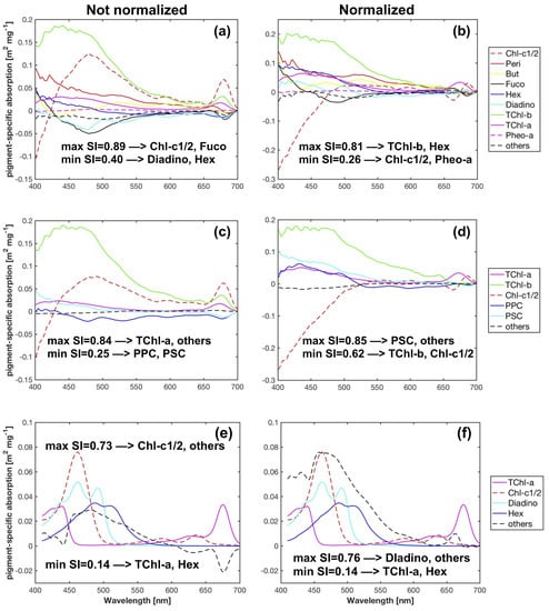
Figure 7.
Pigment-specific absorption spectra obtained from SVD-NNLS-9 (a,b), SVD-NNLS-5 (c,d) and Bricaud-SVD-NNLS-4 (e,f) without data perturbations, respectively. Cases with and without package effect normalization were compared.
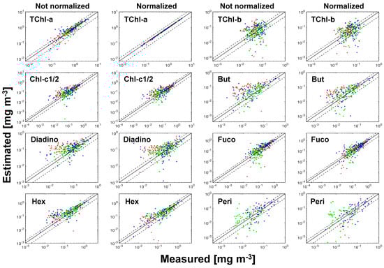
Figure 8.
Scatter plots of SVD-NNLS-9 estimated pigment concentrations versus measured pigment concentrations for unperturbed training data set. The symbols of green circles, red crosses and blue stars represent the data from the cruises PS93.2, PS99.2 and PS107, respectively. Dash lines denote the 50% error lines, and solid lines are one-to-one lines.
To obtain robust pigment estimation statistics and evaluate the influences of the package effect normalization on them, data perturbations and cross-validation were combined to generate the test errors (Table 5). The SVD-NNLS-9 method (Table 5 (a)) exhibited stable prediction accuracy (MPE 16–65%) for six types of pigments, i.e., TChl-a, TChl-b, Chlc-1/2, Diadino, Fuco and Hex, in which MPE varied less than 10% and MAE less than a factor of 1.2 with input data perturbations. TChl-a had the least prediction error (MAE 0.17–0.22 mg m, MPE 16–22%); Fuco, Hex and Chl-c1/2 shared the second best estimation (MPE 35–45%); Diadino was least accurately estimated (MAE 0.07–0.08 mg m, MPE 61–65%), and TChl-b showed a slightly smaller MPE of 53–60% (MAE 0.03–0.04 mg m). Though included in the calculation, But, Peri and Pheo-a exhibited relatively inconsistent prediction errors with the three cases of data perturbations, likely because of their relatively low concentrations (Table 1) and infrequent occurrence in the data set. When considering the package effect normalization, however, all nine pigments except for Pheo-a achieved stable prediction statistics (MPE 36–76%) with the different cases of data perturbations (MPE varied less than 13% and MAE less than a factor of 1.3, Table 5 (a)). The normalization obtained comparable prediction errors as those without normalization for TChl-b, Diadino and Hex, 8% higher of MPE for Chlc-1/2 and Fuco, and additional estimations of But (MPE 67–70%) and Peri (MPE 68–75%).
For SVD-NNLS-5 (Table 5 (b)), all five pigments were stably retrieved (MPE 17–73%). TChl-a and PSC had the lowest prediction errors (MPE 17–23% and 35–43%, respectively), whereas TChl-b was most poorly estimated (MPE 58–73%). Chl-c1/2 and PPC exhibited similar retrieval accuracy (MPE 48–69%). In comparison, the estimation errors with the application of the package effect normalization did not significantly change for TChl-b, Chlc-1/2 and PSC, and slightly increased for PPC.
The Bricaud-SVD-NNLS-4 method provided stable retrieval statistics for all four pigments (Table 5 (c)). The prediction errors increased in the order of TChl-a (MPE 25–27%), Chlc-1/2 (MPE 32–34%), Diadino (MPE 77–80%) and Hex (MPE 82–84%). When using , the overall performance of this method was significantly hindered for Diadino and Hex (MPE increased ~40%) and slightly affected Chl-c1/2 (MPE increased ~10%).
3.3.3. Intercomparison between SVD-NNLS Applications
SVD-NNLS-9 and SVD-NNLS-5 showed similar capabilities in retrieving TChl-a, and both methods outperformed Bricaud-SVD-NNLS-4 (Table 5). SVD-NNLS-9 surpassed SVD-NNLS-5 in retrieving TChl-b and Bricaud-SVD-NNLS-4 in the retrieval of Diadino and Hex, respectively. For Chl-c1/2, Bricaud-SVD-NNLS-4 performed the best and SVD-NNLS-5 the worst. Considering the overall pigment retrieval accuracy and the number of pigment types possible to retrieve, SVD-NNLS-9 performed best among the three SVD-NNLS methods.
3.3.4. Feasibility of SVD-NNLS-9 for Multispectral
The performance of the matrix inversion technique is sensitive to the number of wavebands and their locations on the spectrum [27,33]. To test the feasibility of this technique using multispectral , SVD-NNLS-9 was performed with at ten MODIS bands, i.e., 412, 443, 469, 488, 531, 547, 555, 645, 667 and 678 nm. In this case, only four types of pigments, i.e., TChl-a, TChl-b, Chlc-1/2 and Hex, were retrieved with stable and acceptable estimation statistics (Table 6) both with and without package effect normalization. The estimation errors of TChl-a and TChl-b slightly increased by 4 to 14% using multispectral , while for Chlc-1/2 and Hex, the MPE were approximately 30% and 20% higher than those with hyperspectral , respectively.
Table 6.
Statistics of phytoplankton pigment retrieval using SVD-NNLS-9 with at ten MODIS bands based on leave-one-out cross-validation. MAE is in mg m (values outside the parentheses were calculated with linear-scale values, while inside the parentheses with log10-scale values) and MPE in %. “Perturb 1, 2 and 3” represent the input data with perturbations of pigment concentrations solely, solely and both, respectively.
3.4. Gaussian Decomposition versus SVD-NNLS
Considering both MAE and MPE, the Gaussian decomposition method revealed comparable capability in estimating TChl-a compared to SVD-NNLS-9 and SVD-NNLS-5 (Table 2 and Table 5 (a,b)). However, it outperformed SVD-NNLS-5 in retrieving TChl-b (MPE ~ 40% lower), Chl-c1/2 (MPE ~ 35% lower), PSC (MPE ~ 8% lower) and PPC (MPE ~ 30% lower) and surpassed SVD-NNLS-9 in predicting TChl-b (MPE ~ 30% lower) and Chl-c1/2 (MPE ~ 12% lower). When the package effect normalization was applied, the results from Gaussian decomposition further improved the estimation of the Gauss-5 pigments (TChl-a excluded).
4. Discussion
The study of phytoplankton dynamics in relation to a changing climate requires access to high resolution phytoplankton pigment information in space and time. Unlike data obtained from HPLC analysis of discrete water samples, underway spectrophotometry is capable of providing nearly continuous in situ data records of spectral particulate absorption as well as phytoplankton absorption. The latter is dependent on the concentrations and composition of phytolankton pigments. Therefore, algorithms that link hyperspectral obtained from underway spectrophotometry to the concentrations of various phytoplankton pigments provide pigment information with high spatial resolution (~300 m for one minute binned-averaged spectra when the ship is moving at ~10 knots). This pigment information can support the evaluation of ocean color algorithms and coupled hydrodynamic-biological modelling. With the advancement of hyperspectral radiometers, these algorithms have great potential to be incorporated into the inversion of satellite ocean color measurements for the synoptic detection of phytoplankton pigments and thus the monitoring of phytoplankton spatial and temporal dynamics.
Gaussian decomposition is an effective pigment retrieval algorithm that dates back to 1990s [11] and was recently modified for more extended applications, e.g., [22,23,24,25]. At the time this manuscript is drafted, it is the only method that has been applied to underway spectrophotometry data and successfully retrieved the concentrations of various pigments [22]. Compared with Gaussian decomposition and other methods from previous studies, e.g., [14,15,19,26] that are incapable of resolving PPC and PSC, the matrix inversion technique is capable of estimating these and various marker pigments indicative of phytoplankton composition [27,28,34]. Both Gaussian decomposition and the matrix inversion technique rely on the physical links between phytoplankton pigments and their distinct light absorption properties, while other methods’ (e.g., principle component analysis) output is often physically uninterpretable.
To assess the utility of the two methods and improve their performances in our study area, we improved the Gaussian decomposition algorithm from Chase et al. [22] by considering pigment package effect and reconsidered the matrix inversion technique from Moisan et al. [27] by taking into account matrix conditioning. In the following discussion, we compare the results from this study to those from the literature, highlight the improvements we have made, and show applications to underway absorption data.
4.1. Gaussian Decomposition
Our -pigment data falls into the range of the global data set from Tara expeditions [22] and has a large portion of overlap with the global data (Figure 5, Table 7) except for TChl-b (Figure 5i), likely due to the lack of low TChl-b concentrations in this study. Furthermore, our -pigment data shows less scatter (Figure 5a,c,e,g,i,k), and the estimation errors for all Gauss-5 pigments are lower than those of the Tara data set (MPE 7.5–20% lower). This is probably because of a higher level of variability in pigment package effect of the global data set than that in the Fram Strait, as indicated by the greater quartile coefficient of dispersion of the pigment-specific absorption coefficient (, defined as the ratio of to the corresponding pigment concentration) for the global data set (Table 7). In addition, it could also be due to the errors introduced by the extent of the Tara expeditions study (2.5 years) and resulting increased potential for methodological variability, while only four people were involved in discrete sampling in the current study.
Table 7.
The range of values, median and quartile coefficient of dispersion (CD) for the Gaussian decomposition derived pigment-specific absorption coefficient at the corresponding wavelength (in m mg).
After applying the package effect normalization, as expected, almost all the -TChl-a data points fall on the regression line (Figure 5l, Table 2), i.e., no additional package effect was found at , suggesting the successful simplification of calculation using only TChl-a concentration. Both the for to TChl-a correlation and the regression coefficient B (Equation (3)) are close to one, indicating that the variations in the magnitude of account for a large proportion of the variations in the package effect due to TChl-a at 434 nm. Similar improvements have been observed for Chl-c1/2, PSC, PPC and to a less extent, TChl-b, which implicates the covariation between the package effect of these pigments at the corresponding wavelengths and that of TChl-a. This is also proved by the reduced data dispersion of except for TChl-b (Table 7) and the strong power law relationships ( 0.39–0.87) between , , , , and , respectively. The package effect of a specific pigment is a function of the concentration of this pigment as well as phytoplankton cell size [76]. The strong correlations between TChl-a concentration and the concentrations of Chl-c1/2 (Spearman’s = 0.9), PSC (Spearman’s = 1.0), PPC (Spearman’s = 0.8), and of TChl-b (Spearman’s = 0.7) (Figure 4b) explain the covariation of the package effect by the pigments.
In essence, the Gaussian decomposition method takes advantage of the absorption-pigment concentration correlation. The shape and magnitude of is controlled by phytoplankton pigment composition and the level of the pigment package effect. When applying Gaussian decomposition, the absorption of individual pigments were separated and related to corresponding pigment concentrations. Therefore, the effects of pigment composition and package were separated, and the observed variations in absorption-pigment concentration correlation are mainly attributed to the package effect. The covarying absorption by more than one pigment that failed to be separated by this method is also a reason for these variations. Though simplified, the package effect is for the first time taken into account during Gaussian decomposition of and improved the pigment estimation accuracy. It provides new insight into increasing pigment retrieval accuracy via the combined use of concurrent and TChl-a concentration either obtained from field instrumental measurements/estimates or satellite data. To test the applicability of this normalization to underway spectrophotometry data when HPLC TChl-a data is not available, TChl-a was firstly calculated from the AC-S derived via the cruise-specific power functions (see Section 3.1). In this case, the improvement was also found with the normalization (Table 8). However, when TChl-a was derived either from using the power law relationship described in Section 3.1 or the global relationship from Bricaud et al. [71], no improvement was observed (results not shown), possibly because of the more accurate TChl-a derived by the cruise-specific relationships. Therefore, the improved performance with this normalization relies on the accurate measurement or derivation of TChl-a data. An improved method for calculating pigment package effect is needed so that the calculation is independent of HPLC TChl-a data. Lin et al. [78] developed an optimization approach in estimating from in the range of 650–700 nm based on pigment package effect theory. We tested this method and found that the calculated did not improve retrievals (results not shown ). In summary, better results can be expected by further deciphering the influence of pigment package effect on the absorption-pigment concentration relationship.
Table 8.
Statistics of phytoplankton pigments retrieval using Gaussian decomposition with package effect normalization based on leave-one-out cross-validation. Package effect normalization was performed with in Equation (7) calculated using cruise-specific (AC-S)-TChl-a (HPLC) relationships (see Section 3.1). MAE values outside the parentheses were calculated with linear-scale values, while inside the parentheses with log10-scale values.
4.2. Matrix Inversion Technique
Compared to the seemingly physically interpretable NNLS derived and the measured from extracted pigments in solution, the usage of the SVD derived provided the most robust pigment estimates, though non-negative specific absorption cannot be guaranteed. This is consistent with the previous study from Moisan et al. [27]. It is worth noting that neither of the two types of nor the measured are representative of the real in vivo "unpacked" pigment-specific absorption coefficient used in the reconstruction model. The former are pure mathematical optimization solutions based on least squares or constrained least squares minimization.
The different estimation errors of SVD-NNLS-9 and SVD-NNLS-5 for TChl-b and Chlc-1/2 (Table 5 (a,b)) suggest the performance of SVD-NNLS in estimating pigments differs with the different way of grouping pigments for matrix C (Equation (4)). The estimation accuracy of a specific pigment using SVD-NNLS-9 and SVD-NNLS-5 increases with the increase of the amount of the pigment in the samples, which was also observed by Moisan et al. [27]. The similar estimation statistics of all three SVD-NNLS methods for TChl-a (Table 5) is probably because TChl-a is the main pigment of phytoplankton and contributes the most to .
Moisan et al. [27] found that with the package effect normalization, the SVD-NNLS method yielded much better predictions of pigments. In this study, when considering the training accuracy of SVD-NNLS-9 and SVD-NNLS-5 (Table 4 (a,b)), most of the pigments showed improved MAE and MPE with this normalization. However, the cross-validation results calculated by taking into account the data perturbations (Table 5 (a,b)) showed randomly improved, reduced, or similar pigment prediction errors after the application of the normalization. The reason for this inconsistency is probably due to the fact that both Moisan et al. [27] and the training statistics in this study did not take into account the sensitivity of matrix inversion to input errors. Moisan et al. [27] also pointed out that the inverse model solutions are sensitive to the level of errors in the measured . The inconsistency between the results of the training (Table 4) and test errors (Table 5) confirms this sensitivity and that in this case, the training statistics are not appropriate for use to indicate pigment estimation errors. The results from cross-validation with data perturbations, on the other hand, encompassed the training statistics as their one special case and effectively reduced the sensitivity of the SVD-NNLS method to provide robust and stable pigment estimation statistics. Nevertheless, when performing package effect normalization on SVD-NNLS-9, two more pigments with lower concentrations also obtained robust statistics, possibly due to the enhancement of the differences between of different pigments.
The sensitivity of the matrix inversion technique comes from the ill-conditioning of the linear systems (Equations (4) and (5)), which originates from the multicollinearity of phytoplankton pigments. In natural water samples, the multicollinearity of phytoplankton pigments (Figure 4b) are physiologically unavoidable. In other words, the ill-conditioning of Equations (4) and (5) is not completely avoidable. To reduce the degree of the ill-conditioning, the choice of the pigments included in matrix C (Equation (4)) is crucial. Our proposed and criteria to determine which pigments should be inverted for is empirically based on the understanding of the characteristics of the input data and many trials. The thresholds of and may change from case to case. The sensitivity analysis based on data perturbations (Table 3) shows the relative stable values of and . This is consistent with the singular value perturbation theorems [79], i.e., the singular values of a matrix are very stable with respect to changes in the elements of the matrix, because the is by definition the ratio of the largest to smallest singular values of a matrix. In contrast, though aware of the multicollinearity issue, Moisan et al. [27] did not pre-select the pigments to be determined. Instead, all types of pigments available from HPLC were included in the inverse modelling, which was also tested by this study (results not shown) and can lead to reduction of the pigment retrieval accuracy.
4.3. Applications
With the particulate absorption data collected by underway AC-S flow-through system, phytoplankton pigment concentrations along the cruise tracks are retrieved. Figure 9 shows an example of the underway Fuco and Hex estimated by SVD-NNLS-9. Fuco and Hex are dominant in diatoms and prymnesiophytes, respectively, which are the two common phytoplankton groups in the Fram Strait, e.g., [56]. However, we have to bear in mind that differentiating phytoplankton groups by marker pigments can be problematic, as there is substantial variability in pigment concentrations as a function of physiological responses to the environmental conditions. More importantly, a given marker pigment can be present in several phytoplankton groups (e.g., Fuco in diatoms and prymnesiophytes; more details in Wright and Jeffrey [80]). Data from the year 2015 indicates a co-prosperity of diatoms and prymnesiophytes. Overall, the concentrations of Fuco are relatively higher than those of Hex, which possibly reflects an overall higher biomass of diatoms (Figure 9a). In the year 2016, while this co-prosperity continued, the Hex concentrations exceeded the concentrations of Fuco in the western part of our study area (2 July 2016) (Figure 9b). In contrast, the year 2017 experienced an overall higher concentrations of Hex than Fuco (Figure 9c). These results are consistent with previous observations of the shift of phytoplankton assemblages from diatoms to Phaeocystis spp.(a type of prymnesiophyte) during the summer months in the Fram Strait [56,58,59]. In the future, access to similar high resolution phytoplankton pigment data verified by microscopic and flow cytometric techniques could support the studies on biogeophysical coupling in the Fram Strait and further enhance our understanding in the responses of phytoplankton community composition and physiology to climate change.
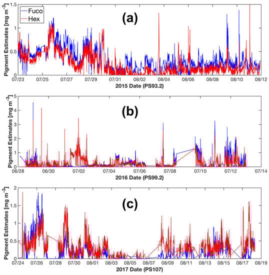
Figure 9.
SVD-NNLS-9 estimated Fuco and Hex concentrations from underway spectrophotometry during the cruise periods of PS93.2 (a), PS99.2 (b) and PS107 (c).
5. Conclusions
We demonstrated the retrieval of high spatially resolved phytoplankton pigment concentrations in the Fram Strait and its vicinity from underway hyperspectral (400–700 nm, ~3.5 nm wavelength resolution) by the application of Gaussian decomposition [22] and the matrix inversion technique [27]. Gaussian decomposition enables robust predictions of Gauss-5 pigments (MPE 21–34%). Improved retrieval accuracy was obtained by normalizing the spectra with the pigment package effect factor at 675 nm. For the matrix inversion technique, although SVD cannot guarantee the derivation of non-negative pigment-specific absorption spectra, it generates more accurate pigment estimates compared to the NNLS derived spectra or the measured spectra from pigments in solution. To minimize the effect of the ill-conditioned matrices on pigment retrieval accuracy, we propose an innovative approach in selecting the pigments to be determined based on the combined use of data perturbations and leave-one-out cross-validation to generate robust pigment estimation statistics. Considering the overall pigment retrieval accuracy, SVD-NNLS-9 performed best among the three SVD-NNLS methods. The SVD-NNLS-9 method enables the robust estimations of six pigments (MPE 16-65%), i.e., TChl-a, TChl-b, Chl-c1/2, Diadino, Fuco and Hex, and two more being less accuraely estimated (MPE 67–76%), i.e., But and Peri, with the application of the package effect normalization. Gaussian decomposition outperforms SVD-NNLS-5 in retrieving the TChl-b, Chl-c1/2, PPC and PSC, while both methods show similar capability in estimating TChl-a.
The matrix inversion technique has the advantage of retrieving the concentrations of several specific carotenoids, which is currently not accomplished by Gaussian decomposition, derivative analysis [13], partial least squares regression [14], and multiple linear regression [15]. However, its performance is sensitive to input errors when the input matrix is to some extent ill-conditioned. Therefore, sensitivity analysis such as the one based on data perturbations used in our study is always needed when assessing the performance of the matrix inversion technique in retrieving phytoplankton pigments or pigment related parameters. Future studies using methods such as principle component analysis and artificial neural network may show promise to obtain not only chlorophylls but also different types of carotenoids in our study area.
In addition to the number of pigments, the number of spectral bands used for pigment retrieval also significantly influence the performance of the matrix inversion technique. Compared with the results using hyperspectral , the number of pigments able to be retrieved by SVD-NNLS-9 was reduced to four, i.e., TChl-a, TChl-b, Chl-c1/2 and Hex, with increased estimation errors, especially for Chl-c1/2 and Hex, when using multispectral (at ten MODIS bands). This suggests the advantage of using hyperspectral data for increasing the accuracy of phytoplankton pigment retrievals. It follows that inverted from hyperspectral remote sensing reflectance measured by in situ or satellite radiometry has a greater potential for the application of Gaussian decomposition and the matrix inversion technique than multispectral radiometric measurements.
To apply Gaussian decomposition or the matrix inversion technique to a study area, prior knowledge of concurrent AC-S derived and HPLC pigment concentrations in this region is necessary to derive either the regional -pigment concentration relationship or the regional pigment-specific absorption spectra. With this knowledge, we apply both approaches to underway AC-S measurements in times when no HPLC data is available. Given that proxy-relation may change in the future, it is imperative to always collect some HPLC data to validate that derived relations or coefficients are still consistent.
The application of the two methods to our data obtain in three Fram Strait expeditions enables the derivation of pigment data sets along the cruise tracks. Future work could build upon these results, by deriving phytoplankton functional types based on retrieved marker pigments from hyperspectral phytoplankton absorption as well as hyperspectral remote sensing reflectance data. Such a high resolution data set will strengthen the study of phytoplankton dynamics in responses to environmental variables in the context of climate change.
Supplementary Materials
The quality controlled particulate absorption data from underway AC-S flow-through system, the HPLC phytoplankton pigments from discrete samples, and the estimated pigment concentrations along cruise tracks mentioned in this paper are available on PANGAE: https://doi.pangaea.de/10.1594/PANGAEA.894875. The MATLAB codes for data processing are available online at https://github.com/phytooptics.
Author Contributions
A.B. and Y.L. conceived and designed the experiments; Y.L. collected HPLC pigments data from the expeditions PS99.2 and PS107, and processed AC-S absorption data from all three expeditions; Y.L. led the data analysis and all coauthors assisted in it; E.B., A.C., A.B., H.X., X.Z. and R.R. helped with the interpretation of the data; E.B. and A.C. contributed the software of Gaussian decomposition and its application to this study; Y.P. contributed to programming and data visualization; Y.L. drafted the manuscript and all coauthors provided substantial comments and suggestions to improve it.
Funding
This research was funded by the Helmholtz Association Infrastructure Programme FRontiers in Arctic marine Monitoring (FRAM), the Deutsche Forschungsgemeinschaft (DFG, German Research Foundation)—Projektnummer 268020496—TRR 172, within the Transregional Collaborative Research Center “ArctiC Amplification: Climate Relevant Atmospheric and SurfaCe Processes, and Feedback Mechanisms (AC)” project C03, and NASA Ocean biology and biogeochemistry grant NNX15AC08G. Y.L.’s fellowship is funded by the China Scholarship Council. Y.L.’s travel grants were funded by POLMAR Helmholtz Graduate School for Polar and Marine Research of the Alfred Wegener Institute.
Acknowledgments
We thank the captains, crew and scientists, espcially the chief scientists—Thomas Soltwedel and Ingo Schewe for supporting our work on R/V Polarstern during the expeditions PS93.2, PS99.2 and PS107. We thank Sonja Wiegmann for the HPLC analysis of pigments from the filtered water samples. We thank Sonja Wiegmann, Marta Ramírez-Pérez and Sebastian Hellmann for their help in collecting samples and runing the AC-S instrument during the expeditions. We acknowledge the use of Generic Mapping Tool (GMT) for geographical mapping. Thanks to Junfang Lin for the discussions of optical theories of the pigment package effect. Thanks to Annick Bricaud for providing pigment-specific absorption coefficients data used in Bricaud et al. [73]. Thanks to John Moisan for helping apply SVD-NNLS method to our data set. Thanks to Borut Umer and Karlis Mikelsons for the discussions of SVD related issues. Thanks to Jan Streffing and Nils Haëntjens for helping program using MATLAB. Thanks to Florian Riefstahl for helping with data visualization. Thanks to three anonymous reviewers whose comments significantly improved the manuscript.
Conflicts of Interest
The authors declare no conflict of interest.
Abbreviations
The following mathematical parameters are used in this manuscript:
| Symbol | Description |
| Gaussian absorption coefficient (Equation (2)) | |
| spectral absorption coefficient by non-algal particles | |
| spectral particulate absorption coefficient | |
| spectral phytoplankton absorption coefficient | |
| pigment package effect normalized (Equation (7)) | |
| A | matrix of (Equations (4) and (5)) |
| real or measured pigment-specific absorption coefficient | |
| SVD or NNLS derived pigment-specific absorption coefficient (Equations (4) and (5)) | |
| absolute values of (Equation (6)) | |
| norm of (Equation (6)) | |
| matrix of (Equations (4) and (5)) | |
| A | regression coefficient of pigment concentration- power relationship (Equation (3)) |
| B | regression coefficient (power) of pigment concentration- power relationship |
| (Equation (3)) | |
| c | HPLC derived pigment concentration |
| C | matrix of c (Equation (4)) |
| C | Moore–Penrose pseudoinverse of matrix C |
| HPLC derived TChl-a concentration | |
| estimated pigment concentration | |
| matrix of (Equation (5)) | |
| CD | quartile coefficient of dispersion |
| m | number of pigment types |
| MAE | mean absolute error (Equation (8)) |
| MPE | median absolute percentage error (Equation (9)) |
| n | number of samples |
| condition number of matrix C | |
| determination coefficient | |
| S | spectral exponent of (Equation (1)) |
| similarity index between two (Equation (6)) | |
| Spearman’s | Spearmans rank correlation coefficient |
| pigment package effect index | |
| peak wavelength of a Gaussian function | |
| width of a Gaussian function | |
| standard deviation of the 20-minute averaged matched AC-S spectra (Equation (2)) | |
| cost function of Gaussian decomposition (Equation (2)) |
Appendix A. Cross-Validation Results of NNLS-NNLS
As shown in Table 5 and Table A1, overall, pigment estimation errors from NNLS-NNLS were larger than the corresponding SVD-NNLS for all pigments excepte for TChl-a. The NNLS-NNLS-6 method exhibited robust predictions for TChl-a, Fuco and Hex (MPE 21–65%). With the package effect normalization, three more pigments, i.e., TChl-b, Chl-c1/2 and But were reasonably estimated (55–82%).
Table A1.
Statistics of phytoplankton pigment retrieval using NNLS-NNLS based on leave-one-out cross-validation. MAE is in mg m (values outside the parentheses were calculated with linear-scale values, while inside the parentheses with log10-scale values) and MPE in %. “Perturb 1, 2 and 3” represent the input data with perturbations of pigment concentrations solely, solely and both, respectively.
(a) NNLS-NNLS-6 ( Based) and NNLS-NNLS-9 ( Based)
(a) NNLS-NNLS-6 ( Based) and NNLS-NNLS-9 ( Based)
| Pigments | Perturb 1 | Perturb 2 | Perturb 3 | Perturb 1 | Perturb 2 | Perturb 3 | ||||||
|---|---|---|---|---|---|---|---|---|---|---|---|---|
| MAE | MPE | MAE | MPE | MAE | MPE | MAE | MPE | MAE | MPE | MAE | MPE | |
| TChl-a | 0.22(0.16) | 24.2 | 0.22(0.17) | 21.5 | 0.22(0.16) | 23.6 | 0.05(0.04) | 4.2 | 0.07(0.05) | 6.6 | 0.08(0.05) | 6.6 |
| TChl-b | - | - | - | - | - | - | 0.03(0.24) | 64.4 | 0.03(0.24) | 55.2 | 0.03(0.24) | 58.2 |
| Chl-c1/2 | - | - | - | - | - | - | 0.11(0.32) | 59.7 | 0.12(0.34) | 66.6 | 0.12(0.33) | 69.6 |
| But | - | - | - | - | - | - | 0.03(0.22) | 82.2 | 0.03(0.22) | 76.0 | 0.03(0.23) | 79.6 |
| Diadino | 0.14(0.38) | 267.8 | 0.45(0.43) | 2496 | 0.15(0.37) | 210.4 | 0.33(0.60) | 238.2 | 0.21(0.48) | 161.2 | 0.23(0.48) | 222.3 |
| Fuco | 0.10(0.27) | 46.5 | 0.10(0.27) | 46.0 | 0.10(0.27) | 46.4 | 0.13(0.22) | 61.8 | 0.11(0.20) | 50.1 | 0.13(0.21) | 60.1 |
| Hex | 0.10(0.23) | 57.4 | 0.13(0.24) | 61.0 | 0.14(0.25) | 65.3 | 0.09(0.20) | 45.4 | 0.08(0.21) | 42.1 | 0.09(0.21) | 49.1 |
| Peri | 0.04(0.25) | 185.5 | 0.04(0.25) | 164.7 | 0.04(0.24) | 162.2 | 0.02(0.13) | 67.4 | 0.02(0.20) | 104.0 | 0.02(0.19) | 91.9 |
| Pheo-a | 0.01(0.02) | 88.5 | 0.02(0.02) | 94.3 | 0.02(0.02) | 97.4 | 0.07(0.05) | 322.9 | 0.05(0.05) | 231.7 | 0.05(0.05) | 234.1 |
(b) NNLS-NNLS-5′
(b) NNLS-NNLS-5′
| Pigments | Perturb 1 | Perturb 2 | Perturb 3 | |||
|---|---|---|---|---|---|---|
| MAE | MPE | MAE | MPE | MAE | MPE | |
| TChl-a | 0.21(0.14) | 22.0 | 0.18(0.12) | 18.4 | 0.21(0.07) | 21.5 |
| TChl-b | 0.04(0.31) | 71.9 | 0.04(0.29) | 62.5 | 0.04(0.27) | 64.2 |
| Chl-c1/2 | 0.06(0.22) | 34.1 | 0.06(0.21) | 32.4 | 0.06(0.30) | 34.4 |
| PPC | 0.18(0.27) | 96.1 | 0.18(0.28) | 85.0 | 0.17(0.22) | 81.5 |
| PSC | 0.21(0.20) | 46.0 | 0.20(0.20) | 41.0 | 0.22(0.22) | 45.2 |
(c) Bricaud-NNLS-NNLS-4
(c) Bricaud-NNLS-NNLS-4
| Pigments | Perturb 1 | Perturb 2 | Perturb 3 | Perturb 1 | Perturb 2 | Perturb 3 | ||||||
|---|---|---|---|---|---|---|---|---|---|---|---|---|
| MAE | MPE | MAE | MPE | MAE | MPE | MAE | MPE | MAE | MPE | MAE | MPE | |
| TChl-a | 0.25(0.15) | 26.6 | 0.24(0.15) | 26.0 | 0.25(0.15) | 26.9 | 0.08(0.05) | 5.54 | 0.10(0.06) | 8.1 | 0.10(0.06) | 8.1 |
| Chl-c1/2 | 0.05(0.20) | 35.0 | 0.05(0.20) | 35.1 | 0.06(0.21) | 35.7 | 0.06(0.22) | 38.6 | 0.06(0.23) | 41.5 | 0.06(0.23) | 43.1 |
| Diadino | 0.14(0.44) | 189.3 | 0.14(0.43) | 188.8 | 0.14(0.43) | 186.0 | 0.10(0.31) | 118.1 | 0.10(0.31) | 117.3 | 0.10(0.32) | 117.4 |
| Hex | 0.17(0.35) | 46.2 | 0.17(0.35) | 47.3 | 0.17(0.35) | 48.7 | 0.23(0.37) | 123.1 | 0.24(0.37) | 114.3 | 0.24(0.37) | 110.8 |
based; based.
References
- Field, C.B.; Behrenfeld, M.J.; Randerson, J.T.; Falkowski, P. Primary production of the biosphere: Integrating terrestrial and oceanic components. Science 1998, 281, 237–240. [Google Scholar] [CrossRef] [PubMed]
- Jeffrey, S.W.; Wright, S.W.; Zapata, M. Microalgal classes and their signature pigments. In Phytoplankton Pigments: Characterization, Chemotaxonomy and Applications in Oceanography; Roy, S., Llewellyn, C.A., Egeland, E.S., Johnsen, G., Eds.; Cambridge University Press: Cambridge, UK, 2011; pp. 3–77. [Google Scholar]
- Zhao, K.; Porra, R.J.; Scheer, H. Phycobiliproteins. In Phytoplankton Pigments: Characterization, Chemotaxonomy and Applications in Oceanography; Roy, S., Llewellyn, C.A., Egeland, E.S., Johnsen, G., Eds.; Cambridge University Press: Cambridge, UK, 2011; pp. 375–411. [Google Scholar]
- Müller, P.; Li, X.P.; Niyogi, K.K. Non-photochemical quenching. A response to excess light energy. Plant Physiol. 2001, 125, 1558–1566. [Google Scholar] [CrossRef] [PubMed]
- Brunet, C.; Johnsen, G.; Lavaud, J.; Roy, S. Pigments and photoacclimation processes. In Phytoplankton Pigments: Characterization, Chemotaxonomy and Applications in Oceanography; Roy, S., Llewellyn, C.A., Egeland, E.S., Johnsen, G., Eds.; Cambridge University Press: Cambridge, UK, 2011; pp. 445–471. [Google Scholar]
- Uitz, J.; Claustre, H.; Griffiths, F.B.; Ras, J.; Garcia, N.; Sandroni, V. A phytoplankton class-specific primary production model applied to the Kerguelen Islands region (Southern Ocean). Deep Sea Res. 2009, 56, 541–560. [Google Scholar] [CrossRef]
- Mackey, M.D.; Mackey, D.J.; Higgins, H.W.; Wright, S.W. CHEMTAX-a program for estimating class abundances from chemical markers: Application to HPLC measurements of phytoplankton. Mar. Ecol. Progr. 1996, 144, 265–283. [Google Scholar] [CrossRef]
- Vidussi, F.; Claustre, H.; Manca, B.B.; Luchetta, A.; Marty, J.C. Phytoplankton pigment distribution in relation to upper thermocline circulation in the eastern Mediterranean Sea during winter. J. Geophys. Res. 1996, 106, 19939–19956. [Google Scholar] [CrossRef]
- Bracher, A.; Bouman, H.A.; Brewin, R.J.; Bricaud, A.; Brotas, V.; Ciotti, A.M.; Clementson, L.; Devred, E.; Di Cicco, A.; Dutkiewicz, S.; et al. Obtaining phytoplankton diversity from ocean color: A scientific roadmap for future development. Front. Mar. Sci. 2017, 4, 55. [Google Scholar] [CrossRef]
- Sosik, H.M.; Sathyendranath, S.; Uitz, J.; Bouman, H.; Nair, A. In situ methods of measuring phytoplankton functional types. In Phytoplankton Functional Types from Space. Reports of the International Ocean-Colour Coordinating Group (IOCCG), No. 15; Sathyendranath, S., Ed.; IOCCG: Dartmouth, NS, Canada, 2014; pp. 21–38. [Google Scholar]
- Hoepffner, N.; Sathyendranath, S. Determination of the major groups of phytoplankton pigments from the absorption spectra of total particulate matter. J. Geophys. Res. 1993, 98, 22789–22803. [Google Scholar] [CrossRef]
- Bidigare, R.R.; Ondrusek, M.E.; Morrow, J.H.; Kiefer, D.A. In-vivo absorption properties of algal pigments. Proc. SPIE 1990, 1302, 290–303. [Google Scholar]
- Bidigare, R.R.; Morrow, J.H.; Kiefer, D.A. Derivative analysis of spectral absorption by photosynthetic pigments in the western Sargasso Sea. J. Mar. Res. 1989, 47, 323–341. [Google Scholar] [CrossRef]
- Organelli, E.; Bricaud, A.; Antoine, D.; Uitz, J. Multivariate approach for the retrieval of phytoplankton size structure from measured light absorption spectra in the Mediterranean Sea (BOUSSOLE site). Appl. Opt. 2013, 52, 2257–2273. [Google Scholar] [CrossRef]
- Sathyendranath, S.; Stuart, V.; Platt, T.; Bouman, H.; Ulloa, O.; Maass, H. Remote sensing of ocean colour: Towards algorithms for retrieval of pigment composition. Indian J. Mar. Sci. 2005, 34, 333–340. [Google Scholar]
- Pan, X.; Mannino, A.; Russ, M.E.; Hooker, S.B.; Harding, L.W., Jr. Remote sensing of phytoplankton pigment distribution in the United States northeast coast. Remote Sens. Environ. 2010, 114, 2403–2416. [Google Scholar] [CrossRef]
- Pan, X.; Wong, G.T.; Ho, T.Y.; Shiah, F.K.; Liu, H. Remote sensing of picophytoplankton distribution in the northern South China Sea. Remote Sens. Environ. 2013, 128, 162–175. [Google Scholar] [CrossRef]
- Bracher, A.; Taylor, M.; Taylor, B.; Dinter, T.; Röttgers, R.; Steinmetz, F. Using empirical orthogonal functions derived from remote sensing reflectance for the prediction of phytoplankton pigments concentrations. Ocean Sci. 2015, 11, 139–158. [Google Scholar] [CrossRef]
- Bricaud, A.; Mejia, C.; Blondeau-Patissier, D.; Claustre, H.; Crepon, M.; Thiria, S. Retrieval of pigment concentrations and size structure of algal populations from their absorption spectra using multilayered perceptrons. Appl. Opt. 2007, 46, 1251–1260. [Google Scholar] [CrossRef] [PubMed]
- Chazottes, A.; Crépon, M.; Bricaud, A.; Ras, J.; Thiria, S. Statistical analysis of absorption spectra of phytoplankton and of pigment concentrations observed during three POMME cruises using a neural network clustering method. Appl. Opt. 2007, 46, 3790–3799. [Google Scholar] [CrossRef] [PubMed]
- Lohrenz, S.E.; Weidemann, A.D.; Tuel, M. Phytoplankton spectral absorption as influenced by community size structure and pigment composition. J. Plankton Res. 2003, 25, 35–61. [Google Scholar] [CrossRef]
- Chase, A.; Boss, E.; Zaneveld, R.; Bricaud, A.; Claustre, H.; Ras, J.; Dall’Olmo, G.; Westberry, T.K. Decomposition of in situ particulate absorption spectra. Methods Oceanogr. 2013, 7, 110–124. [Google Scholar] [CrossRef]
- Chase, A.; Boss, E.; Cetinić, I.; Slade, W. Estimation of phytoplankton accessory pigments from hyperspectral reflectance spectra: Toward a global algorithm. J. Geophys. Res. 2017, 122, 9725–9743. [Google Scholar] [CrossRef]
- Wang, G.; Lee, Z.; Mishra, D.R.; Ma, R. Retrieving absorption coefficients of multiple phytoplankton pigments from hyperspectral remote sensing reflectance measured over cyanobacteria bloom waters. Limnol. Oceanogr.-Methods 2016, 14, 432–447. [Google Scholar] [CrossRef]
- Wang, G.; Lee, Z.; Mouw, C. Multi-spectral remote sensing of phytoplankton pigment absorption properties in cyanobacteria bloom waters: A regional example in the western basin of Lake Erie. Remote Sens. 2017, 9, 1309. [Google Scholar] [CrossRef]
- Bidigare, R.R.; Smith, R.C.; Baker, K.S.; Marra, J. Oceanic primary production estimates from measurements of spectral irradiance and pigment concentrations. Glob. Biogeochem. Cycles 1987, 1, 171–186. [Google Scholar] [CrossRef]
- Moisan, J.R.; Moisan, T.A.; Linkswiler, M.A. An inverse modeling approach to estimating phytoplankton pigment concentrations from phytoplankton absorption spectra. J. Geophys. Res. 2011, 116. [Google Scholar] [CrossRef]
- Moisan, T.A.; Moisan, J.R.; Linkswiler, M.A.; Steinhardt, R.A. Algorithm development for predicting biodiversity based on phytoplankton absorption. Cont. Shelf Res. 2013, 55, 17–28. [Google Scholar] [CrossRef]
- Press, W.H.; Teukolsky, S.A.; Vetterling, W.T.; Flannery, B.P. Solution of Linear Algebraic Equations. In Numerical Recipes: The Art of Scientific Computing; Press, W.H., Teukolsky, S.A., Vetterling, W.T., Flannery, B.P., Eds.; Cambridge University Press: Cambridge, UK, 2007; pp. 37–109. [Google Scholar]
- Lawson, C.L.; Hanson, R.J. Linear least squares with linear inequality constraints. In Solving Least Squares Problems; Lawson, C.L., Hanson, R.J., Eds.; Prentice-Hall: Upper Saddle River, NJ, USA, 1974; pp. 158–173. [Google Scholar]
- Levenberg, K. A method for the solution of certain non-linear problems in least squares. Q. Appl. Math. 1944, 2, 164–168. [Google Scholar] [CrossRef]
- Marquardt, D.W. An algorithm for least-squares estimation of nonlinear parameters. J. Soc. Ind. App. Math. 1963, 11, 431–441. [Google Scholar] [CrossRef]
- Zhang, H.; Devred, E.; Fujiwara, A.; Qiu, Z.; Liu, X. Estimation of phytoplankton taxonomic groups in the Arctic Ocean using phytoplankton absorption properties: Implication for ocean-color remote sensing. Opt. Express 2018, 26, 32280–32301. [Google Scholar] [CrossRef]
- Moisan, T.A.; Rufty, K.M.; Moisan, J.R.; Linkswiler, M.A. Satellite observations of phytoplankton functional type spatial distributions, phenology, diversity, and ecotones. Front. Mar. Sci. 2017, 4, 189. [Google Scholar] [CrossRef]
- Devred, E.; Sathyendranath, S.; Stuart, V.; Platt, T. A three component classification of phytoplankton absorption spectra: Application to ocean-color data. Remote Sens. Environ. 2011, 115, 2255–2266. [Google Scholar] [CrossRef]
- Zhang, X.; Huot, Y.; Bricaud, A.; Sosik, H.M. Inversion of spectral absorption coefficients to infer phytoplankton size classes, chlorophyll concentration, and detrital matter. Appl. Opt. 2015, 54, 5805–5816. [Google Scholar] [CrossRef]
- Butler, W.T.; Hopkins, D.W. Higher derivative analysis of complex absorption spectra. Photochem. Photobiol. 1970, 12, 439–450. [Google Scholar] [CrossRef]
- Soja-Woźniak, M.; Craig, S.E.; Kratzer, S.; Wojtasiewicz, B.; Darecki, M.; Jones, C.T. A novel statistical approach for ocean colour estimation of inherent optical properties and cyanobacteria abundance in optically complex waters. Remote Sens. 2017, 9, 343. [Google Scholar] [CrossRef]
- Boss, E.; Picheral, M.; Leeuw, T.; Chase, A.; Karsenti, E.; Gorsky, G.; Taylor, L.; Slade, W.; Ras, J.; Claustre, H. The characteristics of particulate absorption, scattering and attenuation coefficients in the surface ocean; Contribution of the Tara Oceans expedition. Methods Oceanogr. 2013, 7, 52–62. [Google Scholar] [CrossRef]
- Brewin, R.J.; Dall’Olmo, G.; Pardo, S.; van Dongen-Vogels, V.; Boss, E.S. Underway spectrophotometry along the Atlantic Meridional Transect reveals high performance in satellite chlorophyll retrievals. Remote Sens. Environ. 2016, 183, 82–97. [Google Scholar] [CrossRef]
- Dall’Olmo, G.; Boss, E.; Behrenfeld, M.J.; Westberry, T.K. Particulate optical scattering coefficients along an Atlantic Meridional Transect. Opt. Express 2012, 20, 21532–21551. [Google Scholar] [CrossRef] [PubMed]
- Dall’Olmo, G.; Boss, E.; Behrenfeld, M.J.; Westberry, T.K.; Courties, C.; Prieur, L.; Pujo-Pay, M.; Hardman-Mountford, N.; Moutin, T. Inferring phytoplankton carbon and eco-physiological rates from diel cycles of spectral particulate beam-attenuation coefficient. Biogeosciences 2011, 8, 3423–3439. [Google Scholar] [CrossRef]
- Dall’Olmo, G.; Brewin, R.J.; Nencioli, F.; Organelli, E.; Lefering, I.; McKee, D.; Röttgers, R.; Mitchell, C.; Boss, E.; Bricuad, A.; et al. Determination of the absorption coefficient of chromophoric dissolved organic matter from underway spectrophotometry. Opt. Express 2017, 25, A1079–A1095. [Google Scholar] [CrossRef] [PubMed]
- Dall’Olmo, G.; Westberry, T.K.; Behrenfeld, M.J.; Boss, E.; Slade, W.H. Significant contribution of large particles to optical backscattering in the open ocean. Biogeosciences 2009, 6, 947. [Google Scholar] [CrossRef]
- Liu, Y.; Röttgers, R.; Ramírez-Pérez, M.; Dinter, T.; Steinmetz, F.; Nöthig, E.M.; Hellmann, S.; Wiegmann, S.; Bracher, A. Underway spectrophotometry in the Fram Strait (European Arctic Ocean): A highly resolved chlorophyll a data source for complementing satellite ocean color. Opt. Express 2018, 26, A678–A696. [Google Scholar] [CrossRef] [PubMed]
- Slade, W.H.; Boss, E.; Dall’Olmo, G.; Langner, M.R.; Loftin, J.; Behrenfeld, M.J.; Roesler, C.; Westberry, T.K. Underway and moored methods for improving accuracy in measurement of spectral particulate absorption and attenuation. J. Atmos. Ocean. Technol. 2010, 27, 1733–1746. [Google Scholar] [CrossRef]
- Westberry, T.K.; Dall’Olmo, G.; Boss, E.; Behrenfeld, M.J.; Moutin, T. Coherence of particulate beam attenuation and backscattering coefficients in diverse open ocean environments. Opt. Express 2010, 18, 15419–15425. [Google Scholar] [CrossRef] [PubMed]
- Werdell, P.J.; Proctor, C.W.; Boss, E.; Leeuw, T.; Ouhssain, M. Underway sampling of marine inherent optical properties on the Tara Oceans expedition as a novel resource for ocean color satellite data product validation. Methods Oceanogr. 2013, 7, 40–51. [Google Scholar] [CrossRef]
- Wadhams, P. Sea ice thickness distribution in Fram Strait. Nature 1983, 305, 108. [Google Scholar] [CrossRef]
- Beszczynska-Möller, A.; Fahrbach, E.; Schauer, U.; Hansen, E. Variability in Atlantic water temperature and transport at the entrance to the Arctic Ocean, 1997–2010. ICES J. Mar. Sci. 2012, 69, 852–863. [Google Scholar] [CrossRef]
- Widell, K.; Sterhus, S.; Gammelsrød, T. Sea ice velocity in the Fram Strait monitored by moored instruments. Geophys. Res. Lett. 2003, 30. [Google Scholar] [CrossRef]
- Smedsrud, L.H.; Sorteberg, A.; Kloster, K. Recent and future changes of the Arctic sea-ice cover. Geophys. Res. Lett. 2008, 30. [Google Scholar] [CrossRef]
- Smedsrud, L.H.; Sirevaag, A.; Kloster, K.; Sorteberg, A.; Sandven, S. Recent wind driven high sea ice area export in the Fram Strait contributes to Arctic sea ice decline. Cryosphere 2011, 5, 821–829. [Google Scholar] [CrossRef]
- Halvorsen, M.H.; Smedsrud, L.H.; Zhang, R.; Kloster, K. Fram Strait spring ice export and September Arctic sea ice. Cryosphere Discuss. 2015, 9, 4205–4235. [Google Scholar] [CrossRef]
- Smedsrud, L.H.; Halvorsen, M.H.; Stroeve, J.C.; Zhang, R.; Kloster, K. Fram Strait sea ice export variability and September Arctic sea ice extent over the last 80 years. Cryosphere 2017, 11, 65–79. [Google Scholar] [CrossRef]
- Nöthig, E.M.; Bracher, A.; Engel, A.; Metfies, K.; Niehoff, B.; Peeken, I.; Bauerfeind, E.; Cherkasheva, A.; Gäbler-Schwarz, S.; Hardge, K.; et al. Summertime plankton ecology in Fram Strait—A compilation of long-and short-term observations. Polar Res. 2015, 34, 23349. [Google Scholar] [CrossRef]
- Cherkasheva, A.; Bracher, A.; Melsheimer, C.; Köberle, C.; Gerdes, R.; Nöthig, E.M.; Bauerfeind, E.; Boetius, A. Influence of the physical environment on polar phytoplankton blooms: A case study in the Fram Strait. J. Mar. Syst. 2014, 132, 196–207. [Google Scholar] [CrossRef]
- Hegseth, E.N.; Sundfjord, A. Intrusion and blooming of Atlantic phytoplankton species in the high Arctic. J. Mar. Syst. 2008, 74, 108–119. [Google Scholar] [CrossRef]
- Bauerfeind, E.; Nöthig, E.M.; Beszczynska, A.; Fahl, K.; Kaleschke, L.; Kreker, K.; Klages, M.; Soltwedel, T.; Lorenzen, C.; Wegner, J. Particle sedimentation patterns in the eastern Fram Strait during 2000–2005: Results from the Arctic long-term observatory HAUSGARTEN. Deep Sea Res. 2009, 56, 1471–1487. [Google Scholar] [CrossRef]
- Downing, A.L.; Leibold, M.A. Ecosystem consequences of species richness and composition in pond food webs. Nature 2002, 416, 837–841. [Google Scholar] [CrossRef] [PubMed]
- Narwani, A.; Mazumder, A. Bottom-up effects of species diversity on the functioning and stability of food webs. J. Anim. Ecol. 2012, 81, 701–713. [Google Scholar] [CrossRef] [PubMed]
- Jakobsson, M.; Mayer, L.; Coakley, B.; Dowdeswell, J.A.; Forbes, S.; Fridman, B.; Hodnesdal, H.; Noormets, R.; Pedersen, R.; Rebesco, M.; et al. The international bathymetric chart of the Arctic Ocean (IBCAO) version 3.0. Geophys. Res. Lett. 2012, 39. [Google Scholar] [CrossRef]
- Sullivan, J.M.; Twardowski, M.S.; Zaneveld, J.R.V.; Moore, C.M.; Barnard, A.H.; Donaghay, P.L.; Rhoades, B. Hyperspectral temperature and salt dependencies of absorption by water and heavy water in the 400–750 nm spectral range. Appl. Opt. 2006, 45, 5294–5309. [Google Scholar] [CrossRef] [PubMed]
- Zaneveld, J.R.V.; Kitchen, J.C.; Moore, C.C. Scattering error correction of reflecting-tube absorption meters. Proc. SPIE 1994, 2258, 44–55. [Google Scholar]
- Hooker, S.B.; Heukelem, L.V. A symbology and vocabulary for an HPLC lexicon. In Phytoplankton Pigments: Characterization, Chemotaxonomy and Applications in Oceanography; Roy, S., Llewellyn, C.A., Egeland, E.S., Johnsen, G., Eds.; Cambridge University Press: Cambridge, UK, 2011; pp. 243–256. [Google Scholar]
- Yentsch, C.S. Measurement of visible light absorption by particulate matter in the ocean. Limnol. Oceanogr. 1962, 7, 207–217. [Google Scholar] [CrossRef]
- Trüper, H.G.; Yentsch, C.S. Use of glass fiber filters for the rapid preparation of in vivo absorption spectra of photosynthetic bacteria. J. Bacteriol. 1967, 94, 1255–1256. [Google Scholar]
- Yentsch, C.S.; Phinney, D.A. A bridge between ocean optics and microbial ecology. Limnol. Oceanogr. 1989, 34, 1694–1705. [Google Scholar] [CrossRef]
- Simis, S.G.; Tijdens, M.; Hoogveld, H.L.; Gons, H.J. Optical changes associated with cyanobacterial bloom termination by viral lysis. J. Plankton Res. 2005, 27, 937–949. [Google Scholar] [CrossRef]
- Röttgers, R.; Doxaran, D.; Dupouy, C. Quantitative filter technique measurements of spectral light absorption by aquatic particles using a portable integrating cavity absorption meter (QFT-ICAM). Opt. Express 2016, 24, A1–A20. [Google Scholar] [CrossRef] [PubMed]
- Bricaud, A.; Morel, A.; Babin, M.; Allali, K.; Claustre, H. Variations of light absorption by suspended particles with chlorophyll a concentration in oceanic (case 1) waters: Analysis and implications for bio-optical models. J. Geophys. Res. 1998, 103, 31033–31044. [Google Scholar] [CrossRef]
- Babin, M.; Stramski, D.; Ferrari, G.M.; Claustre, H.; Bricaud, A.; Obolensky, G.; Hoepffner, N. Variations in the light absorption coefficients of phytoplankton, nonalgal particles, and dissolved organic matter in coastal waters around Europe. J. Geophys. Res. 2003, 108, 3211–3231. [Google Scholar] [CrossRef]
- Bricaud, A.; Claustre, H.; Ras, J.; Oubelkheir, K. Natural variability of phytoplanktonic absorption in oceanic waters: Influence of the size structure of algal populations. J. Geophys. Res. 2004, 109. [Google Scholar] [CrossRef]
- Millie, D.F.; Schofield, O.M.; Kirkpatrick, G.J.; Johnsen, G.; Tester, P.A.; Vinyard, B.T. Detection of harmful algal blooms using photopigments and absorption signatures: A case study of the Florida red tide dinoflagellate, Gymnodinium breve. Limnol. Oceanogr. 1997, 42, 1240–1251. [Google Scholar] [CrossRef]
- Xi, H.; Hieronymi, M.; Krasemann, H.; Röttgers, R. Phytoplankton group identification using simulated and in situ hyperspectral remote sensing reflectance. Front. Mar. Sci. 2017, 4, 272. [Google Scholar] [CrossRef]
- Morel, A.; Bricaud, A. Theoretical results concerning light absorption in a discrete medium, and application to specific absorption of phytoplankton. Deep Sea Res. 1981, 28, 1375–1393. [Google Scholar] [CrossRef]
- Craig, S.E.; Jones, C.T.; Li, W.K.; Lazin, G.; Horne, E.; Caverhill, C.; Cullen, J.J. Deriving optical metrics of coastal phytoplankton biomass from ocean colour. Remote Sens. Environ. 2012, 119, 72–83. [Google Scholar] [CrossRef]
- Lin, J.; Cao, W.; Zhou, W.; Sun, Z.; Xu, Z.; Wang, G.; Hu, S. Novel method for quantifying the cell size of marine phytoplankton based on optical measurements. Opt. Express 2014, 22, 10467–10476. [Google Scholar] [CrossRef] [PubMed]
- Lawson, C.L.; Hanson, R.J. Perturbation theorems for singular values. In Solving Least Squares Problems; Lawson, C.L., Hanson, R.J., Eds.; Prentice-Hall: Upper Saddle River, NJ, USA, 1974; pp. 23–27. [Google Scholar]
- Wright, S.W.; Jeffrey, S.W. Pigment markers for phytoplankton production. In Marine Organic Matter: Biomarkers, Isotopes and DNA. The Handbook of Environmental Chemistry, Volume 2N; Volkman, J.K., Ed.; Springer: Berlin/Heidelberg, Germany, 2006; pp. 71–104. [Google Scholar]
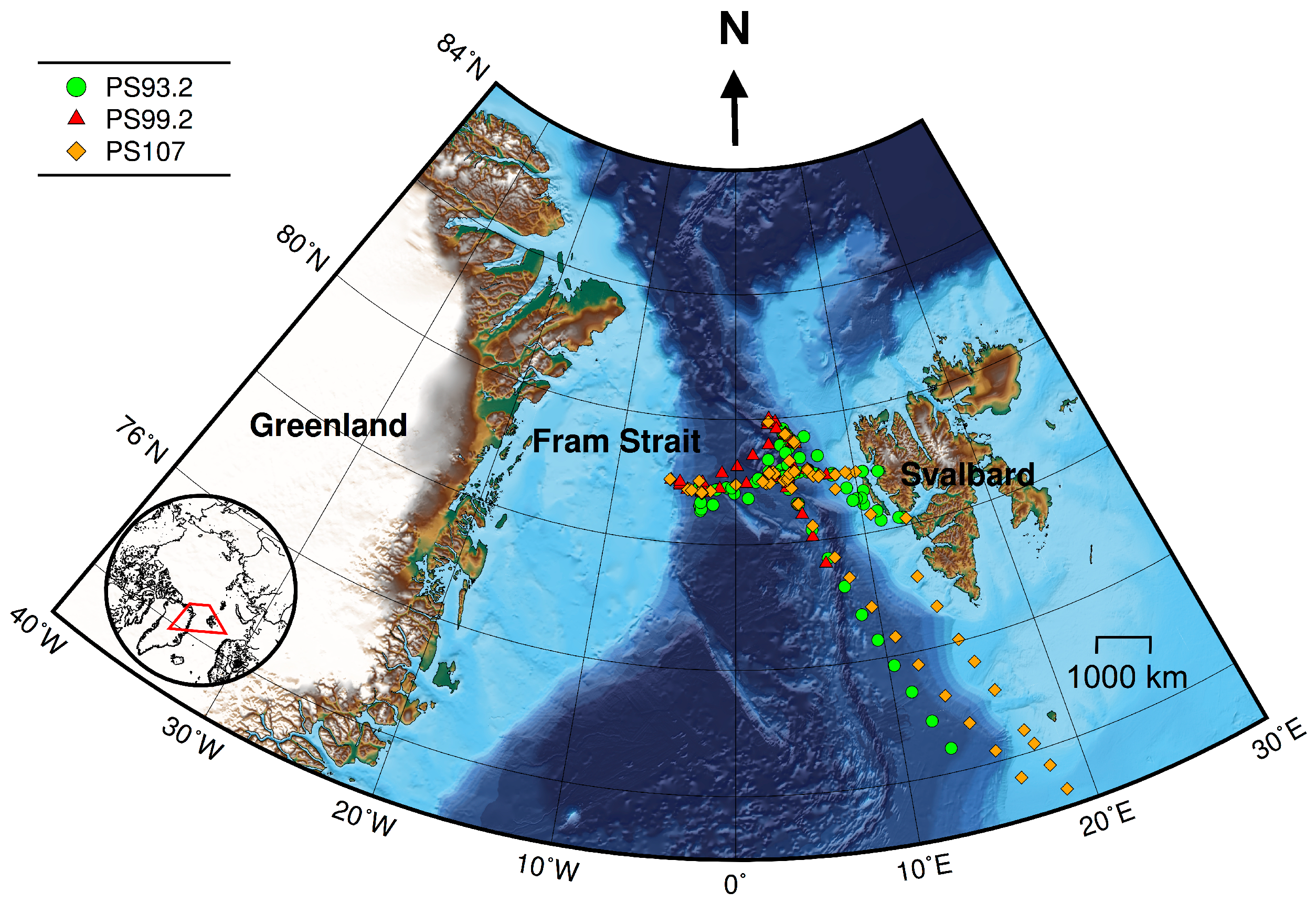
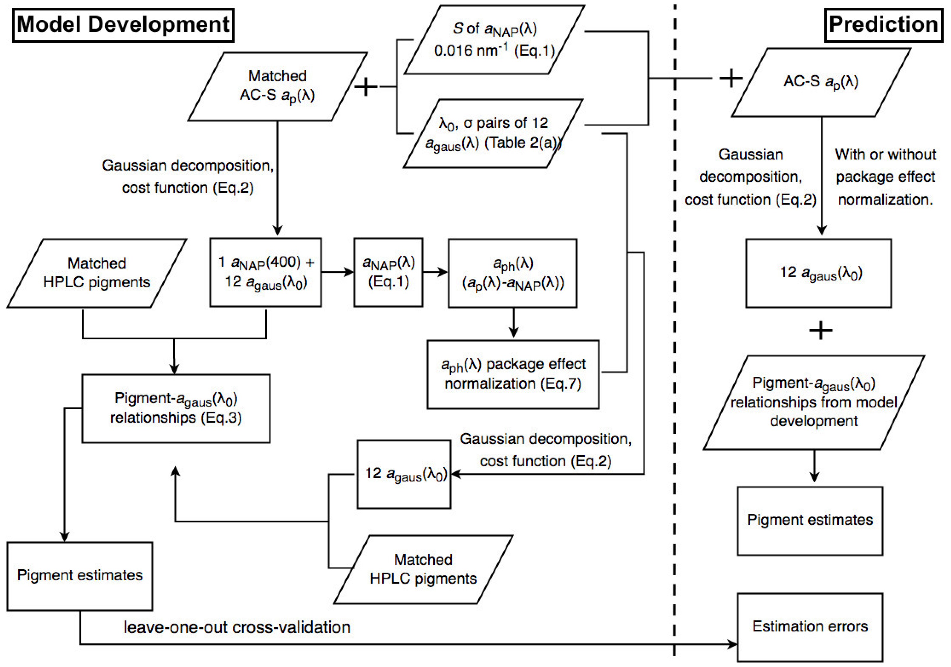
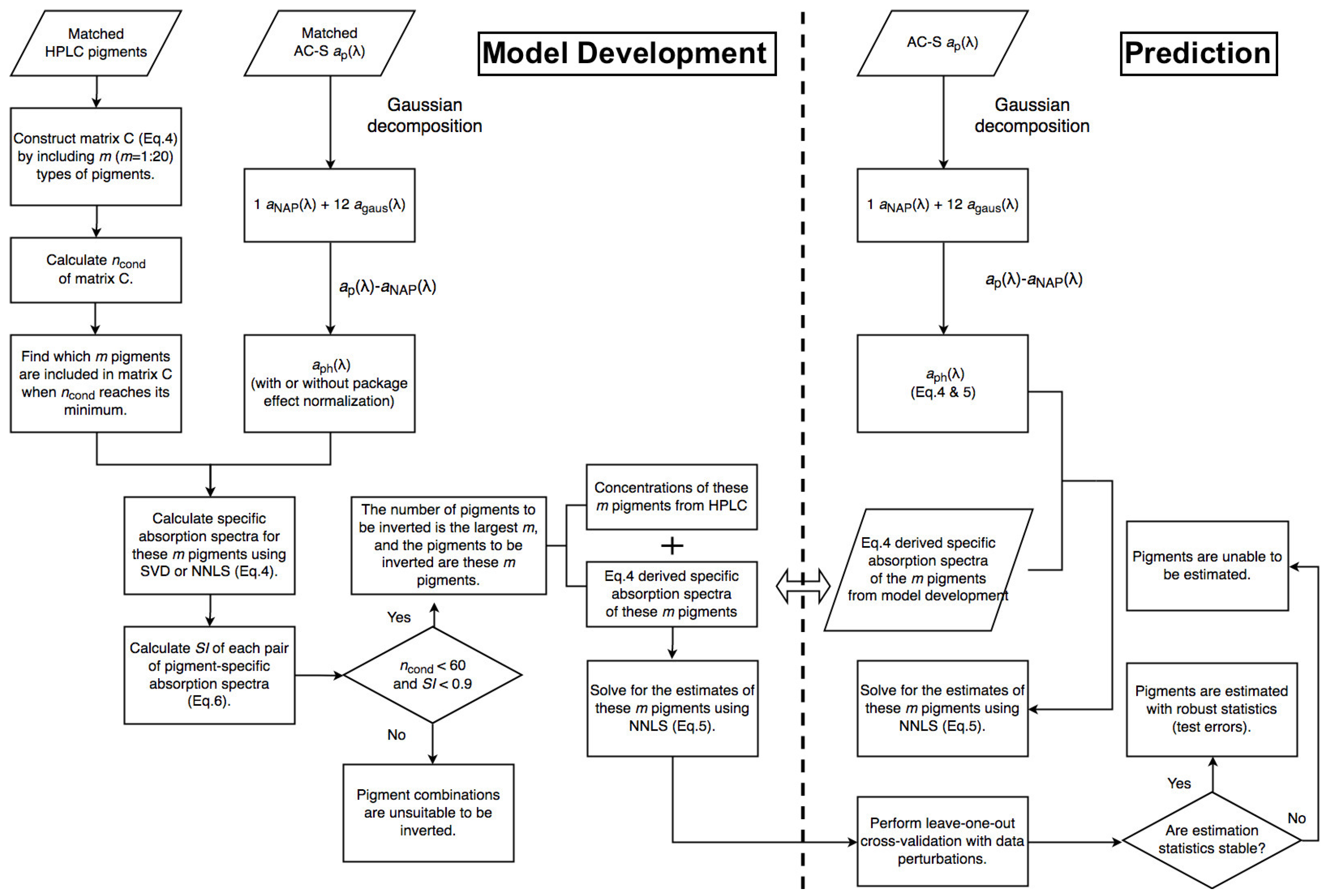
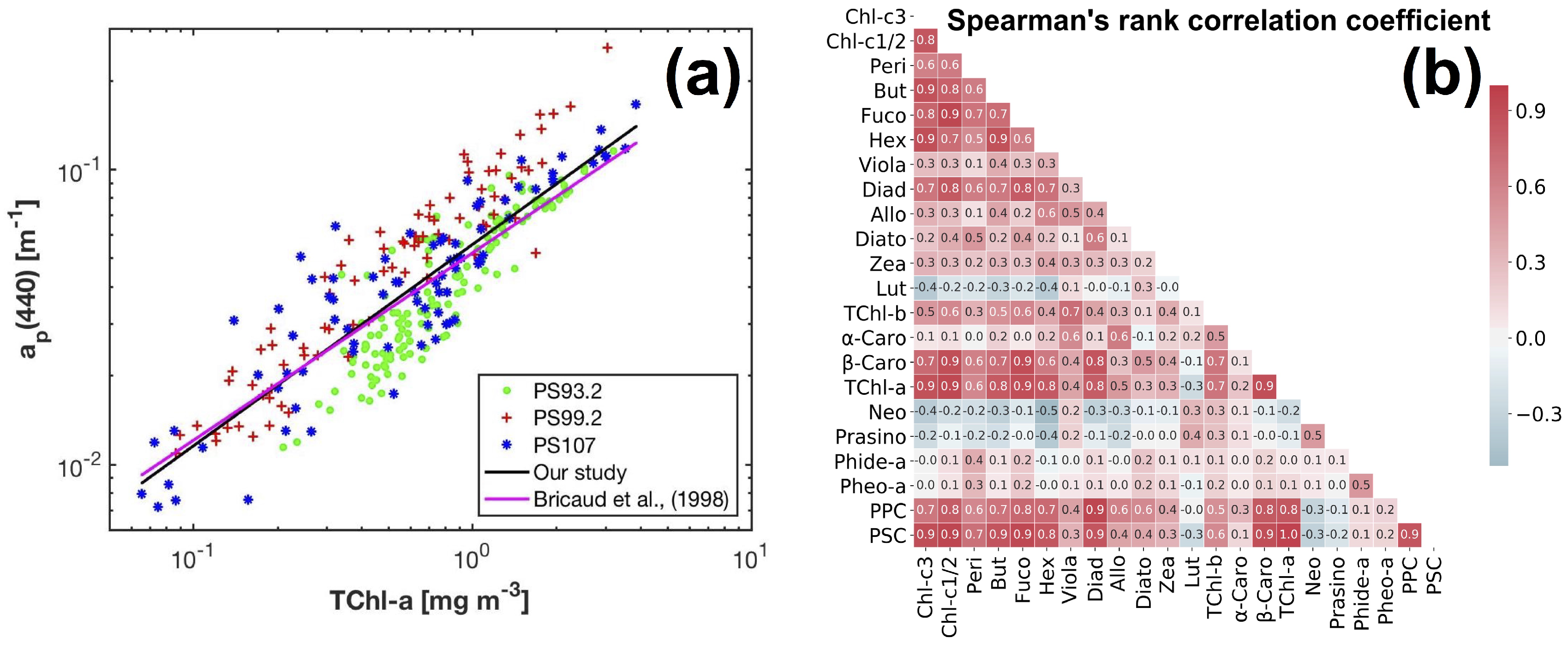
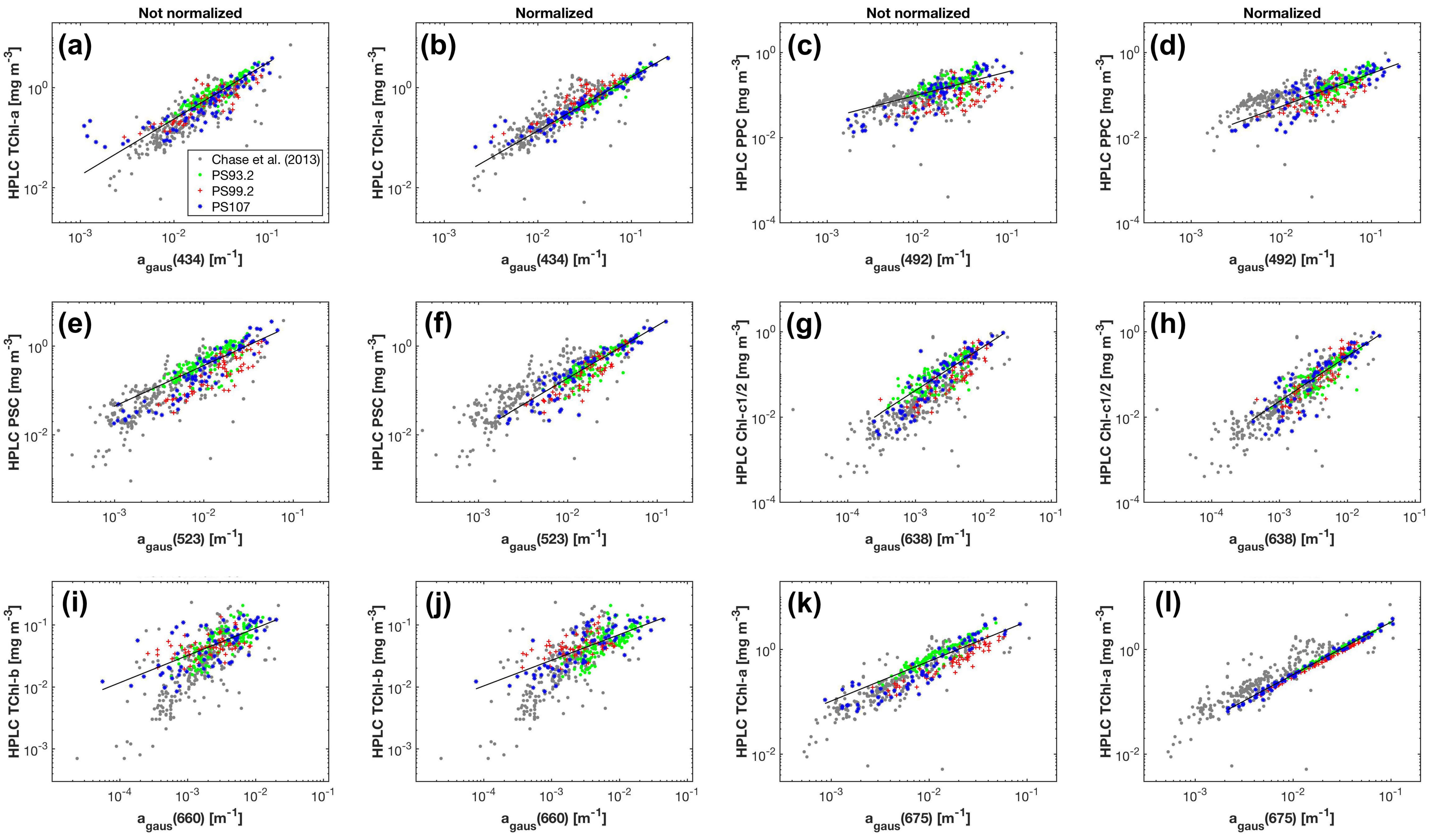
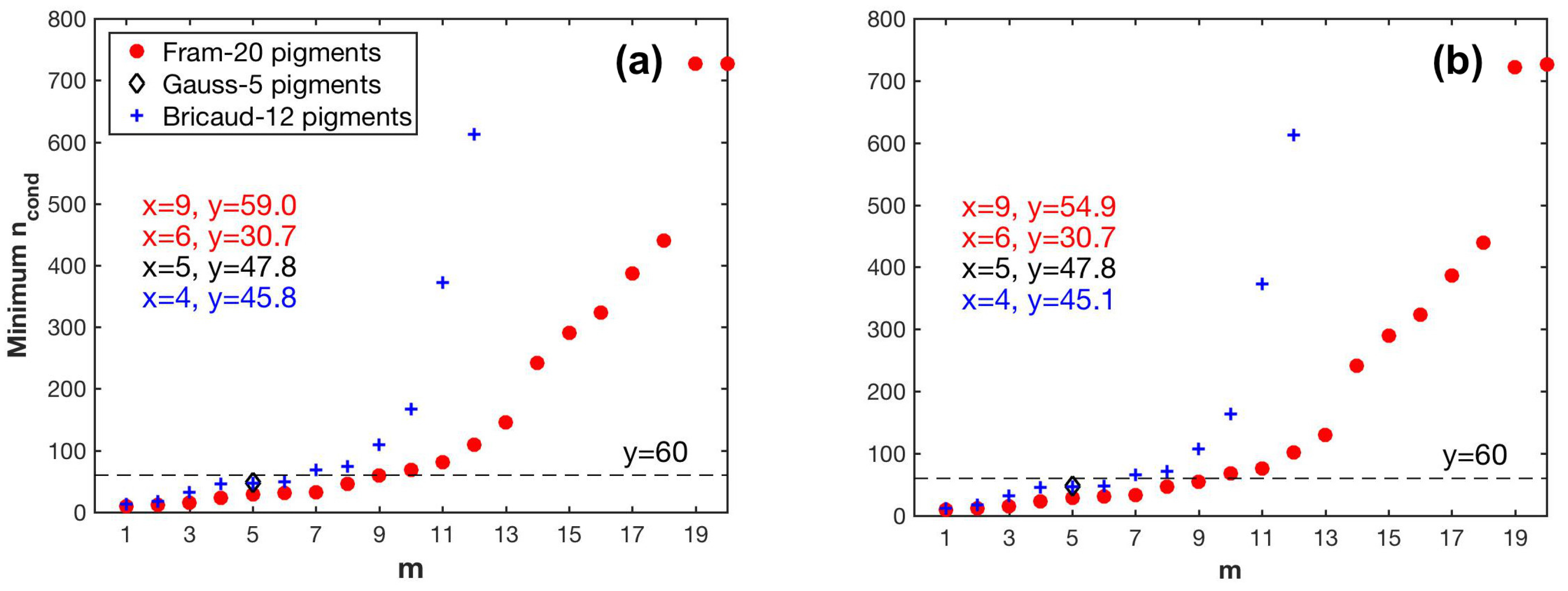
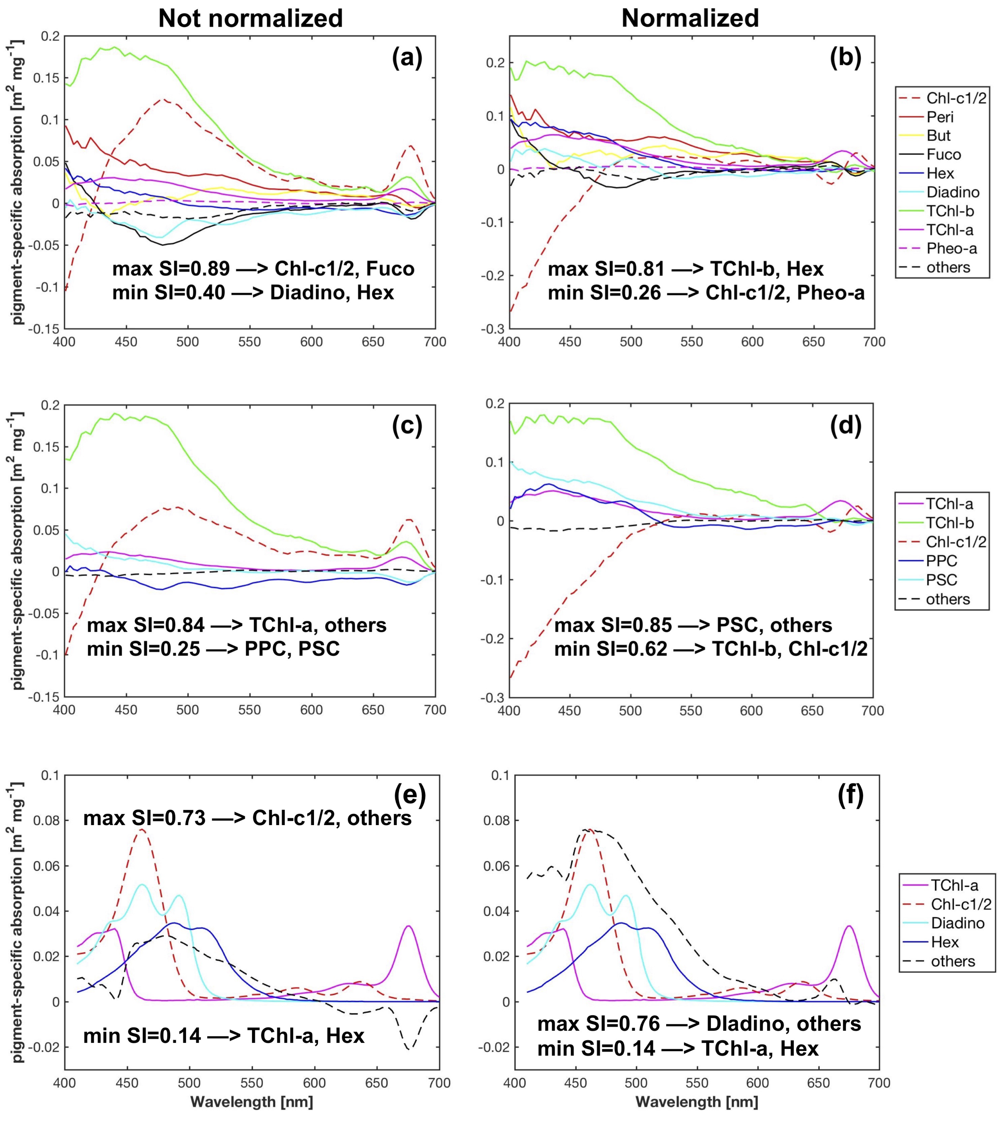
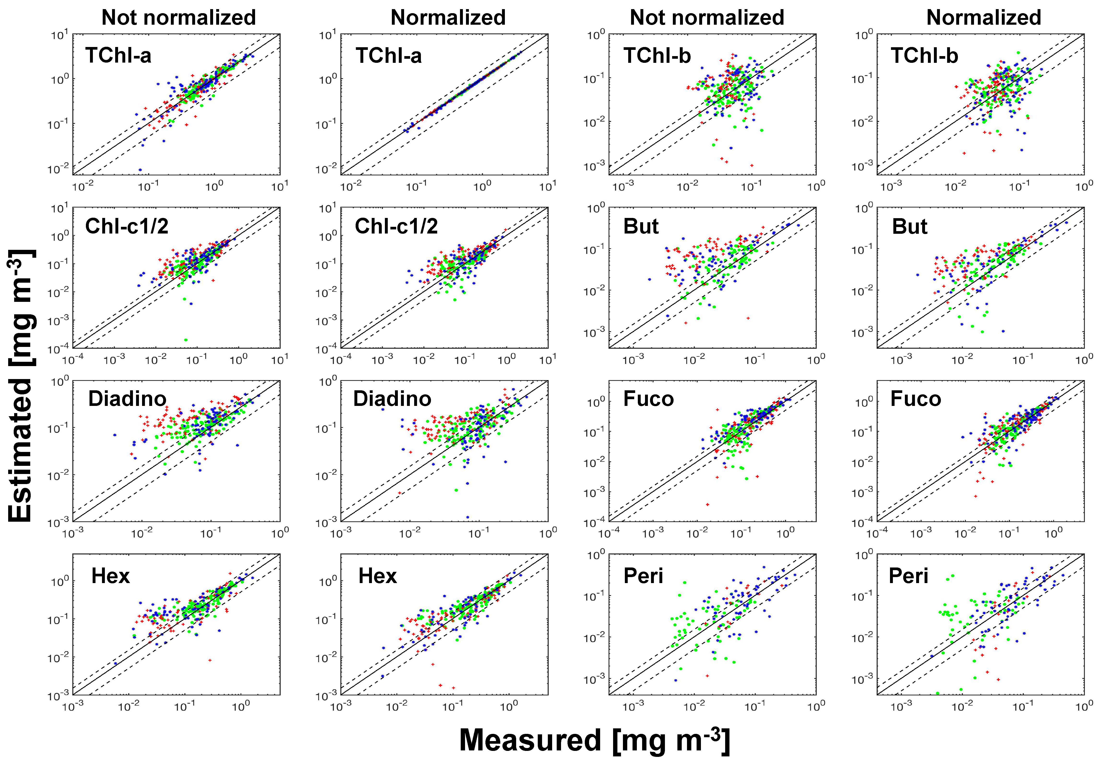
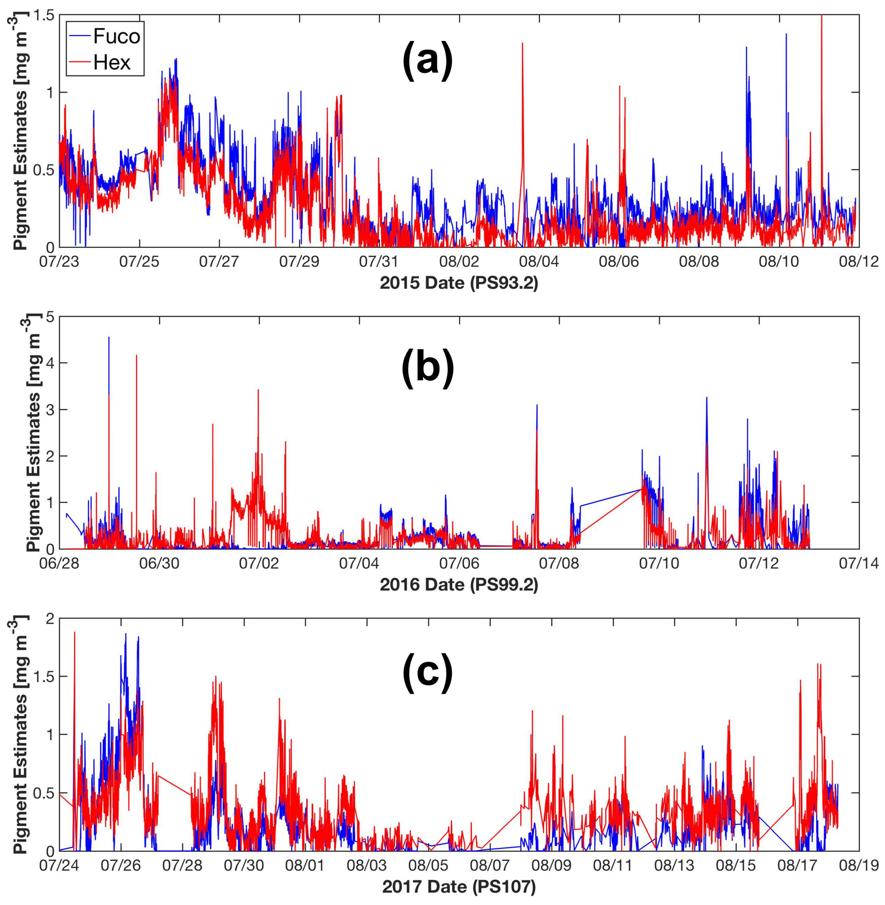
© 2019 by the authors. Licensee MDPI, Basel, Switzerland. This article is an open access article distributed under the terms and conditions of the Creative Commons Attribution (CC BY) license (http://creativecommons.org/licenses/by/4.0/).