Abstract
High-resolution maps of redwood distributions could enable strategic land management to satisfy diverse conservation goals, but the currently-available maps of redwood distributions are low in spatial resolution and biotic detail. Classification of airborne imaging spectroscopy data provides a potential avenue for mapping redwoods over large areas and with high confidence. We used airborne imaging spectroscopy data collected over three redwood forests by the Carnegie Airborne Observatory, in combination with field training data and application of a gradient boosted regression tree (GBRT) machine learning algorithm, to map the distribution of redwoods at 2-m spatial resolution. Training data collected from the three sites showed that redwoods have spectral signatures distinct from the other common tree species found in redwood forests. We optimized a gradient boosted regression model for high performance and computational efficiency, and the resulting model was demonstrably accurate (81–98% true positive rate and 90–98% overall accuracy) in mapping redwoods in each of the study sites. The resulting maps showed marked variation in redwood abundance (0–70%) within a 1 square kilometer aggregation block, which match the spatial resolution of currently-available redwood distribution maps. Our resulting high-resolution mapping approach will facilitate improved research, conservation, and management of redwood trees in California.
1. Introduction
Coastal redwoods (Sequoia sempervirens) are an exceptionally charismatic species. They are the tallest trees on earth, with some individuals taller than 100 m and older than 2000 years in age. Redwoods are endemic to the central coast of California and Southern Oregon, and redwood forests are locally- and globally-valued ecosystems [1]. Historically, redwoods have been an important source of lightweight, decay-resistant timber, and redwood logging remains an important source of revenue in some regions. Redwood forests are unique sites for recreation, and visitors to redwood-dominated state and national parks contribute $34 million dollars each year to local economies [1]. Redwoods have also been the focus of recent research interest due to their unique potential for carbon storage [2], with some redwood forests estimated to store 2600 mg of aboveground carbon per unit hectare, the highest values recorded on earth [3].
Given the multiple and diverse interests in redwoods within the state of California, strategic land management is needed to bolster conservation goals [1]. Redwood conservation has a long history in California, beginning with the founding of the first state park in 1901 following intensive and unregulated logging of old-growth redwoods during the second half of the eighteenth century. While some old-growth forests were protected, logging in many redwood forest regions in California continued until the 1970s, when the passing of the Endangered Species Act increased the cost of obtaining a permit to harvest redwoods [4]. Currently, approximately 90% of extant redwood forest is second-growth forest that has been logged at some point during the last two centuries. Redwood forests are fragmented by past harvest history and current land use pressures, and accordingly, there is a need for local-scale, high resolution management of redwood forest land. Maps of redwood distributions are currently available at 1-km spatial resolution, but due to the complex topography, geology, and climate of coastal California, the abundance and properties of redwoods can vary enormously within a 1 km2 area. Higher-resolution maps have not yet been produced due to the challenge of conducting field work to identify trees over large areas in topographically complex regions.
Remote sensing image analysis provides an array of potential tools for mapping vegetation properties [5]. Variation in sensor type, the spectral resolution of the sensor and the spatial resolution of the data have different applications. Passive sensors such as the Landsat Multispectral Scanner (MSS), have been used for mapping vegetation types at the community level and regional scales [6]. Active remote sensing has also been applied for wetland vegetation classification, for example through the identification of mangroves in Vietnam from the Advanced Land Observing Satellite Phased Array type L-band Synthetic Aperture Radar (ALOS PALSAR) data [7]. With imagery at higher spatial resolution, discrimination of individual tree species is possible. Sentinal-2A—a satellite multispectral spectrometer with 13 spectral bands, ranging from 10–60 m resolution—was used to map tree species with 65% overall accuracy in Germany [8]. QuickBird satellite data at less than 3-m resolution was used to map forty tree species with a kappa coefficients between 0.68 and 0.94 [9], and WorldView-2 satellite data at 2-m resolution was used to map 10 tree species in Austria with between 33 and 94% producer’s accuracies and 57–92% user’s accuracies [10].
Classification of imagery high in both spectral and spatial resolution has an especially effective approach for mapping of individual tree species across a multitude of environments. Airborne Visible/Infrared Imaging Spectrometer (AVIRIS) imagery, at 3.5 m resolution and including 224 bands, was used to map urban tree species in Southern California with 94% accuracy at the tree type level and 70% accuracy at the individual tree level [11]. Hyperspectral data including 214 bands at approximately 2-m resolution from the Carnegie Airborne Observatory (CAO) was used to map tree species in a tropical forest with 94–97% producer’s accuracy and 94–100% user’s accuracy [12]. Combining high-resolution hyperspectral data with structural attributes of species derived from LiDAR data has also yielded maps with high accuracy. Including LiDAR-derived height and canopy profile information improved producer’s accuracies by 5.1–11.6%, and user’s accuracies by 8.4–18.8% for mapping 11 trees species in Canada from Airborne Imaging Spectrometer for Applications (AISA) hyperspectral data at 2-m resolution and LiDAR data at 0.8 m resolution [13].
Tree species classifications from remotely-sensed imagery have been implemented with both parametric and nonparametric classification algorithms [14], however, recent approaches have focused on nonparametric machine learning (ML) algorithms because they have shown to be high-performing and efficient [15]. Support vector machine (SVM) is the most widely-used algorithm for tree species mapping from remotely-sensed data [14], however, artificial neural networks (ANN) [16] and decision-tree-based methods such as random forest (RF) [17,18] and gradient boosted regression trees (GBRT) have also been used [19]. For example, a recent comparison of SVM with an RF classifier for mapping multiple tree species in Muir Woods National Monument in California with AISA hyperspectral imagery found that the SVM produced slightly higher overall accuracy (95.02% for SVM and 92.91% for RF) [20]. Gradient boosted regression trees (GBRT) are similar to RF, however for GBRT, regression trees are fitted sequentially on observations that are modelled poorly by the existing set of trees, which has the potential to improve their performance [21]. GBRT have been used less frequently than RF thus far, but have performed well for species mapping in recent studies. For example, a recent study using GBRT to map giant sequoia trees from CAO hyperspectral imagery from the southern Sierra Nevada mountains in California yielded 95.2–98% overall accuracy [22], and a study comparing SVM with GBRT’s for detecting Ohi’a crowns infected with rapid Ohi’a death on Hawaii island found that using a combined SVM and GBRT approach yielded higher performance than either algorithm independently [19]. Other decision tree algorithms such as rotation forest [23] and logistic model tree algorithms [7] have recently been successfully applied for mapping mangrove species.
Here, using imaging spectroscopy data collected from the Carnegie Airborne Observatory (CAO) and field training data, we used the unique reflectance signatures of redwoods in a GBRT classification model to identify redwoods with high accuracy in hyperspectral images collected from three forests. We used a grid search to identify a GBRT model that minimizes false detections of redwoods while maintaining high computational efficiency for application on large datasets. We then applied this model to three coastal redwood forests in California, and compared its performance across three forests with multiple measures of model performance. We used the resulting maps to assess variability in redwood distributions at 10-m resolution and discussed its potential for advancing knowledge on redwood ecology and improving the efficiency of redwood conservation and management.
2. Materials and Methods
2.1. Study Sites
We focused our study on three redwood forests in Northern California. Big Basin is the southernmost site (122°35′W, 37°57′N), with a mean annual precipitation of 1093 mm and mean annual temperature of 14.72 °C, Muir Woods is the mid-latitude site with a mean annual precipitation of 1160 mm and a mean annual temperature of 13.96 °C (122°35′W, 37°57′N), and Jackson Forest is the northernmost site (123°35′W, 39°21′N), with a mean annual precipitation of 1214 mm and mean annual temperature of 13.14 °C [24]. All three sites have a rainy season in winter, and summers characterized by frequent fog cover [4]. The area of data collection coverage was largest at Jackson Forest, with a flight-box area of 261.41 km2, and smallest at Big Basin with a flight-box area of 27.66 km2. The area of flight coverage at Muir Woods was 52.16 km2. While all three forests contain areas of both old-growth and second-growth redwood forests, Jackson Forest is the only site with an active harvest operation. Portions of Big Basin were logged as recently as the 1980s, whereas Muir Woods is mostly older second-growth, with the most recent logging occurring in the early 1900s.
2.2. Airborne Data Acquisition
We collected imaging spectroscopy and Light Detection and Ranging (LiDAR) data over three redwood forests in July of 2016 using the CAO (Figure 1, Table 1). The CAO is an aircraft that carries a Visible-to-Shortwave Imaging Spectrometer (VSWIR) coaligned with a dual-channel LiDAR sensor [25]. Data collection was performed at altitude of 1000 m above ground level at Big Basin and 2000 m above ground level at Muir Woods and Jackson Forest, yielding 1-m resolution data at Big Basin and 2-m resolution data at Muir Woods and Jackson Forest. LiDAR returns were processed to a three-dimensional LiDAR point cloud with the position and orientation data collected from the GPS-Inertial Measurement System (IMU) navigation system on-board the CAO, and were further processed to digital surface maps of ground elevation, canopy surface elevation, and canopy height at 0.5- or 1-m resolution depending on the site using the LAStools software suite [25]. The VSWIR collected data from 349 to 2482 nm in 427 distinct channels at a 5-nm wavelength increment, determined as the full-width at half maximum of a Gaussian response function. To improve the signal-to-noise ratio prior to atmospheric correction, VSWIR data were reduced by averaging each pair of neighboring channels, yielding 214 channels at 10-nm increments.
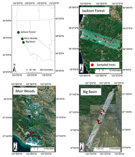
Figure 1.
Map of the three study sites and airborne spectroscopy and field data collected. The airborne imaging spectroscopy data are displayed for each site as a three-band RGB (red, green, and blue) composite image. The locations of individual field-collected data (including both training and testing data) are shown as red dots within each site. Field data were collected to cover each Carnegie Airborne Observatory flightline.

Table 1.
Date and time of Carnegie Airborne Observatory (CAO) airborne data acquisition and date of field data acquisition from each site.
2.3. Imaging Spectrometer Data Processing
The imaging spectroscopy data were radiometrically converted to radiance data with a flat field conversion and spectral calibration data, and were then ortho-georectified to the LiDAR surface elevation maps using the position and orientation data collected from the GPS-Inertial Measurement System (IMU) navigation system on-board the CAO [25]. The ACORN-6LX atmospheric correction model was then used to convert radiance to surface-level reflectance, with flight altitude and surface elevation inputs derived from the LiDAR data, and an internal Gaussian spectral response function (Imspec LLC, Glendale, California, USA). The ACORN-6LX visibility parameter specifies the atmospheric aerosol content at the time of data collection. A different visibility parameter was fit for each flightline of the reflectance data, in order to account for changes in atmospheric aerosols that occur throughout the day and thus vary across flightlines [19]. The visibility parameter was adjusted until the reflectance at 420 nm was 1%. Surface reflectance data from each flightline were mosaicked into a single image for each site. Prior to further analysis, reflectance data were filtered to remove the bands that primarily reflect absorption by atmospheric water vapor (1310–1460 nm and 1761–2021 nm) and at the upper and lower edges of the instrument detection limits (349–429 nm and 2432–2472 nm). We used the LAStools software package to produce a map of digital elevation and top-of-canopy height from the LiDAR point cloud data (Rapidlasso GmbH; Gilching, Germany). The top-of-canopy height map was then used with solar and viewing geometry data to identify pixels that were shaded at the time of the overflight, following prior work using CAO data [25,26,27].
2.4. Field Training Data Collection
Field data were collected from each of the three study sites from February–March, 2017, to identify pixels belonging to redwood trees and other species (Table 2). At each site, a tiled three-band composite of the reflectance data at 1–2-m resolution and top-of-canopy height images at 0.5–1-m resolution were loaded into the iGIS program on an iPad [28]. Individuals from each species were identified along trails at each of the three sites, and the pixels corresponding to those individuals were circled in the image. Training data were collected from at least 60 redwood trees and at least 60 individuals from the other common tree species at each site. Crowns were identified from at least 30 individuals of broadleaved trees, including tanoak (Lithocarpus densiflorus), madrone (Arbutus menziesii), and coast live oak (Quercus agrifolia), and at least forty Douglas fir (Pseudotsuga menziesii) trees at each site and five ponderosa pine trees at Big Basin. We collected additional training data from Douglas fir because they are the other commonly-occurring coniferous species in redwood forests, and we expected that they might show similar reflectance signatures to redwoods [20].

Table 2.
Sample sizes for the training and testing datasets for all three sites. Pixel values indicate the sample sizes input during the model development and testing. Values shown are the values following the masking of shaded and low-normalized difference vegetation index (NDVI) pixels.
Based on our observations in the field, location uncertainty of the iPad GPS could vary from 0 to 30 m, and sometimes exceeded the radius of individual tree crowns. We accounted for this in a variety of ways. First, we focused our collection to individuals that were easy to pick out in the combination of top-of-canopy height and RGB images because they were taller than their neighbors. We also identified adjacent individuals of the same species, so that we could identify groups of pixels >30 m in radius that belonged to same species, and we identified landmarks such as trails to aid in location triangulation in the field. To check our ability to collect good field training data with these approaches, we compared the reflectance of redwoods and Douglas fir (Figure A1 in Appendix A), two species that were similar in height, and often growing in mixed stands. We collected training data from redwoods and other species across all of the flightlines at each site, in order to minimize effects caused by differences in the visibility parameter of the atmospheric correction model (Figure 1).
Within each site, the dataset was then partitioned into a training dataset for classification model development and a testing dataset for classification model validation. Approximately 50% of redwood crowns from each site and fifty percent of crowns from other species from each site were placed into the testing dataset, with the remaining crowns placed into the training dataset. Crowns were randomly selected from the entire dataset of redwood crowns and other crowns, in order to ensure that the testing dataset and the training dataset were spatially distributed throughout the image. We combined the training data together from all three sites to build the classification model, and included a variable indicating the site in the model. Prior to further analysis, shaded pixels (identified by the LiDAR data as described above) and pixels with a normalized difference vegetation index (NDVI) of less than 0.7 [12], and pixels shorter than 2-m in height were removed from the dataset in order to remove shaded pixels and pixels with low leaf area [12,29]. We calculated NDVI using bands 35 (689.62 nm, near infrared) and 23 (569.45 nm, red) of the spectral data. The resulting sample size for training the model for was 6627 redwood pixels and 2816 other pixels for training, and 3249 redwood pixels and 2422 other pixels for testing. Sample sizes for each site are shown in Table 2.
2.5. Gradient Boosted Regression Tree Modeling
A gradient boosted regression tree (GBRT) model was used to classify pixels as either redwood pixels or other pixels. The GBRT is a decision-tree-based method, and it was selected because it effectively models nonlinear relationships, is a robust to predictor variables that have little to no influence on the response variable [21,30], and has worked well for past species mapping applications with CAO data [19,31,32]. In comparison with other ML algorithms for species mapping, GBRT also has the potential to show higher performance than random forest because each tree is fit on the residuals of the existing set of trees [21], and a combined GBRT-SVM approach showed higher performance for detecting trees infected with rapid Ohi’a death on Hawaii Island [19]. We performed a grid search across parameter combinations to select a model that was simultaneously high-performing and computationally-efficient. The parameters of a gradient boosted regression include the number of trees, the interaction depth, the subsample, the learning rate, the minimum number of samples at each leaf, and the loss function. To optimize model performance and efficiency, we varied the number of trees, the interaction depth, and the learning rate. Models with a higher number of trees will tend to show higher performance, but will also be less efficient [21]. The learning rate determines the extent to which each successive tree contributes to the resulting predictions, where a higher learning rate indicates that the first tree is substantially more important than the following trees. The interaction depth controls the number of nodes on each tree. With two nodes, the model can include two-way interactions among variables, and with three nodes, the model can incorporate three-way interactions, up to n nodes [21]. We searched across 33,750 parameter combinations, and calculated model performance through a ten-fold cross-validation at each combination of variables (Table 3). For each fold, the model was trained on a calibration set comprising 90% of the data, and tested on a validation set comprised of the remaining 10% of the data. In the cross-validation, pixels were grouped by crown identity, meaning that pixels from an individual crown could not end up in both the calibration set and the validation set. The validation accuracy thus returns the classification accuracy of tree crowns that do not have pixels included in the model calibration. All model development was done using the scikit learn package in Python [33].

Table 3.
Parameters of a gradient boosting regression and parameter values tested to find the best model. ‘Range’ specifies the maximum and minimum values of the parameter and number specifies the number of different values within that range that were tested.
While the data are binary, the GBRT model predicts a continuous variable, and a threshold value must be specified to produce a binary classification map. For each distinct combination of parameters, we calculated the true positive rate, also known as the sensitivity, and the false positive rate (equivalent to one minus the specificity) for one thousand distinct threshold values [34]. Our goal was to maintain a strictly low rate of false detections while maximizing the proportion of positive detections of redwoods, therefore, we used the true positive rate at a false positive rate of 2% as the performance criterion to evaluate model performance across parameter combinations. The true positive rate at a false positive rate of 2% was plotted as a function of the number of trees and the learning rate, with a separate plot for each interaction depth. To select the best model—a simultaneously high performing and highly efficient model—the interaction depth with the highest overall performance was selected, and we then chose the learning rate that yielded the highest performance at the lowest number of trees.
2.6. Model Application and Assessment
To assess model performance, we applied the chosen model to both the training dataset and the testing dataset for each site, and computed the true positive rate and false positive rate for one thousand distinct threshold values, and plotted a receiver operating characteristic curve (ROC). As the threshold values increase, both true positives and the false positives increase. Therefore, analysis of the ROC provides a measure of model performance across a range of possible threshold values [34]. We are aware of one prior study that has used analysis of ROC for vegetation mapping from remote sensing [35]. This is a distinct advantage of using a regression method for a binary classification problem rather than a classification method such as SVM: it enables the user to determine the threshold based on an application-specific measure of model performance. In our case, our goal was to minimize the proportion of other species that were classified as redwoods while maintaining a high redwood detection rate. To determine the threshold, we visually inspected the model predictions at each site in comparison with the field testing and training datasets (Figure A2), as well as the ROC curves, and selected a threshold that would minimize the false detections of other species as while maintaining a high redwood detection rate (Table A1). We applied the threshold to the training and testing data at each site, and then computed the true positive rate, false positive rate, overall accuracy, and Cohen’s Kappa test statistic for the training and testing datasets at all three sites.
The selected model was applied to each site, and the resulting redwood probability map was inspected visually to choose the best threshold for each site. The threshold was applied so that each pixel was classified as either a redwood or not a redwood. The true positive rate and false positive rate were then calculated for each site separately. We also applied a mask to remove shaded pixels and pixels with NDVI < 0.7, and pixels shorter than 2-m in height, as shaded and low-NDVI pixels had not been included in the training and testing datasets for model development and testing [12]. None of the data in the testing dataset had been used to perform the grid search; therefore, performance on the testing dataset provided an estimate of model performance in regions of the image where the training data had not been collected. A sieve filter (GDAL 201x) was then applied to pixels that were not touching more than three other pixels in order to remove isolated pixels that were too small to belong to whole crowns and may have been misclassified [12].
2.7. Calculation of Redwood Density and Redwood Height
Redwood crowns varied substantially in size. Prior studies have attempted to identify individual crowns through crown segmentation, with varying levels of accuracy [20,36,37]. However, due to the large size of our datasets, applying a crown segmentation algorithm would have been prohibitively computationally demanding. Rather than attempt to identify individual redwood crowns through crown segmentation, we resampled the redwood classification map to 10-m resolution to produce a map at a resolution that was approximately equal to the average crown size of a redwood. Redwood density was calculated as the proportion of 10-m pixels identified as a redwood within a 1 square kilometer aggregation block. We resampled the top-of-canopy height model to the same resolution by setting the 10-m resolution map equal to the maximum height of a 2-m pixel within a 10-m by 10-m pixel.
3. Results
3.1. Spectral Signatures of Redwoods
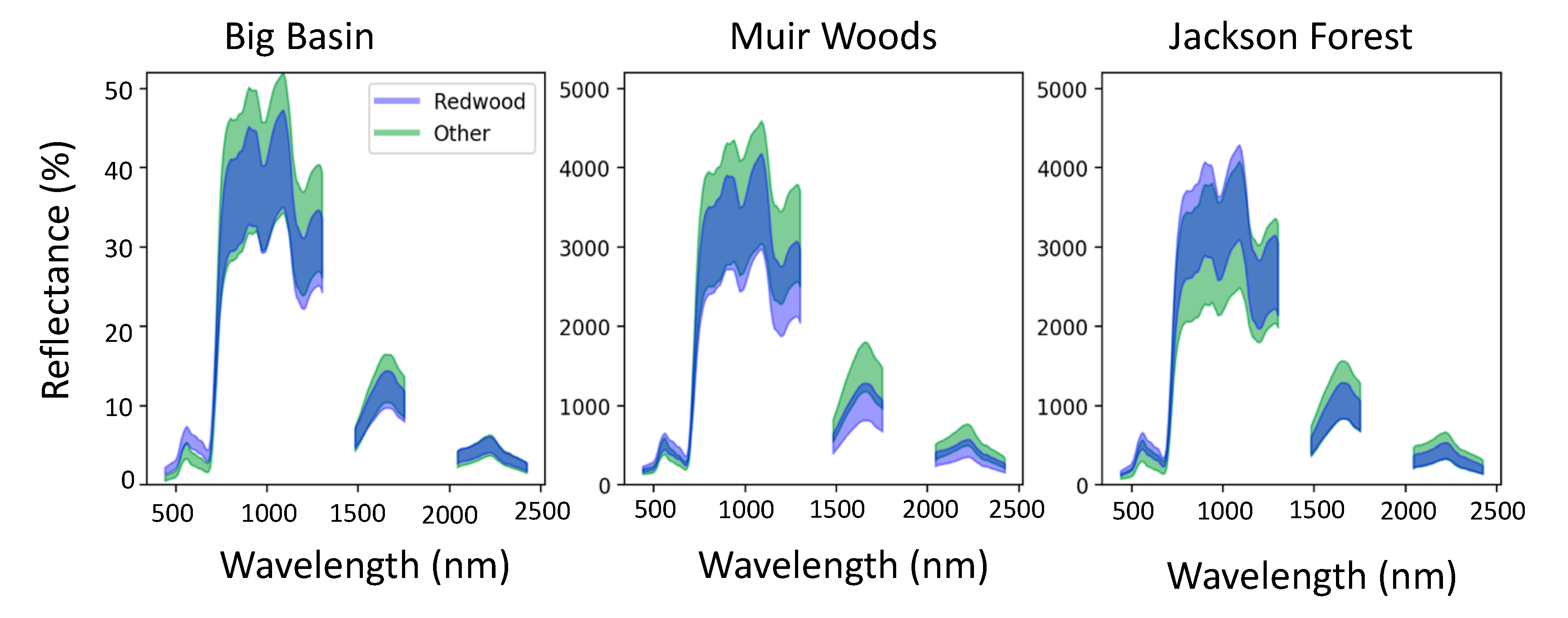
Redwoods were spectrally distinct from the other species in redwood forests (Figure 2) and the other common conifer species, Pseudotsuga menziesii (Douglas fir) (Figure A1). Across all sites, redwood pixels showed higher reflectance than the other species in the visible range, particularly from approximately 600 to 700 nm (Figure 2). In comparison with Douglas fir, the other common coniferous species found in redwood forests, redwood pixels showed higher reflectance in the visible range (400–700 nm) and also the near infrared range (NIR) (750–1100 nm) (Figure A1).

Figure 2.
The mean ± one standard deviation of spectral reflectance from redwoods (transparent blue) and other species (transparent green). Overlapping regions appear darker blue.
3.2. Model Optimization
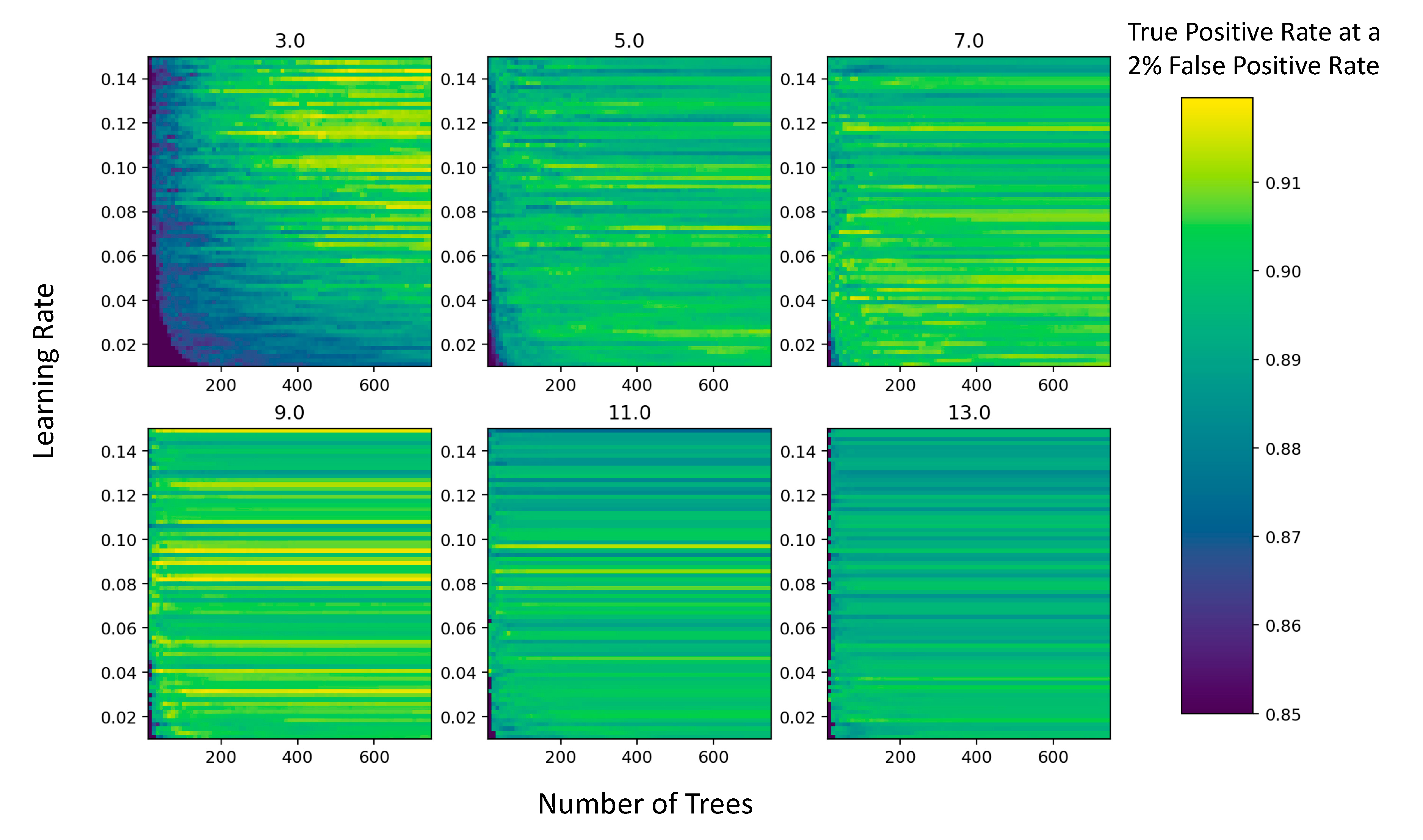
The model performance (calculated as the true positive rate at a given false positive rate) varied jointly as a function of the interaction depth, the learning rate, and the number of trees (Figure 3). While model performance tended to increase monotonically with increasing numbers of trees, the effect of varying the interaction depth (ID) on model performance was nonlinear (Figure 3). At the smallest interaction depth tested (ID = 3), we observed a trade-off in model performance between increasing the number of trees and increasing the learning rate (Figure 3). At higher interaction depth values (3 < ID < 13), the variation in model performance was more closely related to the value of the learning rate than the number of trees, except for very low numbers of trees which performed poorly (Figure 3). We also observed consistency in the model performance across a wide range of trees at some learning rates, exhibited by the horizontal bands of a single color in Figure 3. The model that yielded the highest performance at the smallest number of trees had a maximum depth of 9, a learning rate of 0.89, and 40 trees.
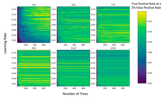
Figure 3.
Model performance as a function of the number of decision trees and the learning rate of the gradient boosted regression model. The color indicates the model performance, calculated as the true positive rate at a 2% false positive rate, of different gradient boosted regression models, plotted according to their interaction depth, the number of trees, and the learning rate. The different interaction depths vary among the plots and are shown as the title of the plot, the numbers of trees allowed in the model are the x-axes of all plots, and the learning rates are the y-axes of all plots.
3.3. Variation in True Positive Rate and False Positive Rate across the Sites
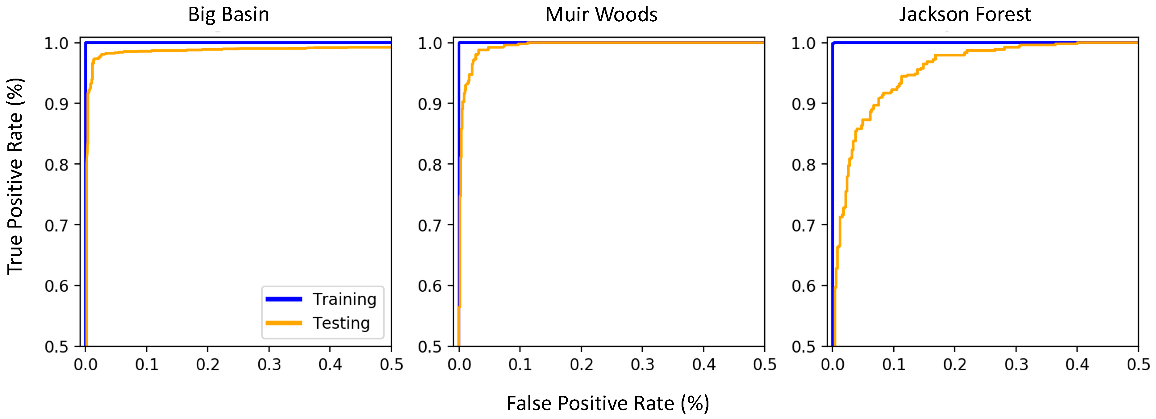
As we varied the threshold of the probability between zero and one, the true positive rate of the model increased sharply from zero to close to one, with very little increase in the false positive rate (Figure 4). As we continued to increase the threshold, the true positive rate increased marginally from 99% to almost 100% at Big Basin, 98% to almost 100% at Muir Woods, and 90% to almost 100% at Jackson Forest (Figure 4). The true positive rate and false positive rates of the final models selected varied across the sites (Table 4). When tested on the testing dataset that was not included in the model development, the final model with the thresholds selected by eye in each site yielded the highest true positive rate at Big Basin, and the lowest true positive rate at Jackson Forest. On the other hand, these models showed the lowest false positive rate at Muir Woods and the highest false positive rate at Jackson Forest. When tested on the training dataset on which the model was developed, the highest true positive rate observed was 100% at Muir Woods and all three sites showed a 0% false positive rate (Table 4). The difference in the true positive rate and the false positive rate between the training and the testing datasets was greatest at Jackson Forest, where the testing dataset showed significantly poorer performance than the training dataset (Table 4).
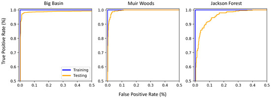
Figure 4.
Receiver operating characteristic curves for the final model for each site. Each point along the line is the true positive rate and false positive rate calculated when setting a distinct threshold value between zero and one, above which the pixel is classified as a redwood and below which it is classified as another species. Blue lines show the model performance evaluated on the training dataset and orange lines show the model performance evaluated on the testing dataset.

Table 4.
Four measures of model performance on the testing and the training datasets at all three sites.
3.4. Distribution of Redwood Density and Redwood Height
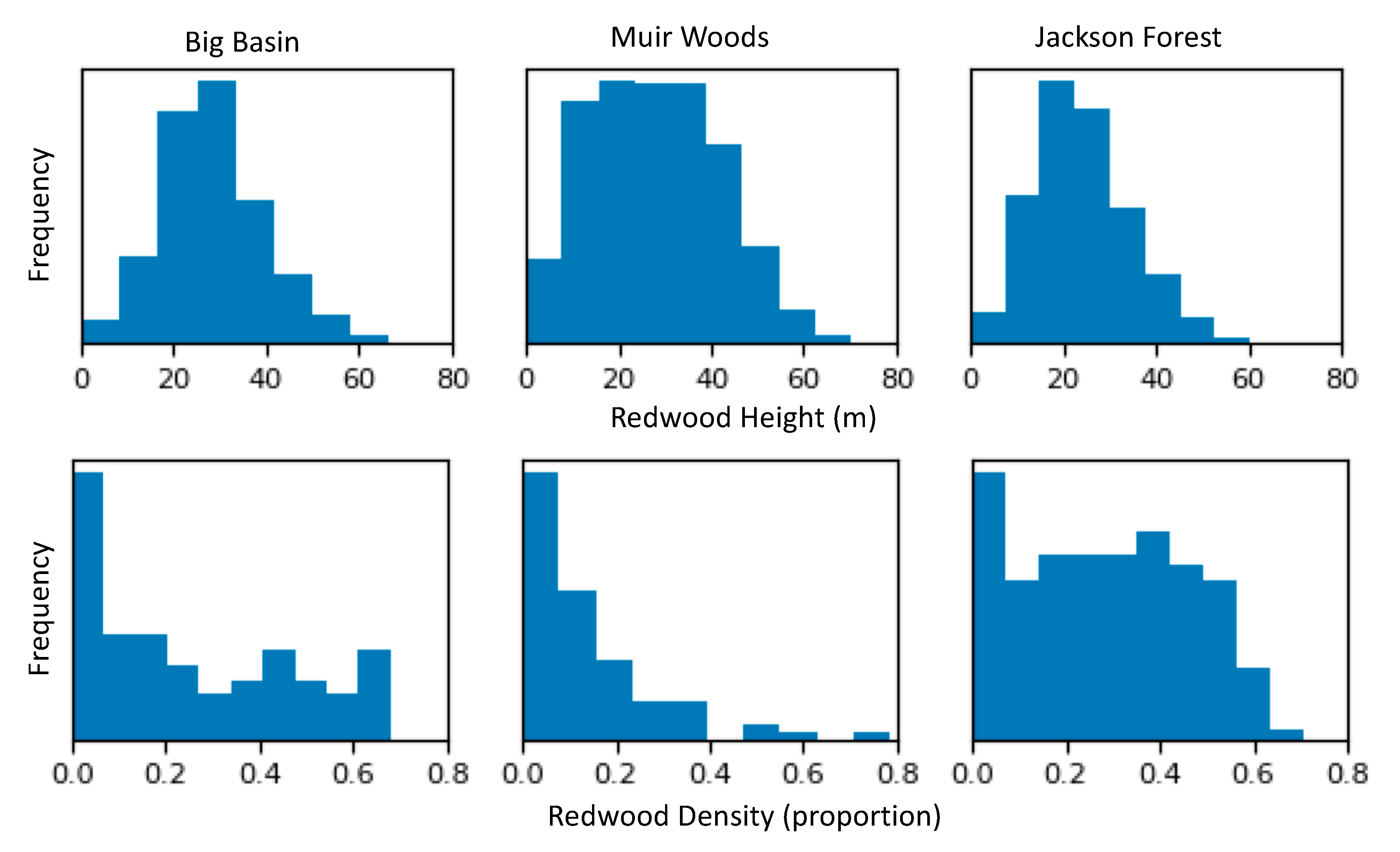
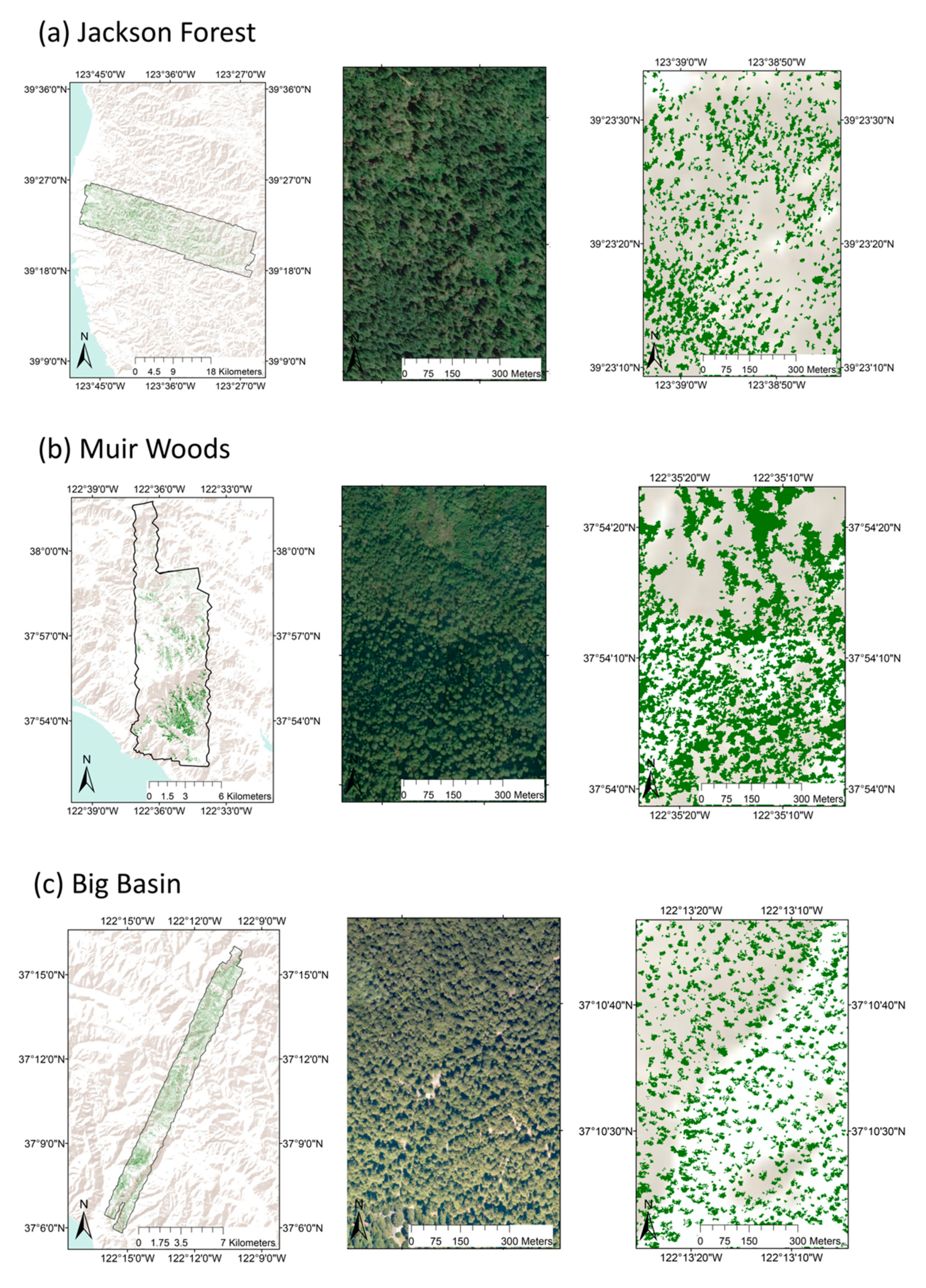
The distribution of redwood density within a 1 km2 grid cell was skewed (Figure 5). For all three sites, the most common redwood density value was close to zero, indicating a large proportion of area with no redwoods present. Big Basin showed an equivalently even distribution of area between 5 and 70% of redwoods, which can also be observed in the mapped crown images (Figure 6). On the other hand, Muir Woods showed a decline in frequency with increasing abundance, with more area with a lower redwood density, and only one 1 km2 grid cell with very high redwood density between 70 and 80%. Finally, the distribution of redwood density was the most uniform at Jackson Forest (Figure 5 and Figure 6). Although regions with redwood density of close to zero were the most frequent at Jackson Forest, regions with redwood density between approximately 5 and 55% were also commonly observed. The highest redwood density at Jackson Forest was 70%. The distribution of redwood height was close to normal in all three sites (Figure 5). The mean redwood height was close to 30 m at both Big Basin and Muir Woods, and the maximum redwood height was almost 80 m at both sites. Redwoods were shorter at Jackson Forest, with a mean redwood height at approximately 25 m, and a maximum redwood height of approximately 60 m (Figure 5).
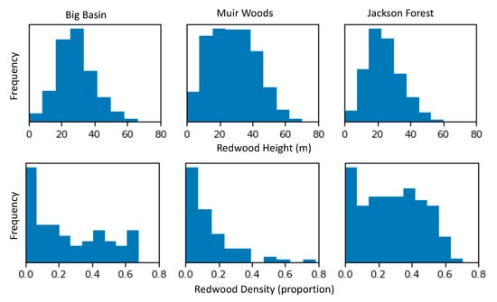
Figure 5.
Distributions of redwood height (top panel) and redwood density (bottom panel) at all three sites. Redwood height was calculated as the maximum height in a ten meter radius with a redwood in it; redwood density was calculated as the proportion of redwood detections within a 1-square kilometer aggregation block.
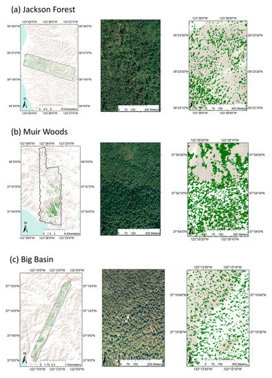
Figure 6.
Mapped redwood canopies for the three study sites. Canopies are shown mapped across the site (left column), and then shown in close-ups as google earth imagery (middle column), and then pixels identified by the model in the right column at the same location and resolution as the google earth imagery.
4. Discussion
4.1. Redwood Reflectance Signatures
The relatively higher reflectance of redwood pixels in the visible range (Figure 2), and higher reflectance of redwoods in comparison with Douglas fir in the NIR (Figure A1), can be interpreted in the context of their leaf chemistry. The visible range is a region where chemicals related to light capture and growth, specifically chlorophyll a, chlorophyll b, and carotenoids, interact with radiation [29,38], and higher reflectance in these regions indicates a higher concentration of these compounds in comparison with the other species. We also compared redwood reflectance with Douglas fir—the other tall coniferous species commonly found co-occurring with redwoods. The higher reflectance of redwood pixels in the near infrared region indicates higher canopy water content in redwood in comparison with Douglas fir, which is consistent with the higher capacity for water storage in redwood foliage in comparison with Douglas fir needles [39,40].
4.2. Model Selection and Parameterization
The improvement in the model performance with increasing interaction depth up to nine nodes (Figure 3) illustrates the importance of accounting for complex interactions among spectral bands when using high-dimensional hyperspectral data for species mapping. The trade-off in model performance between the number of trees and the learning rate at the smallest interaction depth (Figure 3) has been observed previously [21], and indicates that increasing the importance of the first tree in the resulting prediction becomes more important as the number of trees increases. The lack of a consistent relationship between the learning rate and the model performance may be due to the effect of the learning rate on the relative weighting of the trees. Since each tree in a GBRT is fit to a different randomly selected subset of data, changing the learning rate also changes the amount by which the first random subset of data sampled affects the model prediction, thereby resulting in the increased stochasticity we observed [21]. Boosted regression trees are fit sequentially, and an ensemble of GBRT trees can thus be made more efficient either by reducing the complexity of the individual trees [21] or by reducing the number of trees in the ensemble. We presented an example of the latter, and were able to identify a high-performing model at a very low number of trees, while accounting for complex interactions among spectral regions.
4.3. Model Performance
Overall accuracy was high, ranging from 90 to 98% depending on the site. This is similar to 91–95% for eight different species from a redwood forest [20] with Support Vector Machine, 25–95% when mapping urban tree species in Santa Barbara, California using Random Forest [41], 90–95% for mapping land cover classes in Vietnam using Random Forest [42], and between 55 and 95% for a range of coniferous tree species in Pacific Northwest forests in Canada using Support Vector Machine [43]. When reporting on measures of model performance that separate true positives and false negatives, we report true positive rates of 81–98% and false positive rates of 1–3%, depending on the site, in comparison with 82.5–99.7% and 0.6–3% for classifying tree crowns at different stages of pathogenic infection using gradient boosted regression in Hawaii [19], and 75–99% and 0–6% for classifying three large tree species in a tropical rainforest using an SVM [12].
In our study, we compared the performance of a single-species mapping algorithm across three study sites. We observed variation in model performance across the three sites and in particular, significantly lower performance, exhibited by a lower true positive rate (81% in comparison with 90% and 98%), a higher false positive rate (3% in comparison with 1% and 2%), lower overall accuracy (90% in comparison with 96% and 98%), and lower kappa statistic (0.81 in comparison with 0.90 and 0.95) at Jackson Forest in comparison with the other two sites. The lower performance at Jackson Forest is likely a result of its smaller average crown sizes and more heterogeneous canopy, which we hypothesize made it more difficult to obtain good field data for model development and testing. This is consistent with reports of lower overall accuracy for classification of tree species with smaller crown sizes in a prior urban tree species classification study [41]. Although all three of the sites in our study have a history of logging, Jackson Forest is the only site where logging is active, and also has the youngest stands, whereas both Muir Woods and Big Basin have a larger proportion of old-growth and older second-growth redwood forests. We also observed in the field and in the final redwood maps (Figure 6) that Jackson Forest was more heterogeneous, with more areas showing stands that were evenly mixed with redwoods and other species, in comparison with Big Basin and Muir Woods which tended to have large areas where a single species was dominant [20]. Small crown sizes and a heterogeneous canopy at Jackson Forest both lead to a greater frequency of mixed pixels, which are more difficult to classify [44]. Crown segmentation is cited as a potential solution to the problem of mixed pixels [45], but would have been prohibitively computationally demanding given the volume of data from Jackson Forest.
There are limitations to species mapping from airborne imaging spectroscopy and our approach in particular. By masking shaded pixels and pixels with NDVI less than 0.7, it is possible that there are some pixels that are a mix of both redwood foliage and either branches, bole, or soil that would not be classified in our map. For cases where these pixels are adjacent to pixels that are fully vegetated, this would not result in failure to identify redwood trees at the crown level. However, our algorithm is not able to identify redwood trees that are entirely shaded by other individuals or have NDVI less than 0.7 throughout their crowns.
4.4. Redwood Density and Height Patterns
Our resulting high-resolution redwood maps show marked variation in redwood forest density within a 1 square kilometer aggregation block. Current redwood distribution maps are available at 1 km2 resolution, and are presence-only, indicating whether a 1 km2 area is redwood forest or not [46]. Redwood density, calculated as the proportion of 10 m2 pixels classified as redwood within a 1 km2 aggregation block, varied from 0% redwood at many locations within all three sites, to greater than 70% redwoods at Muir Woods (Figure 5 and Figure 6). Although we did not perform a direct comparison of the coarse-resolution redwood maps with our high-resolution maps, the large variation in redwood density we reported suggests that there is likely to be substantial variation in redwood density in locations that are currently listed as homogenous redwood habitat in the 1 km2 resolution redwood distribution map. Prior comparisons of species density data with presence-only data have suggested that the ability to predict variation in species density from species presence-only data is context-dependent. While species abundance was consistently positively related to environmental suitability maps as predicted from species presence-only data in tropical and subtropical rainforests [47], it was weakly related across Amazonia [48]. Our results, which show large variation in redwood abundance from 0–70% within a 1 km2 aggregation block, are more consistent with the latter example.
The distribution in redwood height across the three sites reflects a combination of land-use history and environmental variability. Redwoods are a profitable timber species, and 90% of extant redwood forests are second-growth forests that have been logged at least once over the past two centuries. Both Muir Woods and Big Basin had some trees that were more than 70 m (230 feet) tall, whereas at Jackson Forest, the tallest redwoods observed were shorter than 60 m. Both Muir Woods and Big Basin have sections of old-growth forest in the areas where data was collected, whereas Jackson Forest is almost entirely comprised of second-growth forest, which explains why the maximum height of the trees is shorter. All of the forests had some trees that were below 10-m in height, which may reflect stands that were either very recently logged at Jackson Forest, or stunted redwoods growing in sites with poor water or nutrient availability.
4.5. Applications to Research, Conservation, and Management
High-resolution maps of redwood distribution and height will be useful in advancing research, conservation, and management of redwoods. High-resolution maps could be used in species distribution models for redwoods [49] to improve predictions on where redwoods will be resilient to future changes in fog and rainfall as a result of climate change [50,51]. High-resolution maps of redwoods could also be used to guide field studies of redwoods across environmental gradients. Redwood maps could be used by conservation organizations to identify priority areas for redwood conservation [52]. Finally, maps of redwood abundance and height could help to guide the management of redwood forests towards objectives such as carbon storage or restoration of old-growth forest characteristics [53]. While our data was limited to three regional sites, collection of airborne imaging spectroscopy and LiDAR data for the entirety of the redwood region to produce wall-to-wall maps would be time-intensive, highlighting the need for the development and deployment of high-resolution, spaceborne imaging spectroscopy instrumentation.
5. Conclusions
We showed that it is possible to map redwood tree canopies with 90–98% overall accuracy and high computational efficiency using airborne imaging spectroscopy data, field data on species identity, and gradient boosted regression trees. By analyzing reflectance signatures of pixels from redwoods and other species from the three study sites, we found that redwoods are spectrally differentiable from the neighboring tree species, with redwood reflectance signatures indicating greater investment in chemicals related to photosynthesis and water storage. We found reduced model performance at the site with the most active timber harvest history, which we suspect is due to resulting smaller tree crowns and higher frequency of mixed pixels. The resulting maps show variability in redwood density within a 1 square kilometer aggregation block of redwood forest from 0–70%, and pave the way for future high-resolution species distribution modeling of redwoods for scientific and management purposes.
Author Contributions
Conceptualization, E.F. and G.A.; Data Curation, G.A.; Formal Analysis, E.F.; Funding Acquisition, E.F. and G.A.; Investigation, E.F.; Methodology, E.F. and G.A.; Project Administration, E.F. and G.A.; Resources, G.A.; Software, E.F. and G.A.; Supervision, G.A.; Validation, E.F.; Visualization, E.F.; Writing—Original Draft, E.F.; Writing—Review & Editing, E.F. and G.A.
Funding
The Carnegie Airborne Observatory data collection and processing was funded by the David and Lucile Packard Foundation. E. J. Francis was supported by a Stanford Graduate Fellowship in Science and Engineering and field work expenses were supported by the Save the Redwoods League Grant #10674. The Carnegie Airborne Observatory has been made possible by grants and donations to G.P. Asner from the Avatar Alliance Foundation, Margaret A. Cargill Foundation, David and Lucile Packard Foundation, Gordon and Betty Moore Foundation, Grantham Foundation for the Protection of New Environments, W.M. Keck Foundation, John D. and Catherine T. MacArthur Foundation, Andrew Mellon Foundation Mary Anne Nyburt Baker, and G. Leonard Baker Jr. and William R. Hearst III.
Acknowledgments
We thank the staff of the Carnegie Airborne Observatory for assistance in data collection and processing. We thank Phil Brodrick for guidance on the optimization of the gradient boosted regression model, and for providing thoughtful comments on a draft of this manuscript. We thank Chris Field for his comments on a draft of this manuscript.
Conflicts of Interest
The authors declare no conflict of interest. The funders played no role in the choice of the research project, the design of the study, the collection, analyses, and interpretation of the data, the writing of the manuscript, or in the decision to publish the results.
Appendix A

Figure A1.
The mean ± one standard deviation of spectral reflectance from redwoods (Sequoia sempervirens) (transparent blue) and Douglas fir (Pseudotsuga menziesii) (transparent green). Overlapping regions appear darker blue.
Figure A1.
The mean ± one standard deviation of spectral reflectance from redwoods (Sequoia sempervirens) (transparent blue) and Douglas fir (Pseudotsuga menziesii) (transparent green). Overlapping regions appear darker blue.

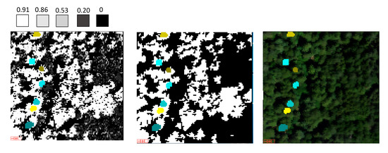
Figure A2.
The leftmost panels shows the gradient boosted regression tree (GBRT) output threshold map, with field-collected training and testing data shown in blue, green, and yellow colors. The middle map is the classification map once the threshold and the sieve had been applied, and the right map shows a red, green, and blue composite image of the same location, with the field-collected training and testing crowns shown in blue and yellow.
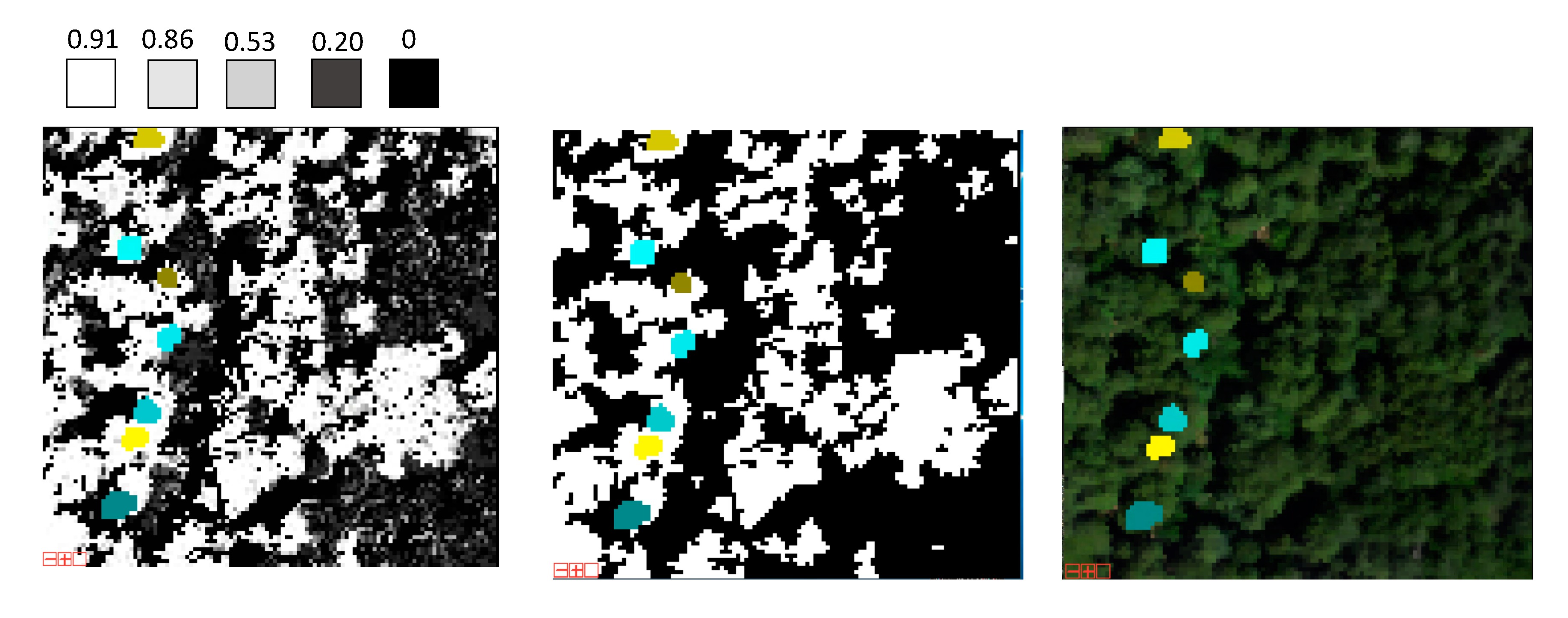

Table A1.
Threshold values selected for each site.
Table A1.
Threshold values selected for each site.
| Site | Big Basin | Muir Woods | Jackson Forest |
|---|---|---|---|
| Threshold Value | 0.76 | 0.69 | 0.80 |
References
- Burns, E.B.; Campbell, R.; Cowan, P.D. State of Redwoods Conservation Report: A Tale of Two Forests; Save the Redwoods League: San Francisco, CA, USA, 2018. [Google Scholar]
- Cameron, D.R.; Marvin, D.C.; Remucal, J.M.; Passero, M.C. Ecosystem management and conservation can substantially contribute to California’s climate mitigation goals. Proc. Natl. Acad. Sci. USA 2017, 114, 12833–12838. [Google Scholar] [CrossRef] [PubMed]
- Van Pelt, R.; Sillett, S.C.; Kruse, W.A.; Freund, J.A.; Kramer, R.D. Emergent crowns and light-use complementarity lead to global maximum biomass and leaf area in Sequoia sempervirens forests. For. Ecol. Manag. 2016, 375, 279–308. [Google Scholar] [CrossRef]
- Noss, R.F. (Ed.) The Redwood Forest: History, Ecology, and Conservation of the Coast Redwoods; Island Press: Washington, DC, USA, 2000. [Google Scholar]
- Franklin, J. Predictive vegetation mapping: Geographic modelling of biospatial patterns in relation to environmental gradients. Prog. Phys. Geogr. 1995, 19, 474–499. [Google Scholar] [CrossRef]
- Xie, Y.; Sha, Z.; Yu, M. Remote sensing imagery in vegetation mapping: A review. J. Plant Ecol. 2008, 1, 9–23. [Google Scholar] [CrossRef]
- Pham, T.D.; Bui, D.T.; Yoshino, K.; Nhu Le, H. Optimized rule-based logistic model tree algorithm for mapping mangrove species using ALOS PALSAR imagery and GIS in the tropical region. Environ. Earth Sci. 2018, 77, 1–13. [Google Scholar] [CrossRef]
- Immitzer, M.; Francesco, V.; Atzberger, C. First Experience with Sentinel-2 Data for Crop and Tree Species Classifications in Central Europe. Remote Sens. 2016, 8, 166. [Google Scholar] [CrossRef]
- Lin, C.; Popescu, S.C.; Thomson, G.; Tsogt, K.; Chang, C. Classification of Tree Species in Overstory Canopy of Subtropical Forest Using Quickbird Images. PLoS ONE 2015, 10, e0125554. [Google Scholar]
- Immitzer, M.; Atzberger, C.; Koukal, T. Tree Species Classification with Random Forest Using Very High Spatial Resolution 8-Band WorldView-2 Satellite Data. Remote Sens. 2012, 4, 2661–2693. [Google Scholar] [CrossRef]
- Alonzo, M.; Roth, K.; Roberts, D. Identifying Santa Barbara’s urban tree species from AVIRIS imagery using canonical discriminant analysis. Remote Sens. Lett. 2013, 4, 513–521. [Google Scholar] [CrossRef]
- Baldeck, C.A.; Asner, G.P.; Martin, R.E.; Anderson, C.B.; Knapp, D.E.; Kellner, J.R.; Wright, S.J. Operational Tree Species Mapping in a Diverse Tropical Forest with Airborne Imaging Spectroscopy. PLoS ONE 2015, 10, e0118403. [Google Scholar] [CrossRef]
- Jones, T.G.; Coops, N.C.; Sharma, T. Assessing the utility of airborne hyperspectral and LiDAR data for species distribution mapping in the coastal Pacific Northwest. Remote Sens. Environ. 2010, 114, 2841–2852. [Google Scholar] [CrossRef]
- Fassnacht, F.E.; Latifi, H.; Stere´nczak, K.; Modzelewska, A.; Lefsky, M.; Waser, L.T.; Straub, C.; Ghosh, A. Review of studies on tree species classification from remotely sensed data. Remote Sens. Environ. 2016, 186, 64–87. [Google Scholar] [CrossRef]
- Maxwell, A.E.; Warner, T.A.; Fang, F. Implementation of machine-learning classification in remote sensing: An applied review. Int. J. Remote Sens. 2018, 39, 2784–2817. [Google Scholar] [CrossRef]
- Zhang, C.; Xie, Z. Combining object-based texture measures with a neural network for vegetation mapping in the Everglades from hyperspectral imagery. Remote Sens. Environ. 2012, 124, 310–320. [Google Scholar] [CrossRef]
- Belgiu, M.; Drăgut, L. Random forest in remote sensing: A review of applications and future directions. ISPRS J. Photogramm. Remote Sens. 2016, 114, 24–31. [Google Scholar] [CrossRef]
- Amini, S.; Homayouni, S.; Safari, A.; Darvishsefat, A.A. Object-based classification of hyperspectral data using Random Forest algorithm. Geo-Spat. Inf. Sci. 2018, 21, 127–138. [Google Scholar] [CrossRef]
- Vaughn, N.R.; Asner, G.P.; Brodrick, P.G.; Martin, R.E.; Heckler, J.W.; Knapp, D.E.; Hughes, R.F. An approach for High-Resolution Mapping of Hawaiian Metrosideros Forest Mortality Using Laser-Guided Imaging Spectroscopy. Remote Sens. 2018, 10, 502. [Google Scholar] [CrossRef]
- Ballanti, L.; Blesius, L.; Hines, E.; Kruse, B. Tree Species Classification Using Hyperspectral Imagery: A Comparison of Two Classifiers. Remote Sens. 2016, 8, 445. [Google Scholar] [CrossRef]
- Elith, J.; Leathwick, J.R.; Hastie, T. A working guide to boosted regression trees. J. Anim. Ecol. 2008, 77, 802–813. [Google Scholar] [CrossRef]
- Paz-Kagan, T.; Brodrick, P.G.; Vaughn, N.R.; Das, A.J.; Stephenson, N.L.; Nydick, K.R.; Asner, G.P. What mediates tree mortality during drought in the southern Sierra Nevada? Ecol. Appl. 2017, 27, 2443–2457. [Google Scholar] [CrossRef]
- Zhang, H.; Wang, T.; Liu, M.; Jia, M.; Lin, H.; Chu, L.; Devlin, A. Potential of combining optical and dual polarimetric sar data for improving mangrove species discrimination using rotation forest. Remote Sens. 2018, 10, 467. [Google Scholar] [CrossRef]
- Daly, C.; Taylor, G.H.; Gibson, W.P.; Parzybok, T.W.; Johnson, G.L.; Pasteris, P.A. High-Quality Spatial Climate Data Sets for the United States and Beyond; Group, P.C., Ed.; Oregon State University: Corvallis, OR, USA, 2017. [Google Scholar]
- Asner, G.P.; Knapp, D.E.; Boardman, J.; Green, R.O.; Kennedy-Bowdown, T.; Eastwood, M.; Martin, R.E.; Anderson, C.; Field, C.B. Carnegie Airborne Observatory-2: Increasing science data dimensionality via high-fidelity multi-sensor fusion. Remote Sens. Environ. 2012, 124, 454–465. [Google Scholar] [CrossRef]
- Asner, G.P.; Knapp, D.E.; Kennedy-Bowdown, T.; Jones, M.O.; Martin, R.E.; Boardman, J.; Field, C.B. Carnegie Airborne Observatory: In-flight fusion of hyperspectral imaging and waveform light detection and ranging for three-dimensional studies of ecosystems. J. Appl. Remote Sens. 2007. [Google Scholar] [CrossRef]
- Asner, G.; Martin, R. Spectral and chemical analysis of tropical forests: Scaling from leaf to canopy levels. Remote Sens. Environ. 2008, 112, 3958–3970. [Google Scholar] [CrossRef]
- Marvin, D.C.; Asner, G.P.; Schnitzer, S.A. Liana canopy cover mapped throughout a tropical forest with high-fidelity imaging spectroscopy. Remote Sens. Environ. 2016, 176. [Google Scholar] [CrossRef]
- Asner, G.P.; Martin, R.E.; Anderson, C.B.; Knapp, D.E. Quantifying forest canopy traits: Imaging spectroscopy versus field survey. Remote Sens. Environ. 2015, 158, 15–27. [Google Scholar] [CrossRef]
- Friedman, J.H. 1999 Reitz Lecture: Greedy Function Approximation: A Gradient Boosting Machine. Ann. Stat. 2001, 29, 1189–1232. [Google Scholar] [CrossRef]
- Paz-Kagan, T.; Vaughn, N.R.; Martin, R.E.; Brodrick, P.G.; Stephenson, N.L.; Das, A.J.; Nydick, K.R.; Asner, G.P. Landscape-scale variation in canopy water content of giant sequoias during drought. For. Ecol. Manag. 2018, 419–420, 291–304. [Google Scholar] [CrossRef]
- Niemiec, R.M.; Asner, G.P.; Brodrick, P.G.; Gaertner, J.A.; Ardoin, N.M. Scale-dependence of environmental and socioeconomic drivers of albizia invasion in Hawaii. Landsc. Urban Plan. 2018, 169, 70–80. [Google Scholar] [CrossRef]
- Pedregosa, F.; Varoquax, G. Scikit-learn: Machine learning in Python. J. Mach. Learn. Res. 2011, 12. [Google Scholar]
- Fawcett, T. An introduction to ROC analysis. Pattern Recognit. Lett. 2006, 27, 861–874. [Google Scholar] [CrossRef]
- Alatorre, L.C.; Sánchez-Andrés, R.; Cirujano, S.; Beguería, S.; Sánchez-Carrillo, S. Identification of Mangrove Areas by Remote Sensing: The ROC Curve Technique Applied to the Northwestern Mexico Coastal Zone Using Landsat Imagery. Remote Sens. 2011, 3, 1568–1583. [Google Scholar] [CrossRef]
- Koch, B.; Heyder, U.; Weinacker, H. Detection of individual tree crowns in airborne lidar data. Photogramm. Eng. Remote Sens. 2006, 72. [Google Scholar] [CrossRef]
- Vauhkonen, J.; Ene, L.; Gupta, S.; Heinzel, J.; Holmgren, J.; Pitkanen, J.; Solberg, S.; Wang, Y.; Weinacker, H.; Hauglin, K.M.; et al. Comparative testing of single-tree detection algorithms under different types of forest. Forestry 2012, 85, 27–40. [Google Scholar] [CrossRef]
- Asner, G.P. Hyperspectral Remote Sensing of Canopy Chemistry, Physiology, and Biodiversity in Tropical Rainforests. In Hyperspectral Remote Sensing of Tropical and Sub-Tropical Forests; Sanchez-Azofeifa, M.K.a.G.A., Ed.; Taylor & Francis Group: Boca Raton, FL, USA, 2008. [Google Scholar]
- Ishii, H.R.; Azuma, W.; Kuroda, K.; Sillett, S.C.; Watling, J. Pushing the limits to tree height: Could foliar water storage compensate for hydraulic constraints in Sequoia sempervirens? Funct. Ecol. 2014, 28, 1087–1093. [Google Scholar] [CrossRef]
- Woodruff, D.R.; Bond, B.J.; Meinzer, F.C. Does turgor limit growth in tall trees? Plant Cell Environ. 2004, 27, 229–236. [Google Scholar] [CrossRef]
- Alonzo, M.; Bookhagen, B.; Roberts, D.A. Urban tree species mapping using hyperspectral and lidar data fusion. Remote Sens. Environ. 2014, 148, 70–83. [Google Scholar] [CrossRef]
- Noi, P.T.; Kappas, M. Comparison of Random Forest, k-Nearest Neighbor, and Support Vector Machine Classifiers for Land Cover Classification Using Sentinel-2 Imagery. Sensors 2018, 18, 18. [Google Scholar]
- Jones, T.G.; Coops, N.C.; Sharma, T. Assessing the utility of airborne hyperspectral and LiDAR data for species distribution mapping in the coastal Pacific Northwest, Canada. Remote Sens. Environ. 2010, 114, 2841–2852. [Google Scholar] [CrossRef]
- Hsieh, P.F.; Lee, L.C.; Chen, N.Y. Effect of Spatial Resolution on Classification Errors of Pure and Mixed Pixels in Remote Sensing. IEEE Trans. Geosci. Remote Sens. 2001, 39, 2657–2663. [Google Scholar] [CrossRef]
- Myint, S.W.; Gober, P.; Brazel, A.; Grossman-Clarke, S.; Weng, Q. Per-pixel vs. object-based classification of urban land cover extraction using high spatial resolution imagery. Remote Sens. Environ. 2011, 115, 1145–1161. [Google Scholar] [CrossRef]
- Griffin, J.R.; Critchfield, W.B. The Distribution of Forest Trees in California; US Department of Agriculture: Berkeley, CA, USA, 1976; pp. 1–115.
- VanDerWal, J.; Shoo, L.P.; Johnson, C.N.; Williams, S.E. Abundance and the environmental niche: Environmental suitability estimated from niche models predicts the upper limit of local abundance. Am. Nat. 2009, 174, 282–291. [Google Scholar] [CrossRef] [PubMed]
- Gomes, V.H.F.; Raes, N.; Amaral, I.L.; Salomao, R.P.; de Souza Coelho, L.; de Almeida Matos, F.D.; Castilho, C.V.; de Andrade Lima Filho, D.; Lopez, D.C.; Guevara, J.E.; et al. Species Distribution Modelling: Contrasting presence-only models with plot abundance data. Sci. Rep. 2018, 8, 1003. [Google Scholar] [CrossRef] [PubMed]
- Fernandez, M.; Hamilton, H.H.; Kueppers, L.M. Back to the future: Using historical climate variation to project near-term shifts in habitat suitability for coast redwood. Glob. Change Biol. 2015, 21, 4141–4152. [Google Scholar] [CrossRef] [PubMed]
- Johnstone, J.A.; Dawson, T.E. Climatic context and ecological implications of summer fog decline in the coast redwood region. Proc. Natl. Acad. Sci. USA 2010, 107, 4533–4538. [Google Scholar] [CrossRef] [PubMed]
- Diffenbaugh, N.S.; Swain, D.L.; Touma, D. Anthropogenic warming has increased drought risk in California. Proc. Natl. Acad. Sci. USA 2015, 112, 3931–3932. [Google Scholar] [CrossRef] [PubMed]
- Wulder, W.A.; Hall, R.J.; Coops, N.C.; Franklin, S.E. High Spatial Resolution Remotely Sensed Data for Ecosystem Characterization. BioScience 2004, 54, 511–521. [Google Scholar] [CrossRef]
- O’Hara, K.L.; Cox, L.E.; Nikolaeva, S.; Bauer, J.J.; Hedges, R. Regeneration Dynamics of Coast Redwood, a Sprouting Conifer Species: A Review with Implications for Management and Restoration. Forests 2017, 8, 144. [Google Scholar]
© 2019 by the authors. Licensee MDPI, Basel, Switzerland. This article is an open access article distributed under the terms and conditions of the Creative Commons Attribution (CC BY) license (http://creativecommons.org/licenses/by/4.0/).


