Article

Optimization Performance Comparison of Three Different Group Intelligence Algorithms on a SVM for Hyperspectral Imagery Classification

1
State Key Laboratory of Earth Surface Processes and Resource Ecology, Beijing Normal University, Beijing 100875, China
2
Key Laboratory of Environmental Change and Natural Disaster, Ministry of Education, Beijing Normal University, Beijing 100875, China
3
Institute of Remote Sensing Science and Engineering, Faculty of Geographical Science, Beijing Normal University, Beijing 100875, China
*
Author to whom correspondence should be addressed.
Remote Sens. 2019, 11(6), 734; https://doi.org/10.3390/rs11060734
Submission received: 4 March 2019 / Revised: 21 March 2019 / Accepted: 21 March 2019 / Published: 26 March 2019
(This article belongs to the Section Remote Sensing Image Processing)

Abstract

:
Group intelligence algorithms have been widely used in support vector machine (SVM) parameter optimization due to their obvious characteristics of strong parallel processing ability, fast optimization, and global optimization. However, few studies have made optimization performance comparisons of different group intelligence algorithms on SVMs, especially in terms of their application to hyperspectral remote sensing classification. In this paper, we compare the optimization performance of three different group intelligence algorithms that were run on a SVM in terms of five aspects by using three hyperspectral images (one each of the Indian Pines, University of Pavia, and Salinas): the stability to parameter settings, convergence rate, feature selection ability, sample size, and classification accuracy. Particle swarm optimization (PSO), genetic algorithms (GAs), and artificial bee colony (ABC) algorithms are the three group intelligence algorithms. Our results showed the influence of these three optimization algorithms on the C-parameter optimization of the SVM was less than their influence on the σ-parameter. The convergence rate, the number of selected features, and the accuracy of the three group intelligence algorithms were statistically significant different at the p = 0.01 level. The GA algorithm could compress more than 70% of the original data and it was the least affected by sample size. GA-SVM had the highest average overall accuracy (91.77%), followed by ABC-SVM (88.73%), and PSO-SVM (86.65%). Especially, in complex scenes (e.g., the Indian Pines image), GA-SVM showed the highest classification accuracy (87.34%, which was 8.23% higher than ABC-SVM and 16.42% higher than PSO-SVM) and the best stability (the standard deviation of its classification accuracy was 0.82%, which was 5.54% lower than ABC-SVM, and 21.63% lower than PSO-SVM). Therefore, when compared with the ABC and PSO algorithms, the GA had more advantages in terms of feature band selection, small sample size classification, and classification accuracy.

1. Introduction

A support vector machine (SVM) is a supervised nonparametric statistical learning technique that was first presented by Vapnik [1]. A SVM aims to find a hyperplane that separates the considered dataset into a discrete predefined number of classes, and it has the characteristics of strong self-adaptability, high generalization, and limited requirements on the training sample sizes. SVMs have achieved great success in the classification of remote sensing images, and they are widely used in mapping different land cover types, such as forests [2,3], urban scenes [4,5,6], crops [7,8,9], wetlands [10], etc.
Training sample size [11,12,13], training sample quality [14,15], data dimension [16,17,18], input features [8,19,20,21], parameter assignment issues (i.e., regularization and kernel parameters) [22,23], and so on are the factors that impact SVM classification. Among these factors, parameter assignment issues are related to the algorithm itself, while all other factors influence the classifiers rather than just the SVM. Previous studies pointed out that the selection of a SVM’s key parameters can significantly affect classification prediction accuracy and the general capability of a given SVM model [24]. Therefore, the development of SVM parameter optimization methods has become a hot research field.
Traditional SVM parameter optimization methods include experimental methods [12], grid methods [9,25], and the gradient descent method [26,27]. However, these algorithms have various problems (such as large time consumption, low efficiency, and low precision), which limits their ability to meet application requirements. Group intelligence (GI) algorithms have the obvious characteristics of strong parallel processing ability, fast optimization, and global optimization; as such, they have been widely used in SVM parameter optimization. The most popular GI algorithms include ant colony optimization (ACO) [28], genetic algorithms (GAs) [29], particle swarm optimization (PSO) [30], artificial bee colony (ABC) algorithms [31,32], and so on. Previous studies have all pointed that GI algorithms can improve the prediction and classification accuracy of SVMs [33,34].
In recent years, a lot of work has been done regarding using SVMs to classify objects in hyperspectral remote sensing imagery. Hyperspectral remote sensing imaging can provide a wealth of information due to its high spectral resolution, where each pixel provides a near-continuous spectrum. It has the great potential of precisely distinguishing targets, providing a more refined classification than multi-spectral imaging. However, the Hughes phenomenon [35], where a large number of bands with narrow intervals lead to high correlation between adjacent bands and redundant information, which interferes with classification is a major issue that affects high spectral dimensions. Therefore, many studies tried to reduce the number bands of hyperspectral remote sensing imagery, but with little loss of information to address this “dimensionality disaster” [17,36,37]. Using GI algorithms to search for the optimal combination of bands is one state-of-the art approach towards dimension reduction [38]. Moreover, positive results of feature selection when using GIs in SVM classification were also obtained [29,39,40,41].
In short, the use of GI algorithms can simultaneously achieve the feature selection of hyperspectral data and SVM parameter optimization, as well as improving the classification accuracy of hyperspectral images that are based on SVMs. However, few studies have made optimization performance comparisons of different GI algorithms on a SVM [34], especially in hyperspectral remote sensing classification. As such, in this paper we compare the optimization performance of three GI algorithms (including a GA, PSO, and an ABC algorithm) on a SVM in terms of five aspects using three popular used hyperspectral datasets: the stability to parameter settings, convergence rate, feature selection ability, sample size, and classification accuracy. The improved versions of these three GI algorithms are not considered in this paper, because the most popular algorithms in the application are still in the traditional version and there are too many improved versions of the three algorithms to compare them in one paper. This work provides reference for selecting the optimal SVM parameter optimization method.

2. Method

2.1. Artificial Bee Colony Algorithm

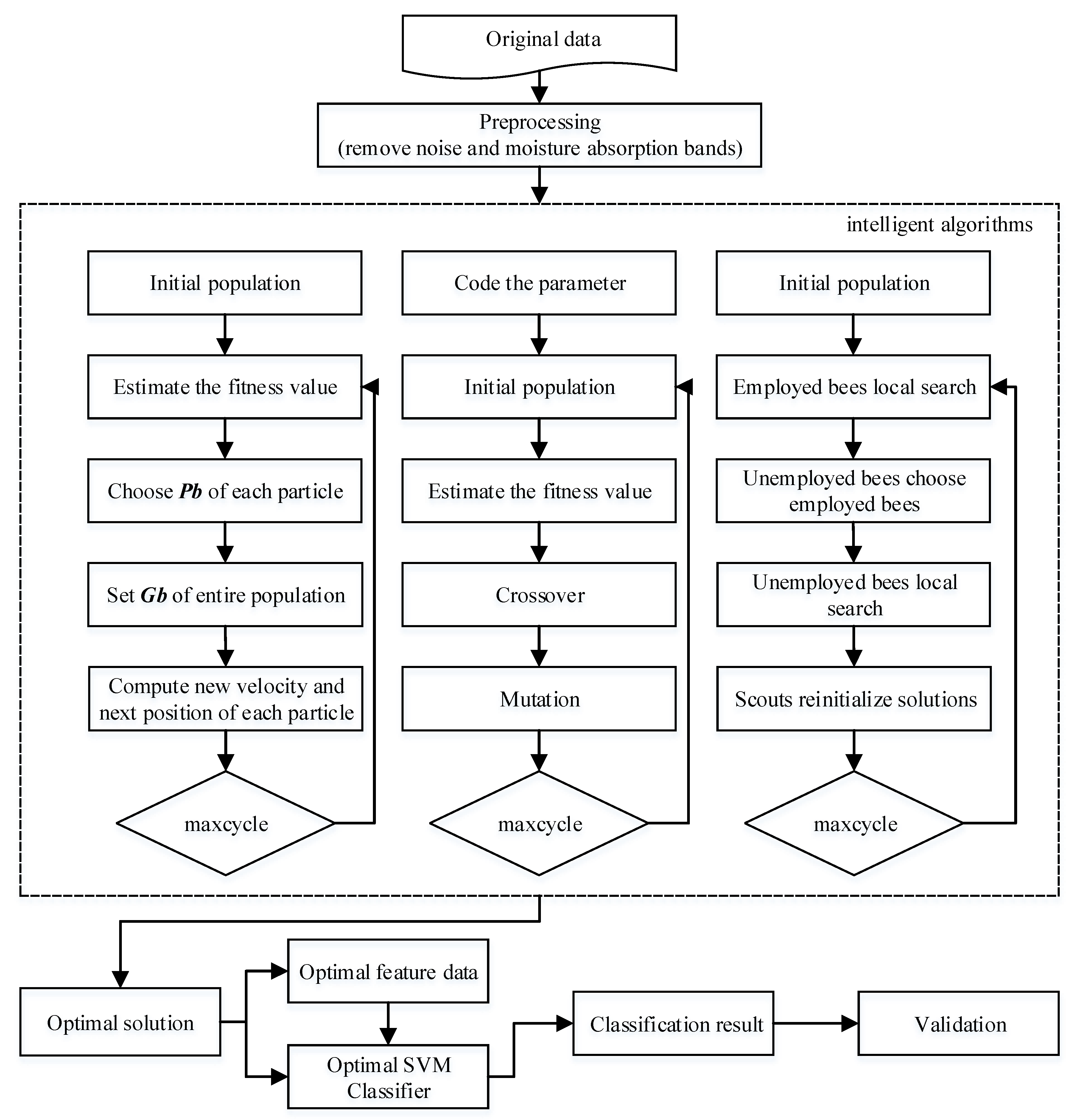
Karaboga [42] proposed the ABC algorithm in 2005. This swarm-intelligence optimization algorithm can be used to imitate the behavior of a bee colony searching for high quality nectar near the hive. In the ABC algorithm, the nectar is a potential solution in the hyperspace of the problem to be solved, and a fitness function measures the quality of the nectar, where the greater the fitness, the better the solution. The bee colony contains three types of bees: employed bees, unemployed bees, and scouts. The employed bees and unemployed bees will transform as scouts when the quantity of their nectars is low. The optimization process is based on two basic behavioral models of the colony (attracting bees to the solution with the highest fitness and abandoning the solution with lowest fitness). The procedure of the ABC algorithm is given, as follows.
Step 1. 
Randomly generate N e potential solutions for initialization in the D-dimensional hyperspace, S .
Step 2. 
Employed bees find new solutions, v , near their old solutions, x , according to v i j =   x i j + φ i j ( x i j x k j ) , where k { 1 , 2 , , N e } and k i , and k and j are generated randomly. The parameter v i j is the new value of the j-th parameter for the i-th employed bee. φ is a random number in the interval [−1,1], and v S .
Step 3. 
Each unemployed bee chooses an employed bee according to P ( x i ) = f i t ( x i ) m = 1 N e f i t ( x m ) , where P ( x i ) is the probability of the i-th employed bee being selected by the unemployed bees and f i t ( x m ) is the fitness of the m-th employed bee.
Step 4. 
If the solutions of the employed or unemployed bees are not optimized after l i m i t iterations, they will abandon their solutions and they’ll become scouts to generate new solutions (same as step 1). This procedure can make bee colony avoid falling into a local optimum.
Step 5. 
An iteration is terminated if the number of iteration reaches the pre-determined maximum number of iterations, MaxCycle. Otherwise, return to step two.

2.2. Genetic Algorithm

A GA is an intelligent algorithm that was proposed by Professor Holland in 1975 [43]. This method was inspired by Darwin’s biological evolution theory, and it searches for optimal solutions by simulating the natural selection mechanism of biological evolution in the real world. In GAs, the potential solution of the problem needs to be encoded as the chromosome that contains the parameters that needs to be optimized (the solution vector), and a parameter in a chromosome is called as a gene. The quality of chromosomes (potential solutions) is calculated through a fitness function. The chromosomes with higher fitness have higher probability to remain in the next generation. In the encoding process, the hyperspace is converted into a search space applicable to the genetic algorithm, and an initial population (a subset of potential solutions) is generated. Subsequently, the parents’ population generates offspring (a new generation of solutions) through crossover and mutation operations. In crossover, the parents’ chromosomes exchange some of their genes to generate new generation. After crossover, the genes of new generation may occasionally be altered in mutation. The crossover and mutation are the main operators of genetic algorithm, which can provide more alternate chromosomes (solutions) in successive populations. A selection operation is used to retain the solution with the highest fitness. Evolution from generation to generation then occurs, which allows for the algorithm to search for the optimal solution to the problem. The procedure of the GA is given, as follows.
Step 1. 
Code the parameters of the problem to be solved.
Step 2. 
Randomly generate the initial population, X ( 0 ) . Each chromosome represents a potential solution, whose dimension is D .
Step 3. 
Estimate the fitness value of each chromosome in the population according to a fitness function.
Step 4. 
Perform the genetic operations including crossover, mutations, selection etc.
Step 5. 
The iteration is terminated if the number of iteration reaches the pre-determined maximum number of iterations, MaxCycle. Otherwise, return to step two.

2.3. Particle Swarm Optimization

PSO is an evolutionary algorithm that was developed by scholars Kennedy et al. [44], which originated as a simulation of a bird flock, where each bird is considered as a “particle” (a potential solution). Each particle learns from its own and the other companion particles flying experience for finding the optimal solution. Each particle has three characteristics: velocity, position, and fitness (measurement quality). What is more, each particle has a memory of its previous best position. In the particle, the velocity determines the direction of a particle’s movement and the position is the current position (the combination of optimization parameters). A fitness function calculates the fitness, which represents the quality of the particle (solution). The higher the fitness, the better the particle. The core mechanisms of the particle swarm algorithm are velocity and position update. In Each iteration, the velocities of particles are updated in hyperspace according to experience of their own best position and the optimal particle (step 5). Subsequently, the positions of particles are adjusted according to the new velocities and its own previous positions (step 6). These two mechanisms mean that each move of particles is deeply influenced by its current position, its previous experience, and the knowledge of the whole swarm. Accordingly, after constant adjustment during the iterative process, the optimal solution is searched for in the hyperspace. The procedure of the PSO algorithm is given, as follows.
Step 1. 
Randomly generate an initial particle swarm of size N .
Step 2. 
Set the velocity vectors, v i , and position vectors, x i , of each particle ( i { 1 , 2 , , N } ), and measure the fitness of each particle in the population.
Step 3. 
Choose the best position of each particle that it experienced according to its fitness. ( P b i ,   i { 1 , 2 , , N } )
Step 4. 
Set the best position of entire swarm, G b according to the fitness function.
Step 5. 
Compute the new velocity of each particle, v i j t + 1 , with equation,   v i j t + 1 = v i j t + c 1 r a n d ( 0 , 1 ) ( P b i j t x i j t ) + c 2 r a n d ( 0 , 1 ) ( G b j t x i j t ) , j { 1 , , D } , c1 and c2 are positive random numbers between 0.0 and 1.0
Step 6. 
For each particle, move to the next position x i j t + 1 according to x i j t + 1 = x i j t + v i j t ,   j { 1 , , D } .
Step 7. 
The iteration is terminated if the number of iteration reaches the pre-determined maximum number of iterations, MaxCycle. Otherwise, go to step three.

2.4. SVM Optimized with the GI Algorithms

Because previous studies reported that a Gaussian kernel usually outperforms other kernels in SVM classifiers [23], in this study, we also used Gaussian kernels in our SVM. Figure 1 shows the classification of hyperspectral images with the SVM that was optimized with the GI algorithms. The optimization target of the three algorithms is to select the optimal parameters (C, σ) and feature subset. Therefore, a potential solution, X i , is the combination of the parameters of the SVM classifier and the selection probability in each band, as shown in Figure 1. The first two parameters represent the penalty parameter, C, and the SVM’s Radial Basis Function (RBF) kernel parameter, σ, where the range can be customized according to the data. The remaining parameters are the selection probability in each band, where nb represents the total number of bands in the data and b i is the selection probability of the i-th band, in the range [0,1]. We introduced a fitness function to measure the quality of the potential solutions:
f i t n e s s ( X i ) = ω · A c c + ( 1 ω ) · 1 i = 1 n b B i  
Equation (1) measures the fitness of the combination of selected bands and SVM optimization parameters, where ω is a weight in the range [0,1], and B i is the i-th band mask. If b i ≤ 0.5, then we set B i = 0, i.e., the i-th band is removed; otherwise, B i = 1, and the i-th band is preserved. Acc is calculated by using the three-fold cross-validation accuracy of the training samples to avoid over-fitting [45]. Here, to better understand, we take 5% of the training samples as an example to explain our method for calculating Acc. Firstly, we randomly selected 5% of the pixels from the origin hyperspectral data as training samples and the remaining 95% as validation samples. The training samples were used to calculate Acc. The validation samples were used to validate the classification accuracy of SVM that was optimized by GI algorithms. The training samples and validation samples are independent. Secondly, we further divided the training dataset (5% of the whole dataset) into three subsets (subset1, subset2, and subset3) and each subset was selected as the testing set in sequence with the remaining two subsets comprising the new training set. Thus, the training and testing samples are also independent during each classification testing process. The accuracy of each testing subset was calculated and Acc was the average accuracy of three tests. Actually, we compared the three, five, and 10-fold cross-validation accuracy of the training samples and found that the classification accuracy is, overall, not sensitive to the number of fold of cross validation (results are not shown in this paper). Therefore, in order to balance the computational load, we finally chose the three-fold cross validation. From Equation (1), the classification accuracy will be improved and fewer bands will be selected for better fitness.
Once the form of X i and f i t n e s s are set, ABC (GA, PSO)-SVM classification can be obtained by following the steps in Section 2.1, Section 2.2 and Section 2.3. The SVM classification process that was based on the three optimization algorithms is shown in Figure 2.

3. Data and Experiments

3.1. Data

Our tests were performed on three hyperspectral images: the University of Pavia image, Indian Pines image, and Salinas image, which represent the city, complicated farmland, and simple farmland, respectively. The images were downloaded from Purdue University’s MultiSpec website (ftp://ftp.ecn.purdue.edu/biehl/MultiSpec/) and their details are as follows.

3.1.1. University of Pavia Image

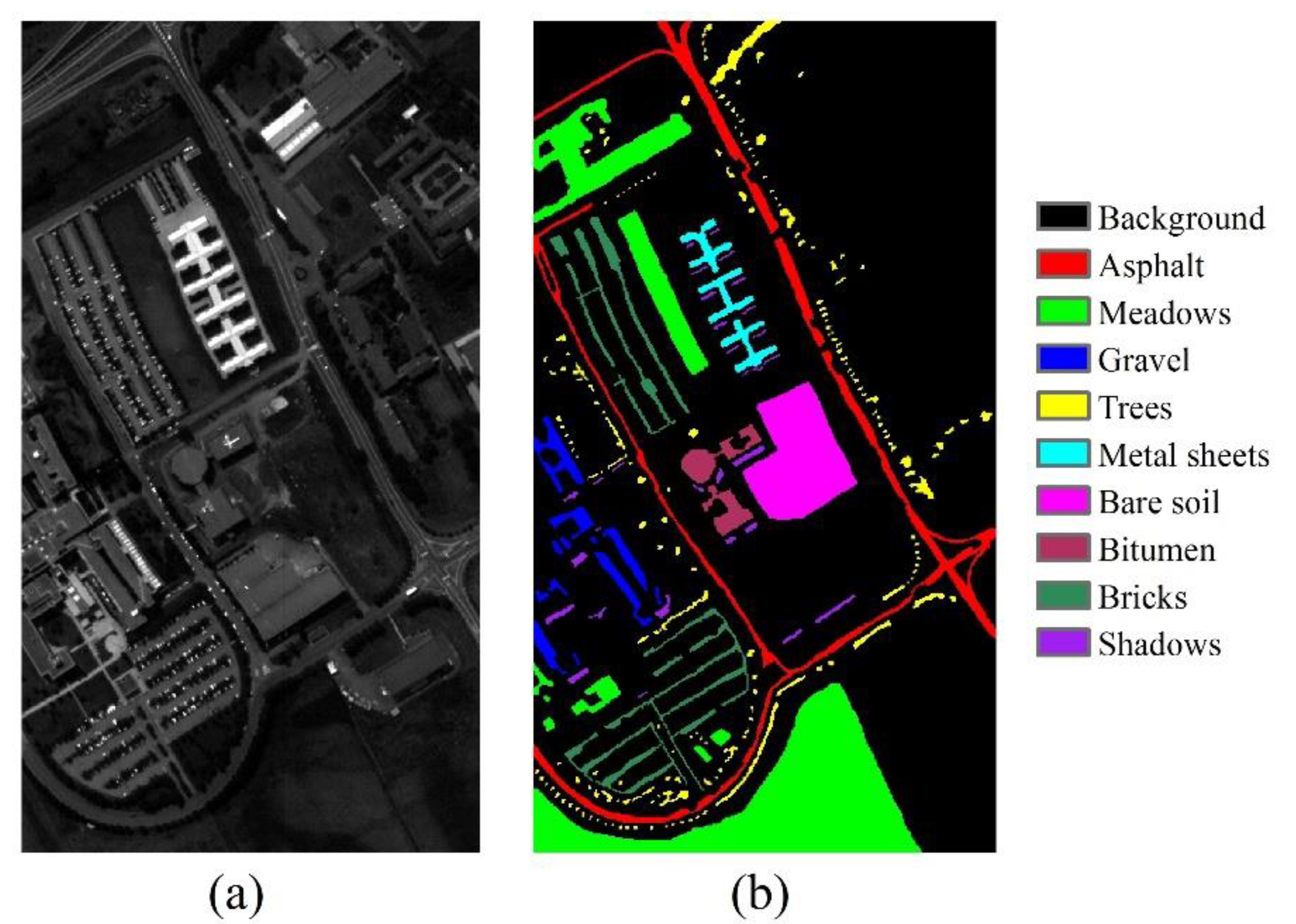
The University of Pavia image was acquired by the ROSIS sensor over Pavia, northern Italy. The image included 103 bands with 610 × 340 pixels at 1.3 m spatial resolution per pixel. The ground truth image contained nine classes. Figure 3 shows a color composite image of the University of Pavia and the corresponding ground truth data.

3.1.2. Indian Pines Image

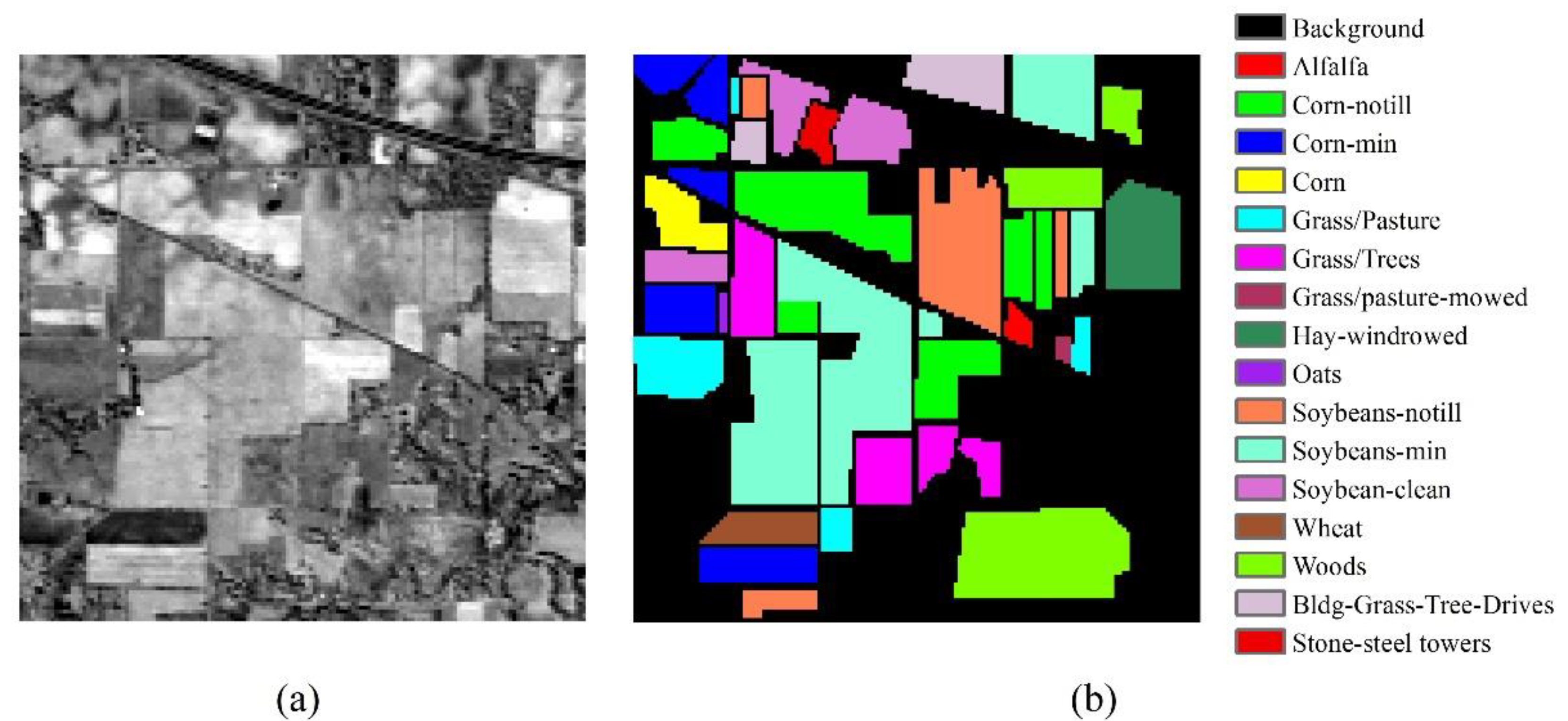
The AVIRIS Indian Pines dataset are comprised of a hyperspectral image that was obtained with the Airborne Visible/Infrared Imaging Spectrometer (AVIRIS) and a ground truth image. The AVIRIS Indian Pines image was acquired on 12 June 1992 over the northern part of Indiana, USA. After removing noise and moisture absorption bands (104–108, 150–163, 220) during preprocessing, the final dataset were comprised of 145 × 145 pixels and 200 bands. Figure 4a shows the optimized linear stretch of a sample band of the AVIRIS Indian Pines image and Figure 4b shows the ground truth image, which includes 16 classes in the study area.

3.1.3. Salinas Image

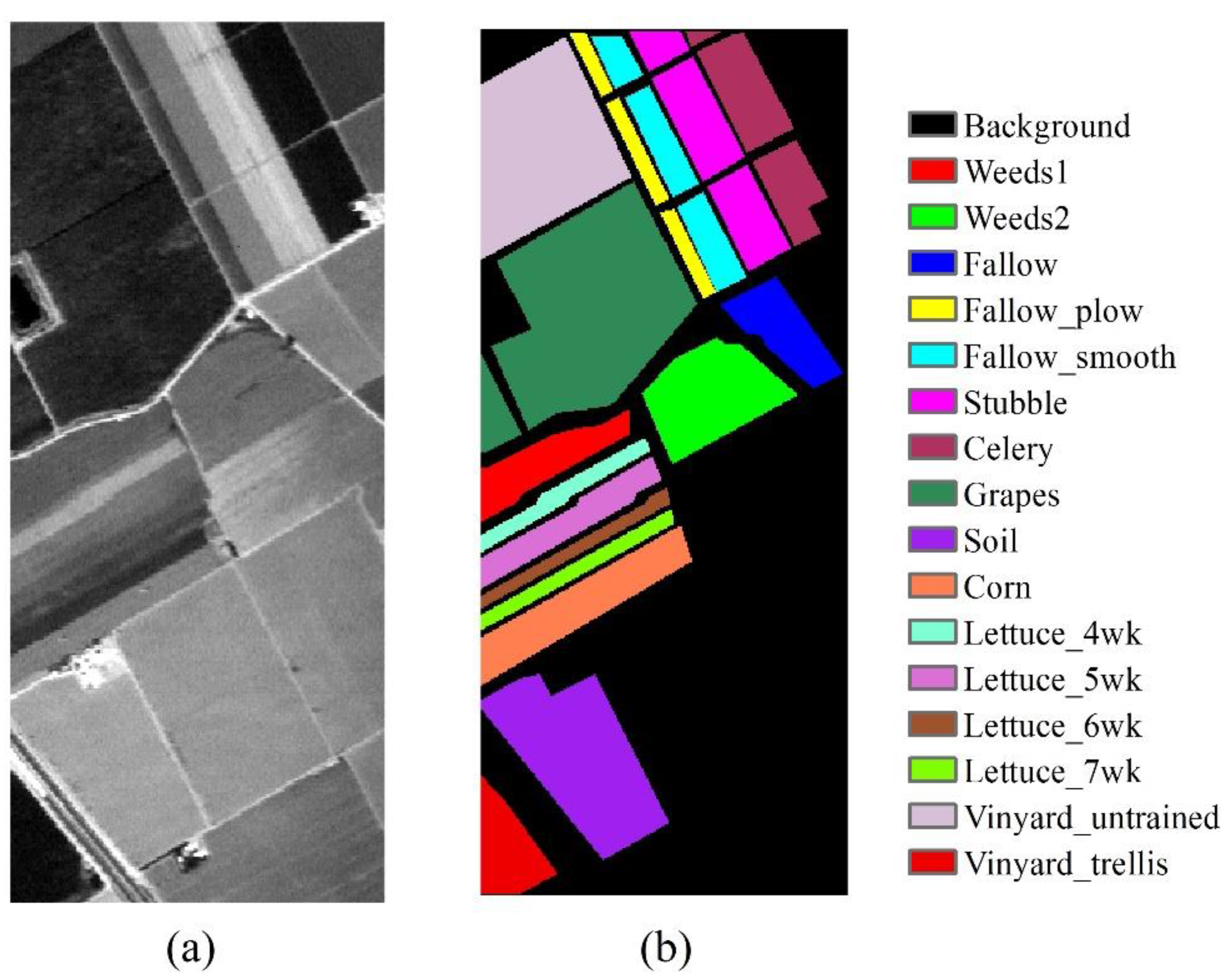
The Salinas image was obtained with the AVIRIS sensor over the Salinas Valley, California. The viewed area is comprised of 512 lines × 217 samples. The image includes 224 band and we removed 20 water absorption bands (108–112, 154–167, 224). The scene was only available as “at-sensor” radiance data and the ground truth image contained 16 classes. Figure 5 shows a sample band and ground truth images.

3.2. Experiment Design

To assess the impact of the training data size on the different GI algorithms, we separately applied the ABC-SVM, GA-SVM, and PSO-SVM pixel-wise classifiers to classify the pre-processed hyperspectral images while using training samples of varying sizes. Specifically, the three GI algorithms were trained using 5%, 10%, 15%, 20%, and 25% of the pixels from the overall dataset. We set the range of 0–25% sample size and the interval of 5% for of two reasons. Firstly, in practical applications, the number of high-quality training samples is often insufficient. Previous studies have pointed out that one advantage of SVM algorithm is to solve the problem of small sample size [46], which is also a reason why the SVM classifier is so popular. Therefore, the influence of sample size on classification algorithm is concerned with the difference of small sample size, not the difference of large sample size. A maximum sample rate is 20% in the reference [11] and 30% in the reference [47]. In comprehensive reference to above research [11,47], we set a maximum sample size of 25% of the original data set in this study. Secondly, an excessive sampling interval may lead to the loss of detailed accuracy change information. On the one hand, too small sampling interval will increase the computational complexity, on the other hand, the difference of accuracy may be very small. At the sampling interval of 0–25%, we eventually chose a 5% sampling interval to balance the computational complexity and the possible classification accuracy.
Stratified random sampling by class was used to collect independent training data sets. In each sample interval, an equal-sample-rate sampling method was used to randomly select a fixed percentage of pixels from each class as training samples. Each training set of a given size was used to train a classification ten times in order to avoid extreme situation. For each classification operation, we set the ranges of C, σ, and the band selection probability to [1,150], [0.1,1000], and [0,1], respectively. The computer that was employed had an i7-4790 processor running 64-bit Windows 10, and the proposed method was implemented in Matlab 2015b. The SVM was based on libSVM [48]. The parameters C and σ, the number of bands that were selected to participate in the classification (NB), the number of iterations (NI) were recorded. The overall accuracy (OA) of each classification was estimated in terms of the ground truth image and the mean, median, and standard deviation of OA were calculated. We then made comparisons of C, σ, NI, NB, and OA among ABC-SVM, GA-SVM, and PSO-SVM by using a variance analysis.

4. Results

4.1. Classification Results of the Three Hyperspectral Remote Sensing Datasets

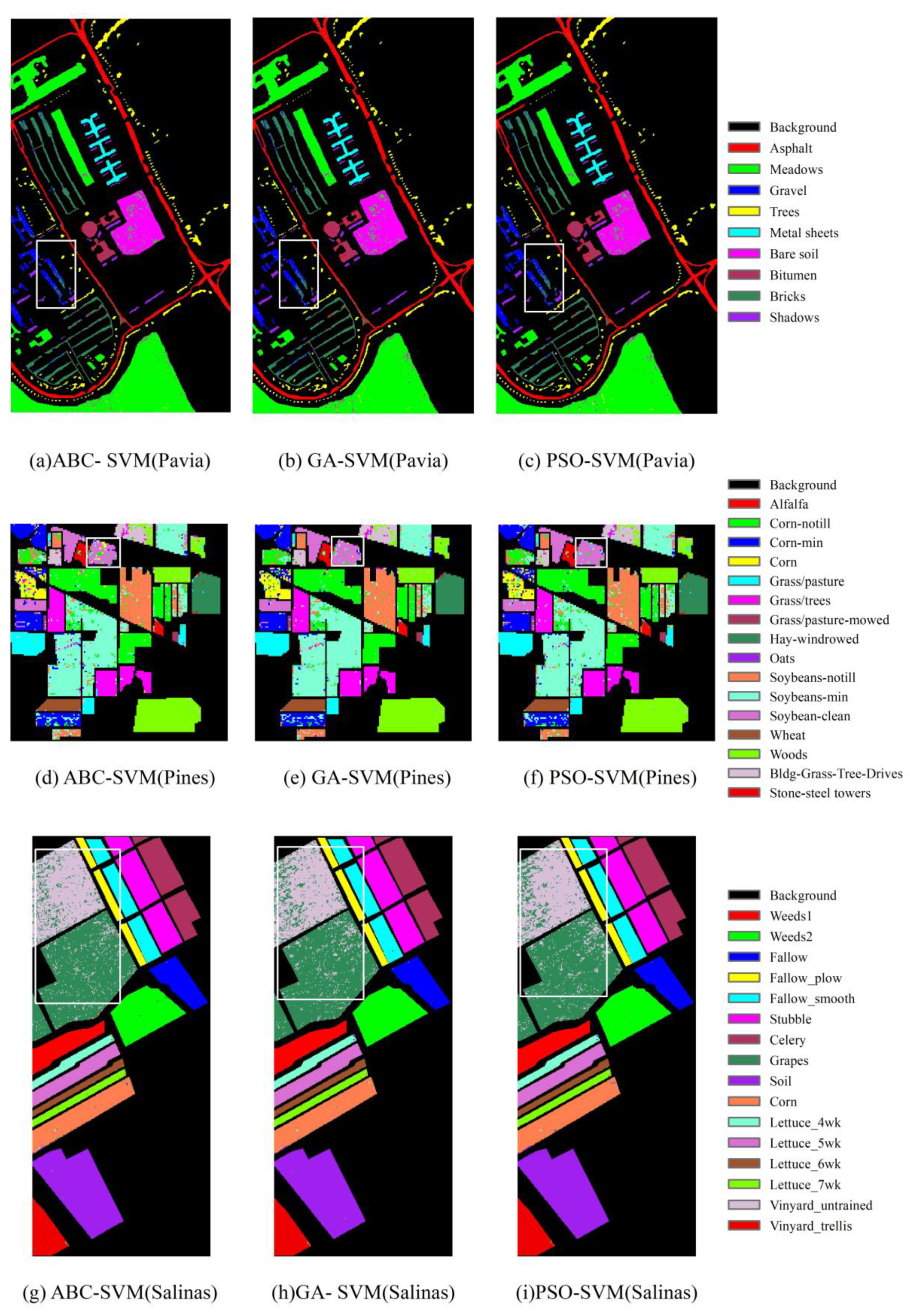
Table 1, Table 2 and Table 3 summarize the mean and standard deviation of the parameters C, σ, NI, NB, and OA of the SVM classifier that was optimized with three GI algorithms for different sample sizes (ranging from 5% to 25%, with 5% intervals). Figure 6 shows classification maps of the three hyperspectral remote sensing images when using the SVM classifier that was optimized with the three GI algorithms for a sample size of 25%.
For Pavia University, the dataset provided in Table 1, and for the same training sample dataset, the parameters C and σ optimized by the three GI algorithms were different. Moreover, for a given optimization algorithm, the parameters C and σ that were obtained by the 10 classification experiments were also different. As a whole, the standard deviation (SD) of the two parameters that were obtained from the PSO optimization is the lowest, while the SDs of the C(σ) parameters are 50.01 (14.06) and 11.27 (0.68) lower than those that were obtained with the ABC algorithm and the GA, respectively. The average NI used by the PSO algorithm is the smallest (15.54 and 33.28 smaller than those that were used by the ABC algorithm and the GA, respectively), and the average NB used by the GA is the smallest (25.32 and 30.92 lower than the ABC and PSO algorithms, respectively). The accuracies of the three algorithms are all quite similar. The PSO algorithm has the highest average accuracy, followed by the GA and the ABC algorithm. The PSO algorithm is 0.83% and 1.07% higher than the GA and ABC algorithm, respectively. Gravel has the most serious misclassification among the various types of objects. Some of the “Gravel” pixels are wrongly classified as “Bricks” (shown in rectangular boxes in the classification maps of Figure 6a–c). Misclassifications also occurred for “Bare Soil” in the center of the image and “Meadows” in the lower part of the classification maps.
Next, for the Indian Pines dataset (Table 2), similar to the Pavia University dataset, the parameters C and σ of the three GI algorithms are different for the same training sample dataset, and they also differ in the 10 classification experiments for a given fixed size training sample dataset and optimization algorithm. The order of NI of the three algorithms from high to low is GA (93.34), ABC (55.48), and PSO (43.88); while the order of NB from high to low is ABC (95.36), PSO (84.54), and GA (55.00). Unlike the Pavia University dataset, the SDs of the two parameters that were obtained by the PSO algorithm are the highest. The average OA of the three algorithms is obviously different, where in order from high to low is GA, AB, and PSO. It is found that GA is 8.23% and 16.43% more accurate than the ABC and PSO algorithms, respectively. The OA of the three optimization algorithms on the Indian Pines dataset is significantly lower than that on the other two datasets. The classification maps (Figure 6d–f) show considerable salt-and-pepper noise. The rectangular box on the map indicates the most obvious difference between the three algorithms. The commission errors of Soybean-clean is more serious in ABC-SVM than in the other two algorithms, in which more Soybean-clean pixels are wrongly identified as ‘Corn’ or ‘Corn-notill’.
Finally, the Salinas dataset (Table 3) was similar to the Pavia University and Indian Pines datasets, where the parameters C and σ of the three GI algorithms are different for the same training sample dataset, and they also differ in the 10 classifications experiments for a given fixed size training sample dataset and a given optimization algorithm. The NI and NB values from the PSO and ABC algorithms are close, and they both greatly differ with that obtained with the GA. The order of NI values from high to low is GA (93.48), ABC (56.78), and PSO (54.80); while the NB values from high to low are PSO (106.14), ABC (99.92), and GA (49.74). In terms of classification accuracy, similar to the Pavia University dataset, the accuracies of the three classification algorithms are not obviously different, which from high to low are PSO (94.40%), GA (94.17%), and ABC (93.50%). “Grapes” and “Vinyard_untrained” are the most easily confused among the different kinds of ground objects (as shown in the rectangular boxes in Figure 6g–i).

4.2. GI Algorithm Performance Comparison

For the three datasets, the homogeneity-of-variance tests were performed on the optimized parameters C and σ of the three GI algorithms, the number of bands selected, the number of iterations, and the classification accuracy (the results of different sample sizes are analyzed together in a given GI algorithm, therefore N = 50). If the variance was homogeneous, we performed a one-way ANOVA analysis and least significant difference (LSD) post hoc multiple comparisons (N = 150) while using the classification method as the factor, and C, σ, NI, NB, and OA as the dependents. Otherwise, we performed Welch’ ANOVA analysis and Games-Howell post hoc multiple comparisons.
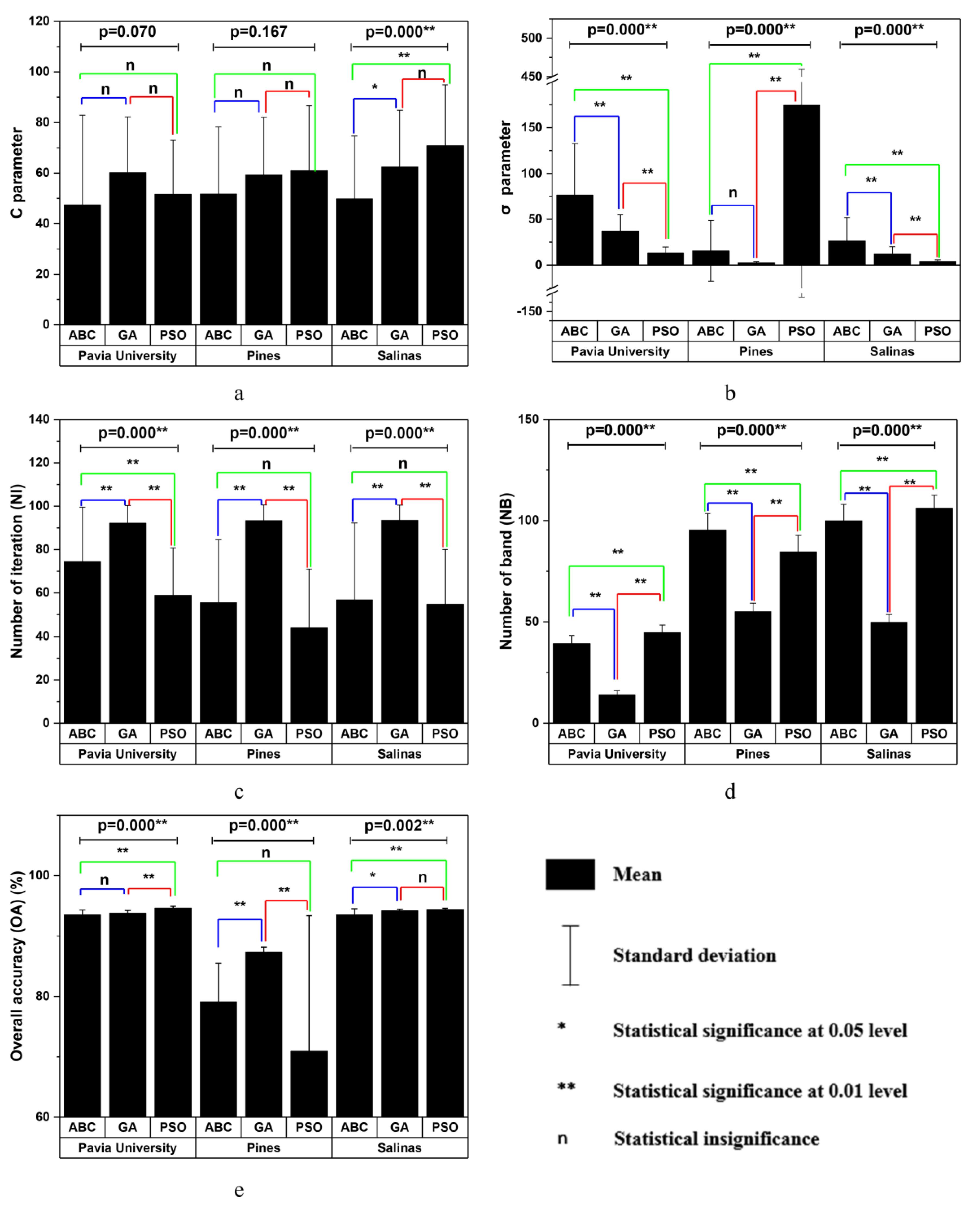
Figure 7 shows the difference between the optimization results of the different classification methods. There was no statistically significant difference (at the p = 0.05 level) in the C parameters between the Pavia University and the Indian Pines data, but there was a statistically significant difference in the Salinas data. The LSD comparisons show that the C parameters optimized with the ABC algorithm for the Salinas data are significantly different from those that were optimized by the PSO and GA algorithms at the p = 0.01 and p = 0.05 levels, respectively (Figure 7a).
The σ parameters obtained by the three optimization algorithms are significantly different (at the p = 0.01 level). The σ parameters obtained by PSO are significantly larger than those obtained from the ABC and GA optimizations (see Table 1, Table 2 and Table 3, and Figure 7b). The larger the σ parameters are, the easier it is to be over-fitted, which results in a reduction of classification accuracy.
The NIs of the three optimization algorithms were significantly different (at the p = 0.01 level). Overall, the number of iterations that were used by the GA was greater than that of the ABC and PSO algorithms (Figure 7c). The average numbers of iterations taken by the GA, ABC, and PSO algorithms in the 150 classification experiments of the three datasets were 93, 62, and 53, respectively.
The NB values that were selected by the three optimization algorithms were significantly different (at the p = 0.01 level). Generally, the number of bands selected by the algorithms was GA < PSO < ABC (Figure 7d). The average numbers of bands that were selected by the GA, PSO, and ABC algorithms in the 150 classification experiments on the three datasets were 40, 78, and 79, respectively. For the three datasets, the compression rates of between the ABC, GA, and PSO algorithms are 38–49%, 14–28%, and 42–52%, respectively; so, the GA has the strongest band compression ability.
The accuracy of the three optimization algorithms was also significantly different (at the p = 0.01 level). Overall, the GA had the highest average OA (91.77%), while the ABC algorithm had the second largest (88.73%), and the PSO algorithm had the lowest (86.65%) in all classification experiments. The classification accuracies of the three optimization algorithms for the Indian Pines dataset are obviously lower than those that were obtained for the other two datasets. The overall classification accuracy for the Pavia University, Indian Pines, and Salinas datasets was 94.00%, 79.12%, and 94.02% on average.

4.3. The Impact of Sample Size on GI Algorithms’ Performance

We carried out homogeneity-of-variance tests on parameters C and σ, NI, NB, and OA for the three kinds of GI algorithms and different sample sizes. If the variance was homogeneous, then we further performed a one-way ANOVA analysis (N = 50) using the sample size as the factor, and C, σ, NI, NB, and OA as the dependents. Otherwise, we performed Welch’s ANOVA analysis (N = 50). Figure 8 shows the effect of sample size on the optimization of each GI algorithm. Generally speaking, the sample size has no significant effect on the parameters C, NI and NB (Figure 8a,c,d). When the three hyperspectral datasets were classified by GA-SVM for the different sample sizes, the difference of the optimized parameters σ passed the test at the p = 0.01 significance level (Figure 8b); that is, when the parameters were optimized by the GA, the sample sizes had significant impact on the results of the σ parameter optimization. For the Salinas data, the σ parameters that were obtained by the three GI algorithms were significantly different at the p = 0.01 level. There is no significant difference in the classification accuracy of the Indian Pines dataset by PSO-SVM for the different sample sizes. However, the difference in the accuracy of other datasets that were classified by the three GI algorithms for different sample sizes all passed the significance test at the p = 0.01 level, which shows that the sample sizes generally have significant influence on the classification accuracy of the three GI algorithms.
In addition, for a given optimization algorithm, the classification accuracy increased with an increase of sample size (Figure 8e). For the three datasets, the classification accuracy of the Indian Pines dataset was significantly lower than that of the other two datasets (the significance of OA difference passed the p = 0.01 level test, which is not shown in Figure 8). In summary, the sample size has little effect on the feature selection, convergence speed, and parameter C of the GI algorithms, but it does have a significant effect on the final classification accuracy. The influence of sample size on parameter σ varies among the different datasets and different GI algorithms.

5. Discussion

The performances of the three optimization algorithms (GA, ABC, PSO) on the different datasets are different. For example, for the Salinas dataset, the OAs of the GA and the PSO methods are not significantly different. For the Pavia University dataset, the OAs of the ABC and GA methods are not significantly different. For the Indian Pines dataset, the OAs of the ABC and PSO methods are not significantly different (Figure 7e). The average OAs of these three datasets are 94.02%, 94.00%, and 79.12%, respectively, and the average classification accuracy of the Indian Pines datasets was about 15% lower than that of the other two images (Table 1, Table 2 and Table 3). This may be because the band dimension of the Indian Pines data is the highest. There are 16 land types in the Indian Pines data, which are mainly agricultural land. The land types of Indian Pines are more complex and confusing than those of Salinas and Pavia University. For the Indian Pines dataset, the GA had the highest classification accuracy (the average classification accuracy was 87.34%, 8.23% higher than the ABC algorithm, and 16.42% higher than the PSO algorithm) and the best stability (the SD of the classification accuracy was 0.82%, which was 5.54% lower than that obtained with the ABC algorithm, and 21.63% lower than that obtained with the PSO algorithm; see Table 2). In addition, from the analysis that is given in Section 4, we can see that the data compression ability of the GA algorithm is the strongest among the three optimization algorithms, where its compression capacity is more than 70%. It has been pointed out that the number of bands in the considered hyperspectral images affects the classification accuracies of SVMs. Selecting the appropriate feature bands before classifying hyperspectral images is helpful in addressing the problem of dimensionality disaster and improving the classification accuracy [17]. Therefore, the GA algorithm is preferred for hyperspectral image classification, especially for complex research scenes. The classification accuracy for the same sample size is also related to the quality of the sample [11,14], the spectral separability of the target objects [49,50], and the number of characteristic bands that are involved in the classification [17].
Sample size has a significant impact on the optimization results of the three optimization algorithms. On the whole, the larger the sample size, the higher the average classification accuracy. In contrast, there is no relationship between the stability of the classification accuracy and the sample size (for example, for the Indian Pines dataset, PSO-SVM has a greater change in accuracy for different sample sizes, as shown in Figure 8e). Therefore, in the actual classification process, it is suggested to increase the number of samples, especially the number of effective samples. For SVM classification, valid samples are the support vector samples [14]. If the total number of samples increases, but the number of valid samples does not increase, then the classification accuracy might not be improved. Samples of support vectors are usually located at the edge of the spectral feature space of different classes, so the spectral feature space of the object type in the study area is analyzed before classification, and useful boundary samples for constructing the optimal segmentation hyperplane can be found to increase the number of effective samples [11]. In the case of a certain number of samples, when compared with multi-spectral remote sensing data, hyperspectral data has a high dimension and strong correlation between bands. It is easy to suggest that the classification accuracy is reduced due to insufficient sample size (e.g., the Hughes effect). This problem easily manifests in the case of small sample sizes. Reducing the number of feature bands [17] and improving the number of labeled samples by combining semi-supervised classification [51] can also improve the classification accuracy.
In our study, for the small sample sizes (e.g., 5% of the total sample size considered in this paper), the accuracy of the three classification methods is quite similar. The average classification accuracy of the ABC, GA, and PSO algorithms for the Pavia University dataset is 91.31%, 92.52%, and 92.99%, respectively, while the average classification accuracy of these GIs on the Salinas dataset is 91.67%, 93%, and 93.14%, respectively. For complex research scenes, the accuracy of the three classification methods greatly varies. The average classification accuracy of the ABC, GA, and PSO algorithms for the Indian Pines dataset is 65.72%, 81.90%, and 70.80%, respectively. With an increase of sample size, the accuracy increase of ABC-SVM is the most obvious. For example, when the sample size increased from 5% to 25%, the average classification accuracy of ABC-SVM improved by about 20% (65.72% to 85.95%), the average classification accuracy of GA-SVM improved by about 9% (81.90% to 90.78%), while the average classification accuracy of the SVM decreased by about 5% (70.80% to 65.89%). Therefore, while considering the influence of sample size on the optimization algorithm, the GA is recommended, especially in the case of small sample sizes.
For the SVM, C is the penalty coefficient, that is, the tolerance of error, where the higher the tolerance of error, the more likely over-fitting will occur; otherwise, the smaller C is, the more likely that under-fitting with occur. The smaller σ is, the larger the curvature of the decision boundary is, and the easier it is that over fitting happens, and vice versa. Similar decision boundaries can be obtained while using different combinations of C and σ [23]. In our study, the three optimization algorithms have less influence on the parameter C than on the parameter σ (Figure 7a,b and Figure 8a,b). Therefore, in this paper, the OA values are different when using the three GI algorithms to optimize the SVM when classifying a given hyperspectral image with the same training data; the difference may be more, because the three optimization algorithms have significant differences in the parameter σ optimization. The reason that the three optimization algorithms have less influence on the parameter C optimization that is done by the SVM than on the parameter σ may be that the interval of the parameter C in this paper is [1,150], which is smaller than the interval of the parameter σ [0.1,1000]. Therefore, improving the stability of classification accuracy and shortening the time of data processing by setting reasonable C and σ parameters intervals, and making the search intervals as small as possible, which allow the GI algorithms to more easily determine the optimal parameters is helpful [52]. Table 4 shows an example that verifies the effect of the initial range of σ on the optimization results of the three GI algorithms. In this example, we made a comparison test in which the training sample size and the range of C parameter were same, but the range of σ parameter was set to [0.1,300] and [300,600], respectively. Specifically, in all tests, the training sample size was 25% and the range of C parameter was set to [1,150]. Overall, the σ parameter with range of [0.1,300] has higher classification accuracy than the σ parameter with range of [300,600], especially for the Pine dataset.

6. Conclusions

In this paper, we used three GI algorithms (GA, and the PSO and ABC algorithms) to optimize a SVM and classify three hyperspectral images of the University of Pavia, Indian Pines, and Salinas while using training samples of varying sizes. Based on the classification results, we compared the optimization performance of the three GI algorithms on the SVM in five aspects: the stability to parameter settings, convergence rate, feature selection ability, sample size, and classification accuracy. Our results show:
(1) The influence of the three optimization algorithms on the C-parameter optimization of the SVM is less than that on the σ-parameter. The convergence rate, the significant difference, the number of selected features, and the accuracy of three GI algorithms are statistically significantly different (at the p = 0.01 level). The number of features that were selected by the ABC, GA, and PSO algorithms is 38–49%, 14–28%, and 42–52% of the original data bands, respectively. The GA has the strongest feature-selection ability, and it can compress more than 70% of the original data. In addition, the average overall accuracy of GA-SVM on three images was the highest (91.77%), followed by ABC-SVM (88.73%) and PSO-SVM (86.65%). Moreover, the classification accuracies of the three optimization algorithms for the Indian Pines datasets were significantly lower than those of the other two datasets.
(2) Sample size has a significant impact on the optimization results of the three optimization algorithms. Generally speaking, the larger the sample size, the higher the average classification accuracy. For small sample sizes (e.g., 5% of the total sample size considered in this paper), from the numerical point of view, the accuracies of the three classification methods for simple research area (University of Pavia and Salinas images) are similar; however, for complex scenes (Indian Pines Image), they are very different. Of the three optimization algorithms, the sample size has the greatest impact on the accuracy of the ABC-SVM optimization algorithm, followed by PSO-SVM and GA-SVM.
In summary, the data dimension, complexity of the study area, and sample size all affect the optimization performance of the three optimization algorithms. When compared with the ABC and PSO algorithms, the GA has more advantages in terms of feature band selection, small sample size classification, and classification accuracy.

Author Contributions

N.L. and X.Z. conceived of the study and designed the experiments; N.L. performed the experiments; Y.P. analyzed the data; N.L. and X.Z. wrote the paper.

Funding

This work was supported by the National Natural Science Foundation for Distinguished Young Scholars of China (Grant No. 41401479), Project Supported by State Key Laboratory of Earth Surface Processes and Resource Ecology (Grant No. 2017-FX-01(1)) and the Major Project of High-Resolution Earth Observation System. (Grant No. E03071112).

Conflicts of Interest

The authors declare no conflict of interest.

References

  1. Chapelle, O.; Vapnik, V.; Bousquet, O.; Mukherjee, S. Choosing multiple parameters for support vector machines. Mach. Learn. 2002, 46, 131–159. [Google Scholar] [CrossRef]
  2. Dalponte, M.; Bruzzone, L.; Gianelle, D. Fusion of hyperspectral and lidar remote sensing data for classification of complex forest areas. IEEE Trans. Geosci. Remote Sens. 2008, 46, 1416–1427. [Google Scholar] [CrossRef]
  3. Kuemmerle, T.; Chaskovskyy, O.; Knorn, J.; Radeloff, V.C.; Kruhlov, I.; Keeton, W.S.; Hostert, P. Forest cover change and illegal logging in the ukrainian carpathians in the transition period from 1988 to 2007. Remote Sens. Environ. 2009, 113, 1194–1207. [Google Scholar] [CrossRef]
  4. Fauvel, M.; Benediktsson, J.A.; Chanussot, J.; Sveinsson, J.R. Spectral and spatial classification of hyperspectral data using svms and morphological profiles. IEEE Trans. Geosci. Remote Sens. 2008, 46, 3804–3814. [Google Scholar] [CrossRef]
  5. Cao, X.; Chen, J.; Imura, H.; Higashi, O. A svm-based method to extract urban areas from dmsp-ols and spot vgt data. Remote Sens. Environ. 2009, 113, 2205–2209. [Google Scholar] [CrossRef]
  6. Ma, X.; Tong, X.; Liu, S.; Luo, X.; Xie, H.; Li, C. Optimized sample selection in svm classification by combining with dmsp-ols, landsat ndvi and globeland30 products for extracting urban built-up areas. Remote Sens. 2017, 9, 236. [Google Scholar] [CrossRef]
  7. Zhang, Y.; Wang, C.; Wu, J.; Qi, J.; Salas, W.A. Mapping paddy rice with multitemporal alos/palsar imagery in southeast china. Int. J. Remote Sens. 2009, 30, 6301–6315. [Google Scholar] [CrossRef]
  8. Löw, F.; Michel, U.; Dech, S.; Conrad, C. Impact of feature selection on the accuracy and spatial uncertainty of per-field crop classification using support vector machines. ISPRS J. Photogramm. Remote Sens. 2013, 85, 102–119. [Google Scholar] [CrossRef]
  9. Hurni, K.; Schneider, A.; Heinimann, A.; Nong, D.H.; Fox, J. Mapping the expansion of boom crops in mainland southeast asia using dense time stacks of landsat data. Remote Sens. 2017, 9, 320. [Google Scholar] [CrossRef]
  10. Han, X.; Chen, X.; Feng, L. Four decades of winter wetland changes in poyang lake based on landsat observations between 1973 and 2013. Remote Sens. Environ. 2015, 156, 426–437. [Google Scholar] [CrossRef]
  11. Foody, G.M.; Mathur, A.; Sanchez-Hernandez, C.; Boyd, D.S. Training set size requirements for the classification of a specific class. Remote Sens. Environ. 2006, 104, 1–14. [Google Scholar] [CrossRef]
  12. Huang, C.; Davis, L.S.; Townshend, J.R.G. An assessment of support vector machines for land cover classification. Int. J. Remote Sens. 2002, 23, 725–749. [Google Scholar] [CrossRef]
  13. Zhu, X.; Pan, Y.; Jinshui, Z.; Wang, S.; Gu, X.; Xu, C. The effects of training samples on the wheat planting area measure accuracy in tm scale(i): The accuracy response of different classifiers to training samples. J. Remote Sens. 2007, 11, 826–837. [Google Scholar] [CrossRef]
  14. Foody, G.M.; Mathur, A. Toward intelligent training of supervised image classifications: Directing training data acquisition for svm classification. Remote Sens. Environ. 2004, 93, 107–117. [Google Scholar] [CrossRef]
  15. Foody, G.M.; Mathur, A. The use of small training sets containing mixed pixels for accurate hard image classification: Training on mixed spectral responses for classification by a svm. Remote Sens. Environ. 2006, 103, 179–189. [Google Scholar] [CrossRef]
  16. Melgani, F.; Bruzzone, L. Classification of hyperspectral remote sensing images with support vector machines. IEEE Trans. Geosci. Remote Sens. 2004, 42, 1778–1790. [Google Scholar] [CrossRef] [Green Version]
  17. Pal, M.; Foody, G.M. Feature selection for classification of hyperspectral data by svm. IEEE Trans. Geosci. Remote Sens. 2010, 48, 2297–2307. [Google Scholar] [CrossRef]
  18. Pal, M.; Mather, P.M. Support vector machines for classification in remote sensing. Int. J. Remote Sens. 2005, 26, 1007–1011. [Google Scholar] [CrossRef]
  19. Inglada, J. Automatic recognition of man-made objects in high resolution optical remote sensing images by svm classification of geometric image features. ISPRS J. Photogramm. Remote Sens. 2007, 62, 236–248. [Google Scholar] [CrossRef]
  20. Dash, J.; Mathur, A.; Foody, G.M.; Curran, P.J.; Chipman, J.W.; Lillesand, T.M. Land cover classification using multi-temporal meris vegetation indices. Int. J. Remote Sens. 2007, 28, 1137–1159. [Google Scholar] [CrossRef]
  21. Waske, B.; Linden, S.v.d.; Benediktsson, J.A.; Rabe, A.; Hostert, P. Sensitivity of support vector machines to random feature selection in classification of hyperspectral data. IEEE Trans. Geosci. Remote Sens. 2010, 48, 2880–2889. [Google Scholar] [CrossRef]
  22. Foody, G.M. Rvm-based multi-class classification of remotely sensed data. Int. J. Remote Sens. 2008, 29, 1817–1823. [Google Scholar] [CrossRef]
  23. Ben-Hur, A.; Weston, J. A User’s Guide to Support Vector Machines. In Data Mining Techniques for the Life Sciences; Springer: New York, NY, USA, 2010; pp. 223–239. [Google Scholar]
  24. Cawley, G.C.; Talbot, N.L. On over-fitting in model selection and subsequent selection bias in performance evaluation. J. Mach. Learn. Res. 2010, 11, 2079–2107. [Google Scholar]
  25. Devos, O.; Ruckebusch, C.; Durand, A.; Duponchel, L.; Huvenne, J.-P. Support vector machines (svm) in near infrared (nir) spectroscopy: Focus on parameters optimization and model interpretation. Chemom. Intell. Lab. Syst. 2009, 96, 27–33. [Google Scholar] [CrossRef]
  26. Guo, B.; Gunn, S.R.; Damper, R.I.; Nelson, J.D.B. Customizing kernel functions for svm-based hyperspectral image classification. IEEE Trans. Image Process. 2008, 17, 622–629. [Google Scholar] [CrossRef] [PubMed]
  27. Tuia, D.; Camps-Valls, G.; Matasci, G.; Kanevski, M. Learning relevant image features with multiple-kernel classification. IEEE Trans. Geosci. Remote Sens. 2010, 48, 3780–3791. [Google Scholar] [CrossRef]
  28. Samadzadegan, F.; Hasani, H.; Schenk, T. Simultaneous feature selection and svm parameter determination in classification of hyperspectral imagery using ant colony optimization. Can. J. Remote Sens. 2012, 38, 139–156. [Google Scholar] [CrossRef]
  29. Bazi, Y.; Melgani, F. Toward an optimal svm classification system for hyperspectral remote sensing images. IEEE Trans. Geosci. Remote Sens. 2006, 44, 3374–3385. [Google Scholar] [CrossRef]
  30. Liu, X.; Li, X.; Peng, X.; Li, H.; He, J. Swarm intelligence for classification of remote sensing data. Sci. China Ser. D Earth Sci. 2008, 51, 79–87. [Google Scholar] [CrossRef]
  31. Li, N.; Zhu, X.; Pan, Y.; Zhan, P. Optimized svm based on artificial bee colony algorithm for remote sensing image classification. J. Remote Sens. 2018, 22, 559–569. [Google Scholar] [CrossRef]
  32. Jayanth, J.; Ashok Kumar, T.; Koliwad, S.; Krishnashastry, S. Identification of land cover changes in the coastal area of dakshina kannada district, south india during the year 2004–2008. Egypt. J. Remote Sens. Space Sci. 2016, 19, 73–93. [Google Scholar] [CrossRef]
  33. Xue, Z.; Du, P.; Su, H. Harmonic analysis for hyperspectral image classification integrated with pso optimized svm. IEEE J. Sel. Top. Appl. Earth Obs. Remote Sens. 2014, 7, 2131–2146. [Google Scholar] [CrossRef]
  34. Kuo, R.-J.; Huang, S.L.; Zulvia, F.E.; Liao, T.W. Artificial bee colony-based support vector machines with feature selection and parameter optimization for rule extraction. Knowl. Inf. Syst. 2018, 55, 253–274. [Google Scholar] [CrossRef]
  35. Hughes, G. On the mean accuracy of statistical pattern recognizers. IEEE Trans. Inf. Theory 1968, 14, 55–63. [Google Scholar] [CrossRef]
  36. Pal, M. Support vector machine-based feature selection for land cover classification: A case study with dais hyperspectral data. Int. J. Remote Sens. 2006, 27, 2877–2894. [Google Scholar] [CrossRef]
  37. Bradley, P.E.; Keller, S.; Weinmann, M. Unsupervised feature selection based on ultrametricity and sparse training data: A case study for the classification of high-dimensional hyperspectral data. Remote Sens. 2018, 10, 1564. [Google Scholar] [CrossRef]
  38. Li, S.; Wu, H.; Wan, D.; Zhu, J. An effective feature selection method for hyperspectral image classification based on genetic algorithm and support vector machine. Knowl. Based Syst. 2011, 24, 40–48. [Google Scholar] [CrossRef]
  39. Ghamisi, P.; Benediktsson, J.A. Feature selection based on hybridization of genetic algorithm and particle swarm optimization. IEEE Geosci. Remote Sens. Lett. 2015, 12, 309–313. [Google Scholar] [CrossRef]
  40. Sukawattanavijit, C.; Chen, J.; Zhang, H. Ga-svm algorithm for improving land-cover classification using sar and optical remote sensing data. IEEE Geosci. Remote Sens. Lett. 2017, 14, 284–288. [Google Scholar] [CrossRef]
  41. Wang, M.; Wan, Y.; Ye, Z.; Lai, X. Remote sensing image classification based on the optimal support vector machine and modified binary coded ant colony optimization algorithm. Inf. Sci. 2017, 402, 50–68. [Google Scholar] [CrossRef]
  42. Karaboga, D. An Idea Based on Honey Bee Swarm for Numerical Optimization. Technical Report-tr06; Erciyes University, Engineering Faculty, Computer Engineering Department: Kayseri, Turkey, 2005. [Google Scholar]
  43. Holland, J.H. Adaptation in Natural and Artificial Systems: An Introductory Analysis with Applications to Biology, Control, and Artificial Intelligence; MIT Press: Cambridge, MA, USA, 1992. [Google Scholar]
  44. Eberhart, R.; Kennedy, J. A New Optimizer Using Particle Swarm Theory. In MHS’95, Proceedings of the Sixth International Symposium on Micro Machine and Human Science, Nagoya, Japan, 4–6 October 1995; IEEE: Piscataway, NJ, USA, 1995; pp. 39–43. [Google Scholar]
  45. Stone, M. Cross-validatory choice and assessment of statistical predictions. J. R. Stat. Society Ser. B (Methodol.) 1974, 36, 111–147. [Google Scholar] [CrossRef]
  46. Mountrakis, G.; Im, J.; Ogole, C. Support vector machines in remote sensing: A review. ISPRS J. Photogramm. Remote Sens. 2011, 66, 247–259. [Google Scholar] [CrossRef]
  47. Camps-Valls, G.; Tuia, D.; Bruzzone, L.; Benediktsson, J.A. Advances in hyperspectral image classification: Earth monitoring with statistical learning methods. IEEE Signal Process. Mag. 2014, 31, 45–54. [Google Scholar] [CrossRef]
  48. Chang, C.-C.; Lin, C.-J. Libsvm: A library for support vector machines. Acm Trans. Intell. Syst. Technol. 2011, 2, 1–27. [Google Scholar] [CrossRef]
  49. Samsudin, S.H.; Shafri, H.Z.; Hamedianfar, A.; Mansor, S. Spectral feature selection and classification of roofing materials using field spectroscopy data. J. Appl. Remote Sens. 2015, 9, 095079. [Google Scholar] [CrossRef]
  50. Tamimi, E.; Ebadi, H.; Kiani, A. Evaluation of different metaheuristic optimization algorithms in feature selection and parameter determination in svm classification. Arab. J. Geosci. 2017, 10, 478. [Google Scholar] [CrossRef]
  51. Ghoggali, N.; Melgani, F. Genetic svm approach to semisupervised multitemporal classification. IEEE Geosci. Remote Sens. Lett. 2008, 5, 212–216. [Google Scholar] [CrossRef]
  52. Silva, R.; Gomes, V.; Mendes-Faia, A.; Melo-Pinto, P. Using support vector regression and hyperspectral imaging for the prediction of oenological parameters on different vintages and varieties of wine grape berries. Remote Sens. 2018, 10, 312. [Google Scholar] [CrossRef]
Figure 1. Support vector machine (SVM) optimization parameters.
Remotesensing 11 00734 g001
Figure 2. SVM classification process based on the three optimization algorithms.
Remotesensing 11 00734 g002
Figure 3. University of Pavia (a) sample band (band 10) and (b) ground truth image.
Remotesensing 11 00734 g003
Figure 4. Airborne Visible/Infrared Imaging Spectrometer (AVIRIS) Indian Pines (a) sample band (band 100), and (b) ground truth image.
Remotesensing 11 00734 g004
Figure 5. Salinas (a) sample band (band 5) and (b) ground truth image.
Remotesensing 11 00734 g005
Figure 6. Classification maps of the Pavia University (ac), Indian Pines (df), and Salinas (gi) images.
Remotesensing 11 00734 g006
Figure 7. Comparison of three group intelligence (GI) algorithms optimization on the SVM in five aspects: (a) C parameter, (b) σ parameter, (c) number of iteration, (d) number of band and (e) overall accuracy.
Remotesensing 11 00734 g007
Figure 8. The impact of sample size on each GI algorithm’s performance including (a) C parameter, (b) σ parameter, (c) number of iteration, (d) number of band and (e) overall accuracy. (1, 2, 3, 4, and 5 refer to sampling ratios of 5%, 10%, 15%, 20%, and 25%, respectively)
Remotesensing 11 00734 g008
Table 1. Classification parameters and performance of the Pavia University image.
MethodParameters/PerformanceSample SizeMean
5%10%15%20%25%
ABCCMean49.2034.6751.6544.7657.1147.48
SD38.9132.3028.2228.6648.9535.41
σMean78.4468.7747.0992.8994.6176.36
SD65.7557.1039.7360.5358.5356.33
Number of iterations (NI)Mean63.0082.8079.8081.5065.0074.42
SD38.4920.3121.5121.9523.3525.12
Number of band (NB)Mean40.9040.1040.7037.8037.1039.32
SD4.614.823.064.083.383.99
overall accuracy (OA)Mean91.31%93.05%94.21%94.32%94.94%93.56%
SD1.151.010.670.830.380.81
GACMean77.6153.7454.4468.0247.2060.20
SD16.8918.9127.2516.9430.1622.03
σMean17.7639.3437.2351.2340.5037.21
SD10.2410.8122.0126.6718.2117.59
Number of iterations (NI)Mean92.6091.5090.8093.7092.2092.16
SD7.887.319.377.538.708.16
Number of band (NB)Mean15.4013.6014.1013.6013.3014.00
SD2.631.652.771.511.832.08
overall accuracy (OA)Mean92.52%93.51%94.00%94.39%94.57%93.80%
SD0.560.400.420.400.440.45
PSOCMean59.1250.3656.9143.7847.8751.61
SD25.6923.7121.3920.6615.2721.35
σMean9.1411.6913.1318.2314.7313.38
SD7.356.344.1310.932.866.32
Number of iterations (NI)Mean57.2067.7061.7047.8060.0058.88
SD22.5319.5324.8720.4721.7621.83
Number of band (NB)Mean45.2046.9046.4043.2042.9044.92
SD4.613.573.503.332.423.49
overall accuracy (OA)Mean92.99%94.35%95.12%95.37%95.34%94.63%
SD0.410.240.190.250.390.30
Table 2. Classification parameters and performance of the Indian Pines image.
MethodParameters/PerformanceSample SizeMean
5%10%15%20%25%
ABCCMean59.5535.2660.1342.6060.8451.68
SD23.2930.4823.2225.0430.7826.56
σMean51.317.796.985.715.2015.40
SD139.178.605.646.406.4633.25
Number of iterations (NI)Mean55.3055.7053.2066.1047.1055.48
SD38.7532.3524.4321.1628.6329.06
Number of band (NB)Mean95.6097.5097.3093.2093.2095.36
SD11.883.549.738.836.718.14
overall accuracy (OA)Mean65.72%77.06%81.79%85.04%85.95%79.11%
SD15.417.133.853.052.396.36
GACMean69.9049.9065.9465.4145.2559.28
SD15.4120.6321.2031.6724.9922.78
σMean1.112.942.271.833.742.38
SD0.622.161.220.543.281.56
Number of iterations (NI)Mean93.4091.5095.1092.6094.1093.34
SD10.397.854.516.836.547.23
Number of band (NB)Mean59.4056.0055.8052.4051.4055.00
SD2.504.855.693.954.064.21
overall accuracy (OA)Mean81.90%85.09%88.80%90.12%90.78%87.34%
SD0.801.700.570.640.410.82
PSOCMean60.7162.3666.1963.6451.8760.95
SD27.9629.1221.4519.0530.8525.68
σMean66.47187.83169.36111.20337.33174.44
SD209.37317.16272.96233.01393.60285.22
Number of iterations (NI)Mean57.4041.4045.2040.9034.5043.88
SD33.0224.4530.5323.7623.8127.11
Number of band (NB)Mean84.0084.6087.4084.6082.1084.54
SD7.697.598.557.699.368.18
overall accuracy (OA)Mean70.80%68.04%71.16%78.71%65.89%70.92%
SD16.9225.3024.8220.9124.2722.45
Table 3. Classification parameters and performance of the Salinas image.
MethodParameters/PerformanceSample SizeMean
5%10%15%20%25%
ABCCMean46.4856.0361.2447.4837.8249.81
SD31.8323.5223.9326.3518.5824.84
σMean13.1622.836.1343.1346.3926.33
SD12.2819.746.0651.2038.7725.61
Number of iterations (NI)Mean53.5055.7058.0049.9066.8056.78
SD33.4940.5031.7239.5332.1035.47
Number of band (NB)Mean101.7099.6099.50100.1098.7099.92
SD7.2910.658.497.256.938.12
overall accuracy (OA)Mean91.67%93.14%93.32%94.16%95.21%93.50%
SD1.06%0.98%1.39%1.19%0.47%1.02%
GACMean69.0662.0572.6043.9464.1962.37
SD11.0226.1727.0527.6820.3722.46
σMean4.5510.4110.6220.2513.9011.95
SD1.675.225.3417.0311.128.07
Number of iterations (NI)Mean97.4092.2095.1088.6094.1093.48
SD2.329.595.2210.557.427.02
Number of band (NB)Mean52.9049.0049.4048.2049.2049.74
SD3.903.923.172.825.533.87
overall accuracy (OA)Mean93.00%93.92%94.35%94.60%94.98%94.17%
SD0.24%0.34%0.22%0.30%0.28%0.28%
PSOCMean59.4483.9273.9969.8766.9270.83
SD29.8412.3723.6326.1728.3624.07
σMean2.282.484.085.865.614.06
SD0.880.531.192.742.561.58
Number of iterations (NI)Mean54.0050.6053.4060.3055.7054.80
SD26.2025.6817.7528.6727.8425.23
Number of bands (NB)Mean108.50106.00109.20105.80101.20106.14
SD8.296.226.295.276.146.44
overall accuracy (OA)Mean93.14%94.11%94.65%94.89%95.23%94.40%
SD0.23%0.12%0.23%0.20%0.22%0.20%
Table 4. The overall accuracy of three GI algorithms with different σ range setting.
DatasetsABCGAPSO
[0.1,300][300,600][0.1,300][300,600][0.1,300][300,600]
Pavia University95.31%91.02%94.17%95.31%95.31%94.79%
Pine89.43%42.89%91.29%53.57%89.22%42.89%
Salinas94.95%87.35%94.90%94.22%95.37%90.58%