Optimized Contrast Enhancement for Infrared Images Based on Global and Local Histogram Specification

Abstract

In this paper, an optimized contrast enhancement method combining global and local enhancement results is proposed to improve the visual quality of infrared images. Global and local contrast enhancement methods have their merits and demerits, respectively. The proposed method utilizes the complementary characteristics of these two methods to achieve noticeable contrast enhancement without artifacts. In our proposed method, the 2D histogram, which contains both global and local gray level distribution characteristics of the original image, is computed first. Then, based on the 2D histogram, the global and local enhanced results are obtained by applying histogram specification globally and locally. Lastly, the enhanced result is computed by solving an optimization equation subjected to global and local constraints. The pixel-wise regularization parameters for the optimization equation are adaptively determined based on the edge information of the original image. Thus, the proposed method is able to enhance the local contrast while preserving the naturalness of the original image. Qualitative and quantitative evaluation results demonstrate that the proposed method outperforms the block-based methods for improving the visual quality of infrared images.

1. Introduction

Recent years, infrared imaging systems have been extensively applied in military and civilian areas such as night version, video surveillance, driver assistance, fire detection, and disease diagnosis [1,2,3]. In these areas, infrared imaging has broad application prospects due to its ability to reflect the thermal radiation distribution of the scene, which is impossible for visual imaging. However, compared with visual images, there are many inherent drawbacks in infrared images. Among these drawbacks, the low contrast and low resolution are the key factors that reduce the visual quality of infrared images [4]. Therefore, contrast enhancement is essential for improving the visual quality of infrared images.

Contrast enhancement methods have been studied for decades, and they can be categorized into two families depending on the area adopted for defining the enhancement method such as global contrast enhancement (GCE) and local contrast enhancement (LCE) [5]. The GCE methods aim to enhance the overall contrast by finding a mapping function and considering the characteristics of the entire image. On the contrary, LCE methods try to enhance the local contrast of each area by using different mapping functions, which are correlated to the characteristics of the local areas.

As for the GCE methods, histogram equalization (HE) [6] is one of the most well-known methods. Due to the low computational complexity and effective contrast enhancement capability, HE has been widely applied to improve the visual quality of images. However, the enhanced results of HE may cause serious over-enhancement artifacts when there are large, homogeneous regions in infrared images [7]. To deal with this problem, some improved HE methods have been investigated. Among these methods, the plateau histogram equalization (PHE) [8,9], double plateaus histogram equalization (DPHE) [10], and adaptive double plateaus histogram equalization (ADPHE) [11] try to introduce one or two proper thresholds to avoid over-enhancement. Besides these plateau-based methods, some other methods such as the brightness preserving bi-histogram equalization (BBHE) [12], dualistic sub-image histogram equalization (DSIHE) [13], recursive mean-separate histogram equalization (RMSHE) [14], adaptive histogram segmentation (AHS) [15], and adaptive histogram partition (AHP) [16] address the over-enhancement by adaptively dividing the histogram into two or more partitions. Other methods such as the histogram modification framework (HMF) [17] and histogram specification (HS) [18] also gives better performance for avoiding over-enhancement. In summary, the GCE methods aim to make a trade-off between avoiding over-enhancement and enhancing the contrast as much as possible [15]. Although the GCE methods naturally improve the contrast with low computational complexity and good light order preservation, the single mapping function ignores the local contrast characteristics of the image, which limits the performance of GCE methods.

The LCE methods try to enhance the local contrast by taking the characteristics of local areas into consideration. One effective approach is to divide the input image into multiple sub-blocks and then enhance the contrast of each sub-block respectively. For instance, this includes the contrast limited adaptively histogram equalization (CLAHE) [19] and partially overlapped sub-block histogram equalization (POSHE) [20]. The CLAHE method divides the input image into multiple non-overlapped sub-blocks and the histogram of each sub-block is clipped and redistributed to limit the contrast. The bilinear interpolation is also introduced to prevent the blocking artifacts. The POSHE method prevents the blocking artifacts by dividing the input image into a partially overlapped sub-block and the enhanced results of the pixels in overlapped areas are computed based on the correlated sub-blocks. By improving the CLAHE method with a new redistribution mechanism and local contrast enhancement, the balanced CLAHE and contrast enhancement (BCCE) [21] performs better than CLAHE in terms of visual quality improvement. The adaptive trilateral contrast enhancement (ATCE) [22] utilizes the double plateau histogram equalization for the local contrast enhancement and then manipulates the sharpness and intensity based on the extracted feature of the input image. Nevertheless, these methods may still suffer from blocking artifacts and over-enhancement in homogeneous regions. In order to take the content of each sub-block into consideration, the mechanisms for calculating the mapping functions of the sub-blocks can vary along with the local content. Thus, the adjacent-blocks-based modification for local histogram equalization (ABMHE) [23] and local gradient-grayscale statistical feature (LGGSF) [24] categorize the sub-blocks into two or three categories. For each category, the particular mechanism is applied to calculate the mapping functions of the sub-blocks. Besides these block-based methods, other LCE methods called unsharp masking (UM) based methods [25,26,27,28,29] decompose the input image into a base layer and a detail layer by a filter. These two layers are enhanced separately and then composited to get the final enhanced image. Some other methods introduce the retinex theory [30,31] and the wavelet transform [32,33] to realize the contrast enhancement of infrared images. The LCE methods have better performance for improving the local contrast, but they may cause unnatural and over-enhanced results in some local areas.

As described above, the GCE and LCE methods have complementary characteristics. It is necessary to study a new contrast enhancement method that combines the metrics of both methods [5,34]. These methods are designed for the visual color images while there are no color components and the contrast is poor in the infrared images. Therefore, they are not suitable for the infrared images. In this paper, based on the 2D histogram, an optimized contrast enhancement method combining the merits of global and local methods is proposed to improve the visual quality of infrared images. First, the 2D histogram, which contains both global and local gray level distribution characteristics of the input image, is computed according to the definition in Reference [35]. Then, based on the histogram specification, the global and local contrast enhancement are conducted. The global mapping function is obtained by applying a histogram specification to the clipped and redistributed 2D histogram. The local mapping functions are also computed by applying histogram specification to each row of the 2D histogram and then updated based on the global mapping function. The GCE and LCE results are computed based on the global mapping function and local mapping functions. Lastly, an objective function is conducted with global and local constrained conditions and the optimized enhancement result is obtained through the optimization approach. Thus, the final enhanced image is possible to make a compromise between the merits of global and local enhancements. The main contributions of our paper are: (1) The 2D histogram is utilized to realize both global and local contrast enhancement. (2) The global enhancement result is obtained by applying the histogram specification to the clipped 2D histogram. (3) The local mapping functions are computed by applying the histogram specification to each row of the 2D histogram. The local enhancement result is obtained based on the local content information and the corresponding mapping functions. (4) The desired image is obtained by finding a solution for the quadratic optimization function, which contains both global and local constrained conditions. For the local content adaptation, the edge information of the input image is also taken into consideration.

The remainder of this paper is organized as follows. In Section 2, we first make a brief review of the 2D histogram. In Section 3, we describe the proposed method in detail. Section 4 gives the experimental results and Section 5 concludes the paper.

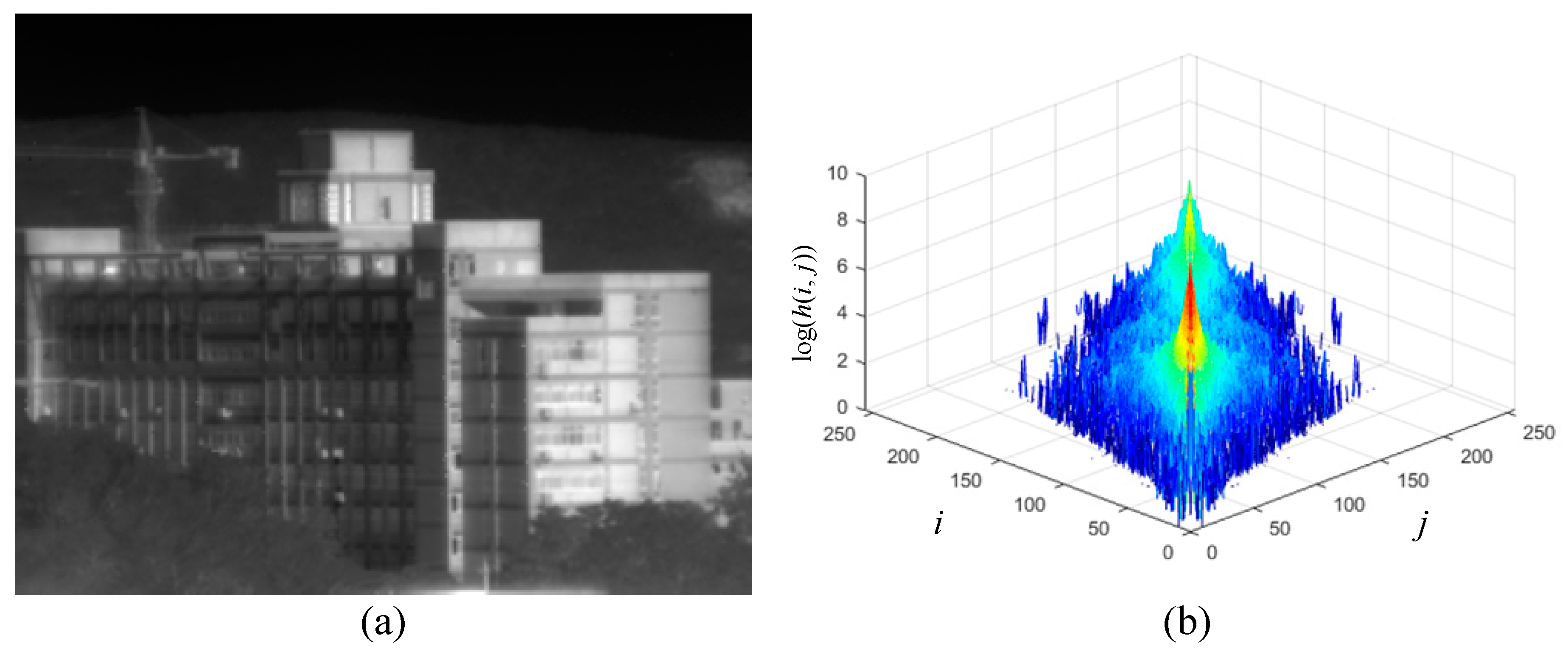
2. Review of the 2D Histogram

The concept of the 2D histogram was first proposed in Reference [35] to improve the contrast of visual images. In that paper, the 2D histogram $h(i,j)$ was defined to indicate the joint distribution of two spatially adjacent pixels with grey levels $i$ and $j$, respectively. For a given input image $X$ of size $M\times N$ pixels and dynamic range $\left[x_d,x_u\right]$, i.e., $X=\left\{x(m,n)|1\le m\le M,1\le n\le N,x(m,n)\in \mathbb{N}\right\}$ and $x(m,n)\in [x_d,x_u]$. The main objective of the contrast enhancement methods is to generate an enhanced image $Y$ of the same size as $X$, i.e., $Y=\left\{y(m,n)|1\le m\le M,1\le n\le N,y(m,n)\in \mathbb{N}\right\}$, which has better visual quality than $X$ and $y(m,n)\in [y_d,y_u]$. The dynamic range of $Y$ can be stretched or compressed [35]. For an 8-bit image, the dynamic range of the enhanced image is $\left[0,255\right]$ to take full use of the entire dynamic range. For the input image, assume that the dynamic range is $\left[0,L-1\right]$, and $L=256$ for the 8-bit image, which is the number of distinct gray-levels of the image. The 2D histogram can be expressed as the equation below.

$$H=\left\{h(i,j)|\text{}0\le i\le L-1,0\le j\le L-1\right\}$$

(1)

where $h(i,j)$ is the number of the occurrences of gray level $j$ in the neighborhood of gray level $i$ and $h(i,j)$ is computed as the equation below.

$$h(i,j)={\displaystyle \sum _{m=1}^M{\displaystyle \sum _{n=1}^N{\displaystyle \sum _{k=-r}^r{\displaystyle \sum _{l=-r}^r{\varphi }_{i,j}(x(m,n),x(m+k,n+l))}}}}$$

(2)

where $r$ is an integer introduced to determine the square $(2r+1)\times (2r+1)$ neighborhood around each pixel. The binary function ${\varphi }_{i,j}(u,v)$ is used to identify the occurrence of the gray levels $i$ and $j$ at the spatial square neighborhood and is defined as the equation below.

$${\varphi }_{i,j}(u,v)=\{\begin{array}{l}\begin{array}{cc}1,& ifu=iandv=j\end{array}\\ \begin{array}{cc}0,& otherwise\end{array}\end{array}$$

(3)

In order to apply the 2D histogram to the calculation of global mapping function, the 2D histogram is redefined in Reference [36] as follows.

$$h(i,j)={\displaystyle \sum _{m=1}^M{\displaystyle \sum _{n=1}^N{\displaystyle \sum _{k=-r}^r{\displaystyle \sum _{l=-r}^r{\varphi }_{i,j}(x(m,n),x(m+k,n+l))(\left|i-j\right|+1)}}}}$$

(4)

In this scenario, the initial 2D histogram is weighted by the absolute-valued differences $\left(\left|i-j\right|+1\right)$. Therefore, higher weight is assigned to the 2D histogram when the difference between $i$ and $j$ is large. The 2D histogram based global contrast enhancement method gets better performance for improving the visual quality of visual images. However, due to the low contrast of infrared images, the global contrast enhancement is not enough for the visual quality improvement of infrared images.

3. Proposed Method

In this section, the proposed method is described in detail, which includes histogram specification-based global and local contrast enhancement and the optimized enhancement result combining both global and local enhanced results. The 2D histogram is utilized in our proposed method to achieve both global and local contrast enhancement. Figure 1 shows the overall block diagram of the proposed method.

Usually, the data width of the raw images captured by an infrared imaging system is 14-bit and the histogram of the raw image is sparse. This means that most of the gray levels take on no pixel. Therefore, we pre-process the raw images by removing the gray levels that take no pixel and linearly mapping the remaining ordered gray levels to $\left[0,2^8-1\right]$. In order to obtain both global and local enhancement results based on the 2D histogram, the 2D histogram should contain both global and local gray level distribution characteristics of the input image. Thus, in our proposed method, the 2D histogram is calculated based on the definition in Equation (2).

Take an infrared image for reference. Figure 2 shows the reference infrared image and its normalized 2D histogram using a $5\times 5$ neighborhood. There are more dark regions than bright regions. Therefore, the 2D histogram has larger values located at lower gray values. There are also some homogeneous regions in the image. The neighbors of each pixel in these homogeneous regions take on very similar gray levels, which result in higher peaks at the diagonal or near-diagonal element of the 2D histogram. As can be observed in Figure 2b, the 2D histogram is diagonal symmetry. This is due to the mutual relation between each pixel and its neighbors.

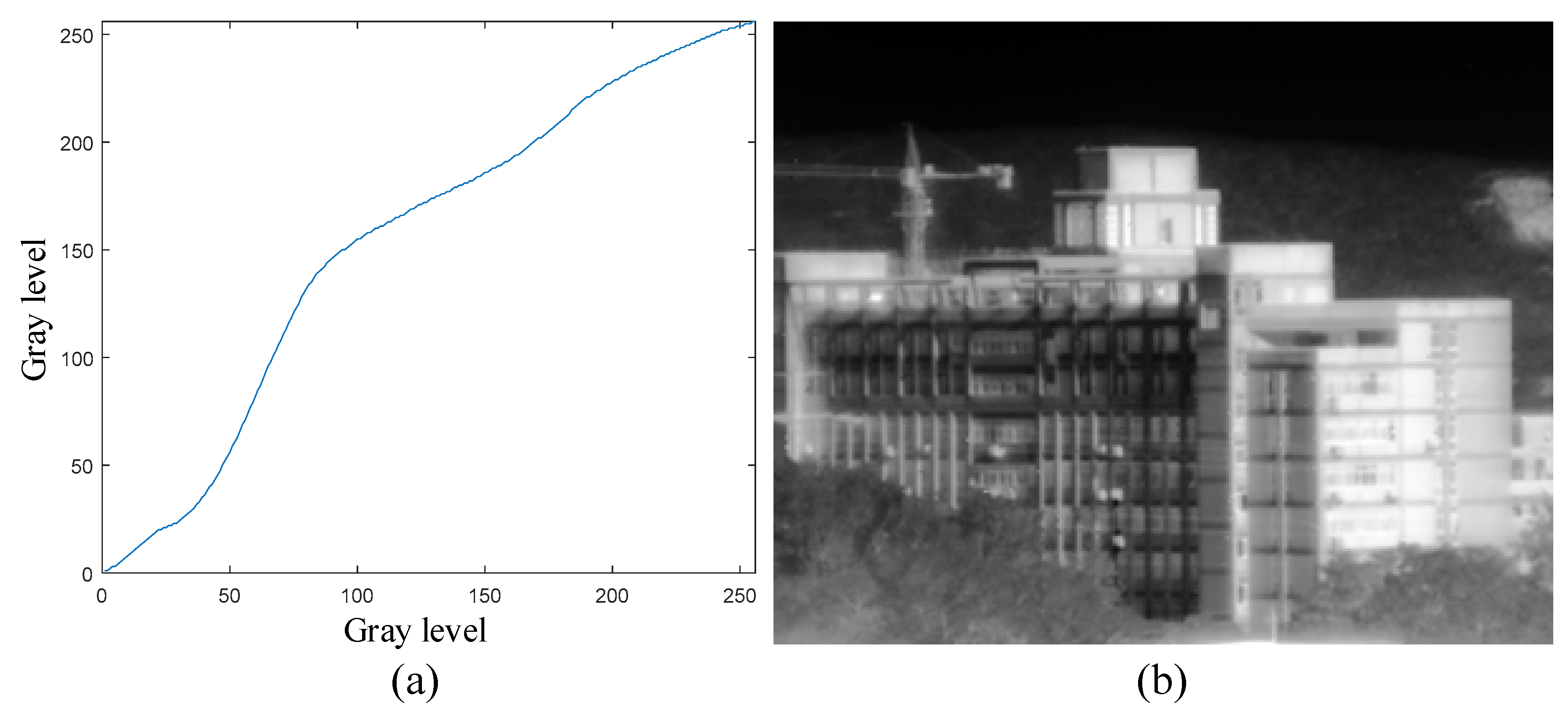
3.1. Global Enhancement

Global enhancement methods aim to obtain an optimized mapping function to map the input image to an enhanced one for better visual quality. In order to obtain the mapping function, the histogram specification is utilized in this case. First of all, to improve the global contrast and avoid over-enhancement, the 2D histogram is clipped by an adaptively adjusted clip point [37] as shown below.

$$h^{\ast }(i,j)=\{\begin{array}{ll}h(i,j)& h(i,j)\le clip\\ clip& h(i,j)>clip\end{array}$$

(5)

where the $clip$ is computed by the formula below.

$$clip=\frac{MN{(2r+1)}^2}{L^2}(1+\frac{\beta }{100}{H}^{\max })$$

In this case, $H^{\max }$ is the maximum value of the 2D histogram while $\beta$ is the clipping factor and is set to be 0.2 for the experiments in this paper. The exceeded pixels are then equally redistributed and the updated 2D histogram $H^{\ast }=\left\{h^{\ast }(i,j)|0\le i\le L-1,0\le j\le L-1\right\}$ is normalized according to the equation below.

$$h^{\ast }(i,j)=h^{\ast }(i,j)/{\displaystyle \sum _{i^{\prime }=0}^{L-1}{\displaystyle \sum _{j^{\prime }=0}^{L-1}{h}^{\ast }(i,j)}}$$

(6)

Based on the modified 2D histogram, the corresponding cumulative distribution function is written as the equation below.

$$C_G=\left\{c_G(i)={\displaystyle \sum _{k=0}^i{\displaystyle \sum _{j=0}^{L-1}{h}^{\ast }(k,j)}}|i=0,1,\cdots ,L-1\right\}$$

(7)

Then, as for the desired 2D histogram, it is supposed to satisfy the following uniformly distributed probability density function [36].

$$\widehat{H}=\left\{\widehat{h}(i^{\prime },j^{\prime })=\frac{1}{L^2}|0\le i^{\prime }\le L-1,0\le j^{\prime }\le L-1\right\}$$

(8)

Similarly, the corresponding cumulative distribution function of the desired 2D histogram is computed as the equation below.

$${\widehat{C}}_G=\left\{{\widehat{c}}_G(i^{\prime })={\displaystyle \sum _{k=0}^{i^{\prime }}{\displaystyle \sum _{j=0}^{L-1}\widehat{h}(k,l)}}|i^{\prime }=0,1,\cdots ,L-1\right\}$$

(9)

Combining Equations (7) and (9), according to the definition of the histogram specification [38], the mapping function aims to map the gray level $i$ of the 2D histogram to the gray level $i^{\prime }$ of the desired 2D histogram and satisfy the equation $c_G(i)={\widehat{c}}_G(i^{\prime })$. Therefore, the mapping function is computed according to the equation below.

$$T_G=\left\{t_G(i)=\underset{i^{\prime }\in \{0,1,\cdots ,L-1\}}{\arg \min }\left|c_G(i)-{\widehat{c}}_G(i^{\prime })\right||i=0,1,\cdots ,L-1\right\}$$

(10)

Using Equation (10), the gray levels of the input image $X$ are transformed to the corresponding gray levels of the enhanced output image. Thus, the global enhancement result $Y_G$ is computed by the formula below.

$$Y_G=\left\{y_G(m,n)=t_G(x(m,n))|1\le m\le M,1\le n\le N\right\}$$

(11)

The resultant global mapping function and the enhanced image are shown in Figure 3a,b. As observed in Figure 3b, the global enhanced result gets a natural appearance and improves the contrast without any artifacts. However, there is no improvement in terms of local contrast. Therefore, the enhancement performance is limited.

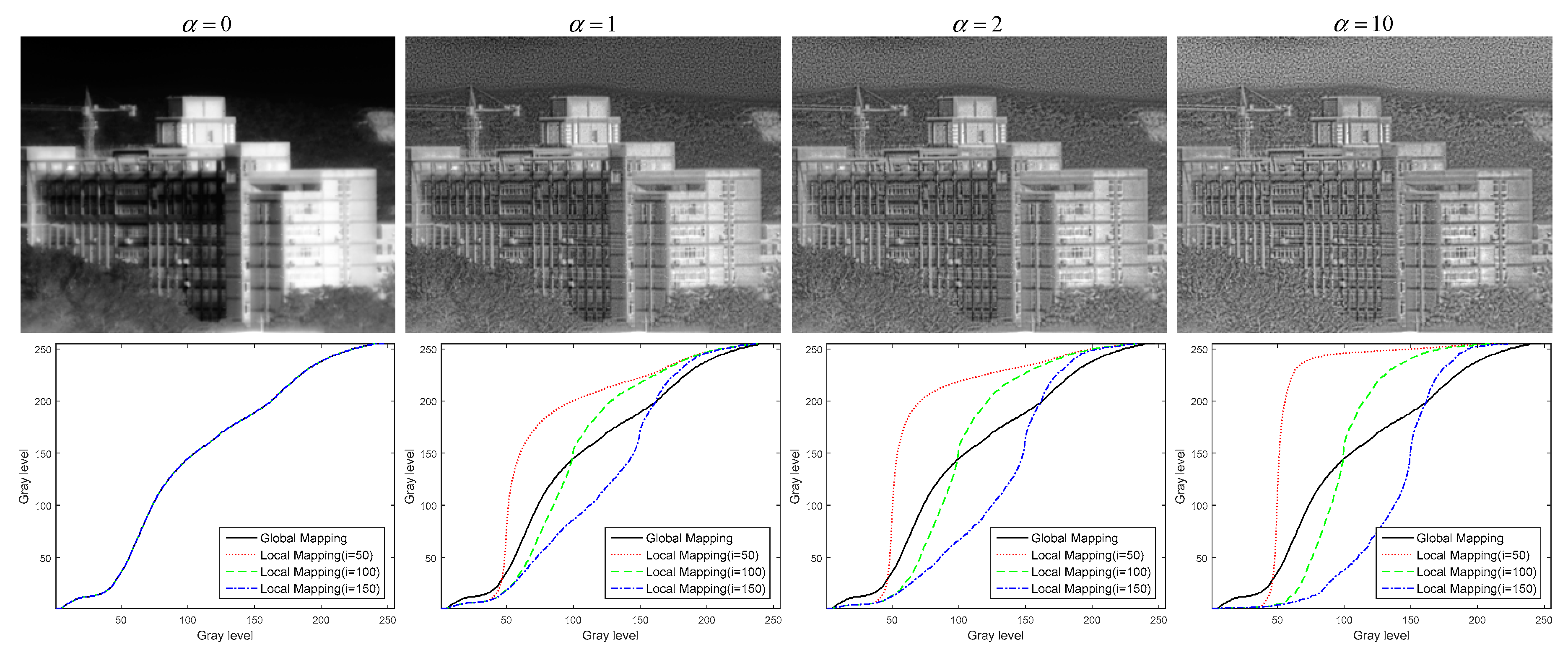
3.2. Local Enhancement

Local enhancement methods aim to enhance the contrast of each local area by using different mapping functions, which are computed based on the characteristics of the local areas. In this section, the local mapping function $T_i$ is defined to be the mapping function of the neighbors of pixels whose gray level is $i$. The histogram specification algorithm is utilized again to compute the local mapping function $T_i$. As for the local histogram, let $H_i=\left\{h_i(j)=h(i,j)/{\displaystyle {\sum }_{j=0}^{L-1}h(i,j)}|j=0,1,\cdots ,L-1\right\}$ be the normalized one row of the 2D histogram $H$ with index $i$, which indicates the gray level distribution of the neighbors of each pixel whose gray level is $i$ in the input image. Then, the corresponding cumulative distribution function is computed by the formula below.

$$C_i=\left\{c_i(j)={\displaystyle \sum _{k=0}^{k=j}{h}_i(k)}|j=0,1,\cdots ,L-1\right\}$$

(12)

As for the desired local histogram, similar to the desired 2D histogram, we assume that the desired local histogram satisfies the following Gaussian distribution probability density function [18].

$${\widehat{H}}_{i^{\prime }}=\left\{{\widehat{h}}_{i^{\prime }}(j^{\prime })|j^{\prime }=0,1,\cdots ,L-1\right\}$$

(13)

where ${\widehat{h}}_{i^{\prime }}(j^{\prime })=\frac{1}{\sqrt{2\pi }\sigma }{e}^{-\frac{{(j^{\prime }-i^{\prime })}^2}{2{\sigma }^2}}$

In addition, $\sigma$ is the weighted average value of the standard deviation of each row in the 2D histogram. The desired local histogram is also normalized by ${\widehat{h}}_{i^{\prime }}(j^{\prime })={\widehat{h}}_{i^{\prime }}(j^{\prime })/{\displaystyle {\sum }_{j^{\prime }=0}^{L-1}{\widehat{h}}_{i^{\prime }}(j^{\prime })}$. Then, we can compute the corresponding cumulative distribution function by using the formula below.

$${\widehat{C}}_{i^{\prime }}=\left\{{\widehat{c}}_{i^{\prime }}(j^{\prime })={\displaystyle \sum _{k=0}^{j^{\prime }}{\widehat{h}}_{i^{\prime }}(k)}|j^{\prime }=0,1,\cdots ,L-1\right\}$$

(14)

Once again, based on the histogram specification, the original local mapping function $T_i^{\prime }$ is computed according to the equation below.

$$T_i^{\prime }=\left\{t_i^{\prime }(j)=\underset{j^{\prime }\in \{0,1,\cdots ,L-1\}}{\arg \min }\left|c_i(j)-{\widehat{c}}_{i^{\prime }}(j^{\prime })\right||i=i^{\prime },j=0,1,\cdots ,L-1\right\}$$

(15)

An indisputable fact is that each local area is just a small part of the whole image. Therefore, not only the local areas but also the whole image have to be taken into consideration when enhancing the local contrast. This inspires us to update the original local mapping based on the global mapping function. When computing the optimal local mapping function, both local and global mapping functions have to be taken into account. To satisfy this condition, the preferred option is to find an optimal mapping function $T_i$, which is closer to $T_G$ and ensure the small residual $T_i-T_i^{\prime }$. The optimal local mapping function $T_i$ can be treated as the solution to a bi-criteria optimization problem. If the square of the Euclidean norm is used for the problem, the optimal local mapping function $T_i$ is computed by using the equation below.

$$T_i=\underset{T}{\arg \min }{\Vert T-T_G\Vert }_2^2+\alpha {\Vert T-T_i^{\prime }\Vert }_2^2$$

(16)

where $T$ is just an intermediate variable while $\alpha$ is a regularization parameter and varies over $\left[0,\infty \right)$. The solution to this quadratic optimization problem is shown below.

$$T_i=\left(\frac{1}{1+\alpha }\right)T_G+\left(\frac{\alpha }{1+\alpha }\right)T_i^{\prime }$$

(17)

Therefore, the optimal mapping function $T_i$ turns out to be a weighted average of $T_G$ and $T_i^{\prime }$. Simply by varying $\alpha$, $T_i$ takes on the optimal trade-off value between the two objectives. When $\alpha =0$, $T_i$ is equal to the global mapping function $T_G$. Therefore, the local enhancement result tends to be the same as the global enhancement result. However, as $\alpha$ goes to infinity, $T_i$ converges to the original local mapping function $T_i^{\prime }$. Thus, the local enhancement result usually results in over enhancement of the local contrast.

Since the local mapping function $T_i$ aims to enhance the contrast of the neighbors of the pixels whose gray level is $i$, each pixel in the input image is conversely one element of the neighbors of the pixels that belong to its neighborhood. Therefore, the local enhancement result of each pixel should be the average of the enhanced results using the mapping function of its neighbors. The local enhancement result $Y_L=\left\{y_L(m,n)|1\le m\le M,1\le n\le N\right\}$ of the input image is computed by the equation below.

$$y_L(m,n)=\frac{1}{W_r}{\displaystyle \sum _{k=-r}^r{\displaystyle \sum _{l=-r}^r{t}_{x(m+k,n+l)}(x(m,n))\times w_r(k,l)}}$$

(18)

where $W_r={\displaystyle \sum {\displaystyle \sum w_r(k,l)}}$ and $w_r(k,l)$ is defined as the element of the Gaussian weight matrix. The expression of $w_r(k,l)$ is shown below.

$$w_r(k,l)=\frac{1}{2\pi }{e}^{-(k^2+l^2)/2}$$

As shown in Figure 4, when $\alpha =0$, the local enhancement result is the same as the global enhancement result in Figure 3a. Thus, the local contrast is not enhanced. This is because the local mapping functions turn to coincide with the global mapping function. As the value of $\alpha$ gradually increases, the local mapping functions become different from the global mapping function, which results in a more enhanced local contrast. We empirically set $\alpha =1$ in the later experiments. Compared with the global enhancement result, local enhancement results look unnatural and the noise in homogeneous regions also emerges.

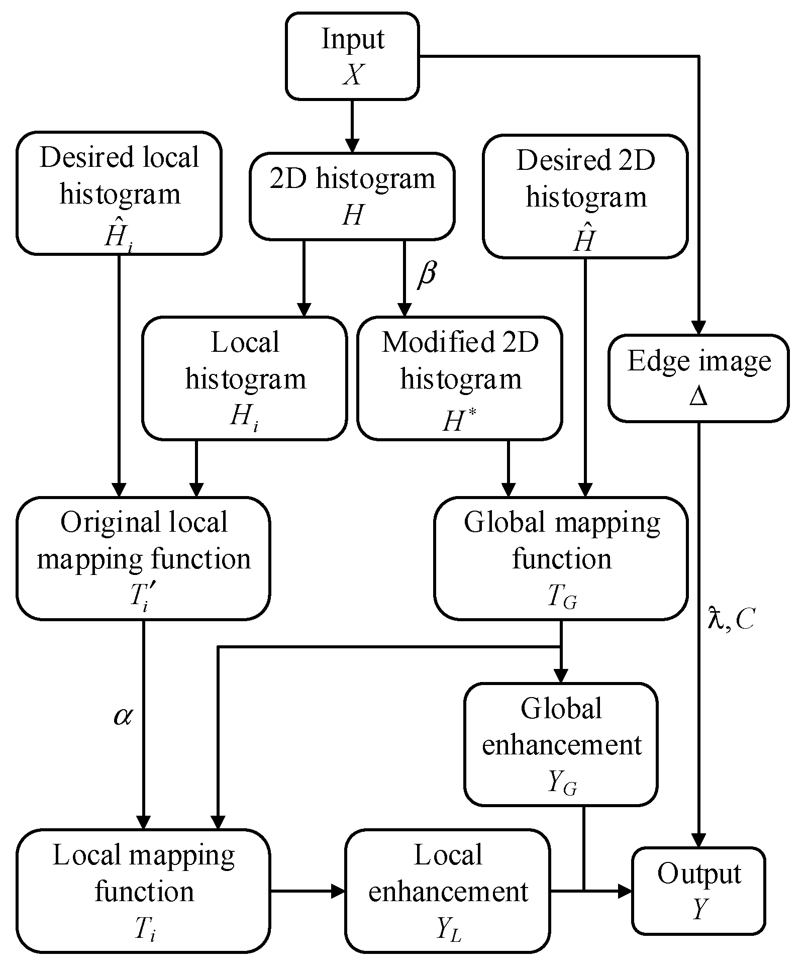
3.3. Optimized Enhancement

As described above, the global enhancement result improves the contrast of the input image without considering the characteristics of the input area. Thus, the contrast enhancement performance is limited. On the contrary, the local enhancement result shows much better performance on the local contrast improvement, but it looks unnatural and makes the noise emerge in homogeneous regions. Since the performance of global enhancement and local enhancement have complementary characteristics, the optimized enhancement is expected to combine the merits of both global and local enhancements. To achieve this goal, the optimized enhancement result $Y$ has to make a trade-off between two objectives: (1) the overall brightness variation should follow that of the global enhancement result and (2) the local contrast should follow that of the local enhancement result [5]. These two objectives are expressed as:

$$\begin{array}{l}1):Y^{\prime }=Y_G+E_G\hfill \\ 2):(Y^{\prime }-{\overline{Y}}^{\prime })./{\overline{Y}}^{\prime }=c(Y_L-{\overline{Y}}_L)./{\overline{Y}}_L+E_L\hfill \end{array}$$

(19)

where $Y^{\prime }$ is the desired image, ${\overline{Y}}^{\prime }$ is the set of average values of sub-blocks in $Y^{\prime }$, ${\overline{Y}}_L$ is the set of average values of sub-blocks in $Y_L$, $c$ is a constant and is defined as the contrast parameter, $E_G$ and $E_L$ are the lexicographically ordered sets of difference values in the condition of global brightness and local contrast similarity, and the operator $./$ indicates that the corresponding elements of the two sets are divided separately. The goal is to find a solution that can simultaneously minimize $E_G$ and $E_L$. Moreover, notice that the variation ranges of $E_G$ and $E_L$ are not of the same magnitude. The expression of the second objective is rewritten by the equation below.

$$Y^{\prime }-{\overline{Y}}^{\prime }=c(Y_L-{\overline{Y}}_L).\ast ({\overline{Y}}^{\prime }./{\overline{Y}}_L)+E_L^{\prime }$$

(20)

where $E_L^{\prime }=E_L.\ast {\overline{Y}}^{\prime }$

In this scenario, the operator $.\ast$ indicates that the corresponding elements of the two sets are multiplied separately. Therefore, the goal should be changed to find a solution that can simultaneously minimize $E_G$ and $E_L^{\prime }$. This is a bi-criteria optimization problem, and, in this paper, the square of the Frobenius norm is used to compute the solution below.

$$Y=\underset{Y^{\prime }}{\arg \min }{\Vert Y^{\prime }-Y_G\Vert }_F^2+\lambda {\Vert (Y^{\prime }-{\overline{Y}}^{\prime })-c(Y_L-{\overline{Y}}_L).\ast ({\overline{Y}}^{\prime }./{\overline{Y}}_L)\Vert }_F^2$$

(21)

where $\lambda$ is a regularization parameter and varies over $\left[0,\infty \right)$. The optimized enhancement result obtained by $\lambda =0$ is equal to the global enhancement result. Nevertheless, as $\lambda$ increases to infinity, it turns to resemble the local enhancement result. Therefore, a different optimized enhancement result is obtained according to $\lambda$ and $c$. Considering the region characteristics of the input image, larger $\lambda$ and $c$ are needed for the detailed regions to get local contrast enhanced, but smaller $\lambda$ and $c$ are more suitable for the homogeneous regions. Thus, $\lambda$ and $c$ should be a region with adaptive variables and should be represented as the component of $\mathrm{ƛ}=\left\{\lambda (m,n)|1\le m\le M,1\le n\le N\right\}$ and $C=\left\{c(m,n)|1\le m\le M,1\le n\le N\right\}$ instead of a constant. Moreover, notice that the value of ${\overline{Y}}^{\prime }$ is unknown and the desired image $Y^{\prime }$ satisfies the objective functions in Equation (19). We assume that the average value of the desired image is approximately equal to that of the global enhancement image $({\overline{Y}}^{\prime }\approx {\overline{Y}}_G)$. Then Equation (21) is rewritten as the formula below.

$$Y=\underset{Y^{\prime }}{\arg \min }{\Vert Y^{\prime }-Y_G\Vert }_F^2+{\Vert \mathrm{ƛ}.\ast \left[(Y^{\prime }-{\overline{Y}}_G)-C.\ast (Y_L-{\overline{Y}}_L).\ast ({\overline{Y}}_G./{\overline{Y}}_L)\right]\Vert }_F^2$$

(22)

The optimal solution of Equation (22) is shown below.

$$Y=Y_G./(\mathbf{1}+\mathrm{ƛ})+\left[{\overline{Y}}_G+C.\ast (Y_L-{\overline{Y}}_L).\ast ({\overline{Y}}_G./{\overline{Y}}_L)\right].\ast \mathrm{ƛ}./(\mathbf{1}+\mathrm{ƛ})$$

(23)

where $\mathbf{1}$ is the $M\times N$ one matrix. As shown in Equation (23), the first term indicates that the optimized enhancement result resembles the global enhancement result, and the second term adds the weighted local contrast of the local enhancement result to the average value of the global enhancement result. Therefore, based on the proposed method, the brightness variation of the global enhancement result and the local contrast of the local enhancement result are merged into the optimized enhancement result. It is clear that the characteristics of the optimized enhancement result are related to the values of $\mathrm{ƛ}$ and $C$. In this paper, $C$ and $\mathrm{ƛ}$ are adaptively determined based on the edge information of the input image. The edge information $\Delta$ is first computed by using the Sobel operator and then is linearly mapped to the same dynamic range of the output image. The value of each element in $\mathrm{ƛ}$ and $C$ are defined to be positively correlated with the corresponding value of edge information and are computed by the equation below.

$$\begin{array}{l}\mathrm{ƛ}={\lambda }_0\times \Delta \hfill \\ C=c_0\Delta ./(2c_0-2+\Delta )\hfill \end{array}$$

(24)

where ${\lambda }_0$ and $c_0$ are user-defined parameters and are empirically set as ${\lambda }_0=0.1$ and $c_0=2$ in the later experiments.

Figure 5 shows the map of edge information $\Delta$, the optimized enhancement result $Y$, and the map of edge information of $Y$. All these edge information maps are computed by applying the Sobel operator to the corresponding images and the values are non-negative. It can be clearly seen from the two edge information maps so that the edge information in Figure 5c looks much clearer than that in Figure 5a. Besides this, the pixels containing edge information have the same coordinates in these two edge information maps. This indicates that the enhancement result of our proposed method can preserve and enhance the edge information of the original image. In addition to that, for the detailed regions, the edge information in Figure 5c is more abundant than that in Figure 5a. In addition, for the homogeneous regions, the edge information in Figure 5c is similar to that in Figure 5a. This indicates that the proposed method is able to adaptively enhance the contrast in detailed regions and keep the contrast in homogeneous regions unchanged. For a better understanding of our proposed method (Algorithm 1), a brief pseudo code of the proposed method is given as follows.

Algorithm 1: Optimized Contrast Enhancement Method.

Input: original infrared image $X$ Output: enhanced image $Y$ 1. Pre-process $X$ to be the 8-bit image 2. Calculate the 2D histogram $H$ of image $X$ based on Equation (2), the parameter $r$ determines the size of the neighbor region 3. Obtain the clipped 2D histogram $H^{\ast }$ by clipping $H$ and redistributing the exceeded pixels, normalize $H^{\ast }$, the clip point is determined by the parameter $\beta$ 4. Calculate the global mapping function $T_G$ based on the cumulative distribution functions of $H^{\ast }$ and the desired uniformly distributed 2D histogram $\widehat{H}$ using Equation (10) 5. Map the image $X$ to the global enhancement result $Y_G$ using Equation (11) 6. Construct the desired local histogram ${\widehat{H}}_i$ based on the Gaussian distribution probability density function using Equation (13) 7. Calculate the original local mapping function ${T^{\prime }}_i$ based on the cumulative distribution functions of $H_i$ and the desired local 2D histogram ${\widehat{H}}_{i^{\prime }}$ using Equation (15) 8. Solve the bi-criteria optimization function in Equation (16), obtain the optimal local mapping function $T_i$, $\alpha$ is introduced to be a regularization parameter 9. Map the image $X$ to the local enhancement result $Y_L$ using Equation (18) 10. Calculate $\mathrm{ƛ}$ and $C$ based on Equation (24), ${\lambda }_0$ and $c_0$ are the introduced parameters, $\Delta$ is computed by applying the Sobel operator to $X$ 11. Solve the bi-criteria optimization function in Equation (22), obtain the optimized contrast enhancement result $Y$, $\mathrm{ƛ}$, and $C$ are the regularization parameter set and the contrast parameter set 12. Return $Y$

4. Experimental Results and Discussion

In this section, experiments are conducted to evaluate the performance of the proposed method and the results were compared with those of three LCE methods: BCCE, ABMHE, and LGGSF. All these methods are applied to enhance the contrast of six different infrared images, which are captured by a cooled mid-wave infrared camera. The resolution of these images are $320\times 256$ and the pre-processed 8-bit images are shown in Figure 6 as a reference. All these experiments are performed on a PC with Intel(R) Core(TM) i7 CPU(3.40 GHz) and 16.00 GB RAM using MATLAB on a Windows 10 operation system.

4.1. Parameter Setting

There are five parameters introduced in our proposed method. For these parameters, the values we chose are given in the above section. In this paper, we conduct a further discussion on the value set. The parameter $r$ determines the size of the neighbor region when calculating the 2D histogram. A larger value of $r$ means more neighbor pixels are taken into account and also corresponds to the higher computational complexity. Thus, we set $r=2$ in our proposed method. $\beta$ is introduced to reduce the over-enhancement of the global enhancement result in Section 3.1. The value of $\beta$ is recommended to be set within the range of $\left[0.1,1\right]$. In our experiments, for the images with a resolution of $320\times 256$, we set $\beta =0.2$. For other images with higher resolution, a larger $\beta$ value is recommended. As for the parameter $\alpha$, the effect of different $\alpha$ values on the local enhancement results in Section 3.2 can be seen in Figure 4. A larger value of $\alpha$ means more local contrast is enhanced. In the meantime, the noise in the homogeneous regions is also enhanced. Thus, we set $\alpha =1$ in our proposed method to make a trade-off between the local contrast enhancement and the noise amplification. The parameters ${\lambda }_0$ and $c_0$ are introduced to determine the regularization parameter set $\mathrm{ƛ}$ and the contrast parameter set $C$ based on the edge information $\Delta$. As discussed before, when the value of $\mathrm{ƛ}$ approaches zero, the optimized enhancement result tends to keep the brightness variation of the global enhancement result. On the contrary, if the value of $\mathrm{ƛ}$ increases to infinity, the optimized enhancement result turns to keep the local contrast of the local enhancement result. Considering the noise suppression, we set ${\lambda }_0=0.1$ in our experiments. If more local contrast enhancement is required, ${\lambda }_0$ can be set to a larger value. From the definition of $C$ in Equation (24), it is clear that the values of the components in $C$ are within the range of $\left[0,c_0\right]$. Thus, the value of $c_0$ represents the maximum contrast enhancement ratio. In our experiments, we empirically set $c_0=2$ to obtain the proper contrast enhancement.

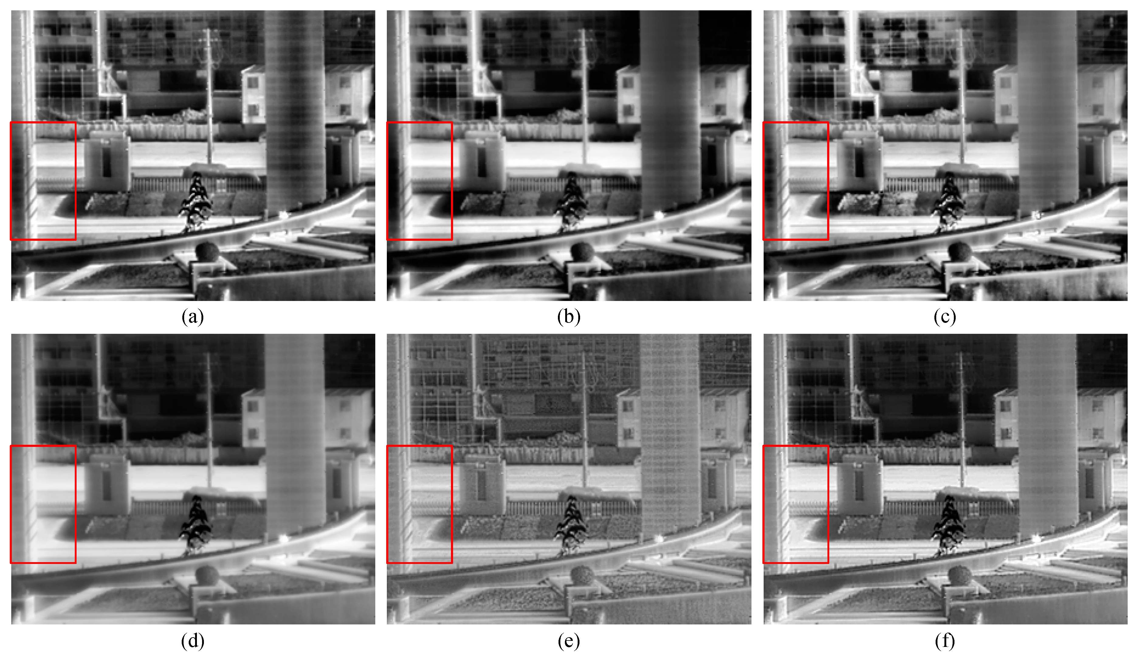
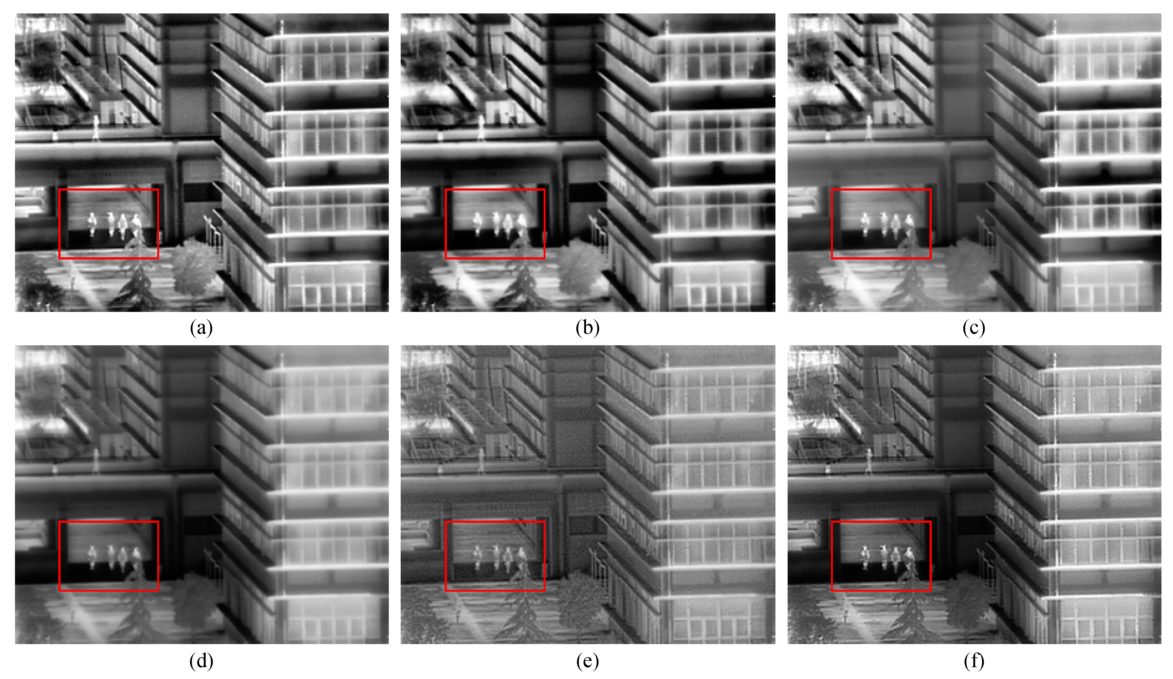
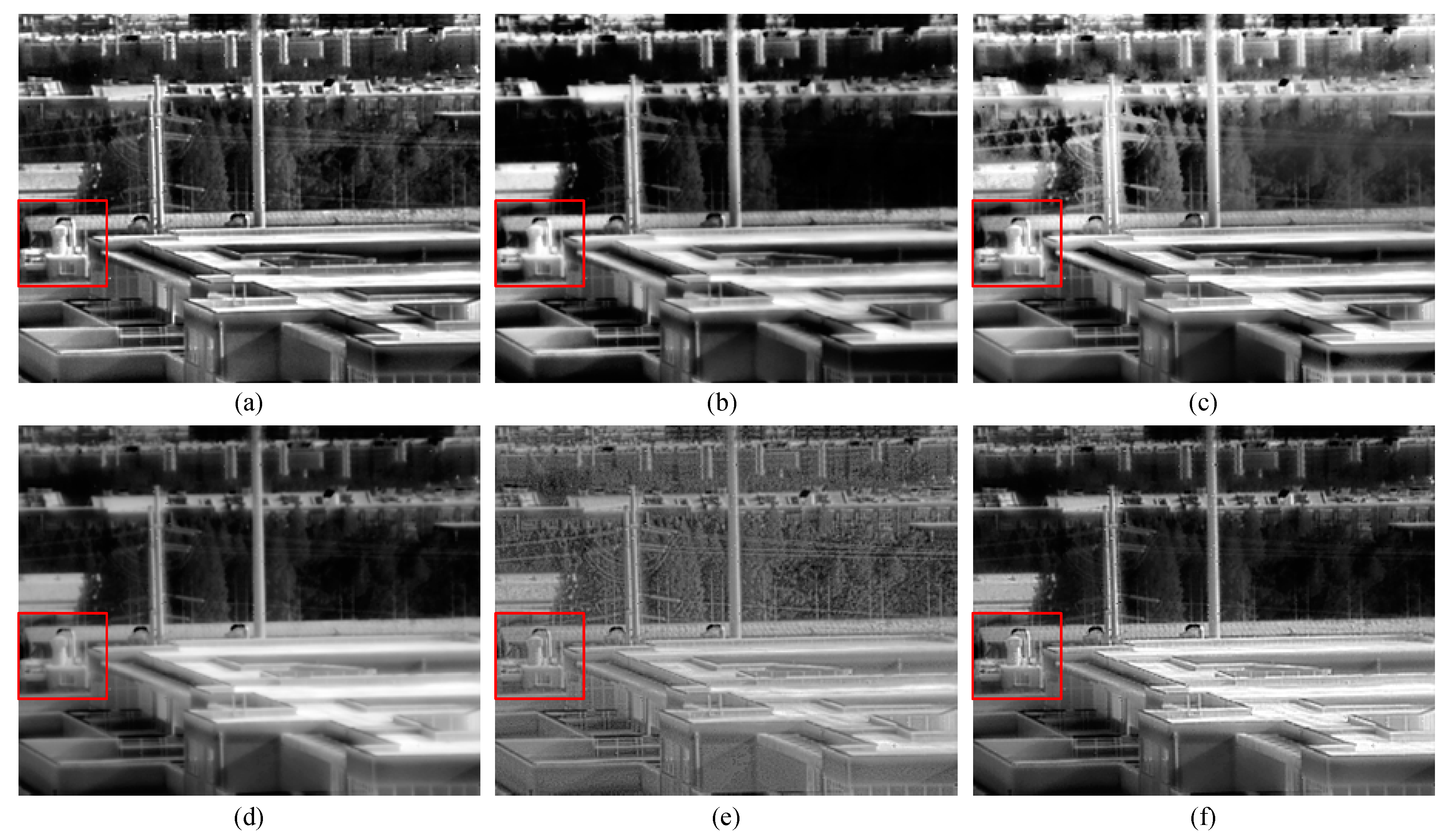
4.2. Qualitative Evaluation

The enhancement results of the reference images in Figure 6 using BCCE, ABMHE, LGGSF, and the proposed method are shown in Figure 7, Figure 8, Figure 9, Figure 10, Figure 11 and Figure 12. The numbers of horizontal and vertical divisions of the image for BCCE and LGGSF are set to be $k_1=k_2=7$. The clip limit parameter and local contrast enhancement factor for BCCE are set as $\beta =0.01$ and $\alpha =1.2$. The local contrast enhancement factor for LGGSF is set as $\alpha =8$. For the ABMHE method, the block size is set to be $64\times 64$. The horizontal and vertical steps are set to be one-quarter of the block size.

As shown in these figures, the intermediate global and local enhancement results are given together with the optimized result. For each test image, the final enhancement result of our proposed method is the optimized result of the intermediate enhancement results. It can be seen that the global enhancement results improve the visual quality with no artifacts, but the local contrast is not well enhanced. In the local enhancement results, the enhanced local contrast is enhanced but looks unnatural and the noise in homogeneous regions also emerges. The optimized results adaptively combine the merits of both global and local enhancement results. Therefore, the results improve the visual quality with an enhanced local contrast and no artifacts.

As shown in Figure 7, we can clearly find that the edge information of the buildings in the result of the proposed method and BCCE looks clearer than the others. The result of ABMHE causes over-enhancement in the trees of the image. However, in the result of LGGSF, more details of the trees and mountain are lost. In the region marked by the red rectangle, BCCE amplifies the noise and ABMHE causes blocking artifacts.

In Figure 8, as shown in the region marked by the red rectangle, the result of LGGSF shows over-enhancement artifacts and that of ABMHE lost some details in the darker area. It can be observed that there is brightness distortion in the enhancement results of BCCE, ABMHE, and LGGSF. Once again, BCCE and the proposed method produces clearer visual quality than ABMHE and LGGSF.

In Figure 9, over-enhancement artifacts appear in the homogeneous regions of the results of BCCE and ABMHE. The noise is also amplified in the result of BCCE. We can also observe that the tower crane marked by the red rectangle looks fuzzy in the results of BCCE, ABMHE, and LGGSF. The result of the proposed method looks more natural and clearer than that of the others.

In Figure 10, the result of BCCE appears to have severe brightness distortion in the region marked by the red rectangle and other homogeneous regions. This distortion also appears in the results of ABMHE and LGGSF. In addition, LGGSF also causes artifacts in some homogeneous regions. The enhancement result of the proposed method preserves the naturalness of the original image and gives better local contrast enhancement with brightness distortion.

In Figure 11, it is clear that the people in the region marked by the red rectangle of the proposed method are clearer than that of the BCCE, ABMHE, and LGGSF. Additionally, the result of the proposed method produces more legible edge information than the other methods.

In Figure 12, there are no large homogeneous regions in the scene. Thus, the brightness distortion is not apparent in the results of BCCE, ABMHE, and LGGSF. However, the enhancement results of ABMHE and LGGSF still look unnatural at the regions of the trees. We can see more details lost in that area. BCCE performs best in terms of local contrast enhancement. The proposed method is slightly inferior to BCCE. As observed in the region marked by the red rectangle, the objects in the results of ABMHE and LGGSF look fuzzy. BCCE and the proposed method give better visual quality.

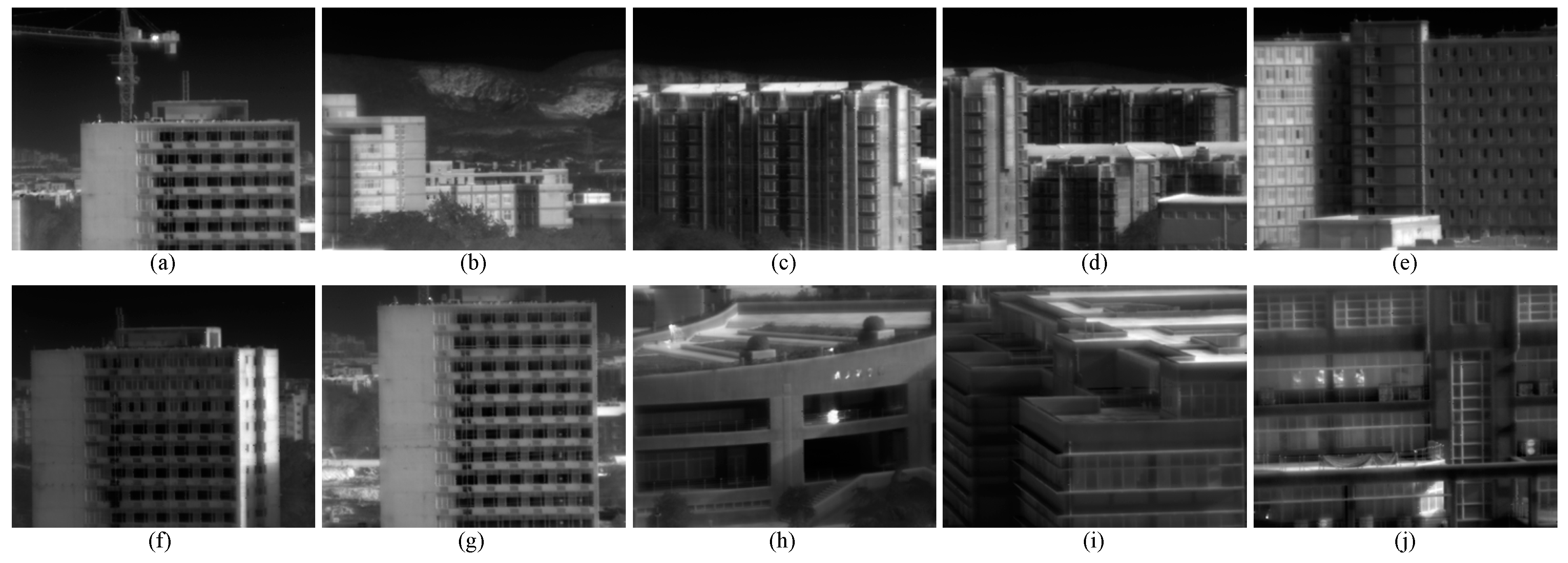
4.3. Quantitative Evaluation

For further evaluation, some objective assessment metrics are employed to numerically evaluate the performance of the proposed method. The metrics used in this paper are the measure of enhancement by entropy (EMEE) [39], structural similarity (SS) [40], no-reference structural sharpness (NRSS) [41], and the lightness order error (LOE) [38].

EMEE is defined based on the concept of entropy, which calculates the average ratio of maximum to minimum intensities in each block in decibels. The definition of EMEE is shown below.

$$EMEE(I)=\frac{1}{k_1{k}_2}{\displaystyle \sum _{k=1}^{k_1}{\displaystyle \sum _{l=1}^{k_2}\alpha {(\frac{I_{k,l}^{\max }}{I_{k,l}^{\min }+c})}^{\alpha }\ln (\frac{I_{k,l}^{\max }}{I_{k,l}^{\min }+c})}}$$

(25)

where $k_1$ and $k_2$ are the numbers of blocks the given image $I$ is divided in the horizontal and vertical direction, $I_{k,l}^{\max }$ and $I_{k,l}^{\min }$ are, respectively, the maximum and minimum intensity of the block $(k,l)$, $\alpha$ is an additional parameter, and $c$ is a small constant to avoid dividing by zero. Generally, the larger EMEE indicates better contrast of the given image. In this paper, we set $\alpha =0.2$, $c=0.0001$, and $8\times 8$ for the block size.

SS is based on the assumption that natural images are highly structured and is defined as the equation below.

$$SS(I_o,I_e)=\frac{{\sigma }_{I_o,I_e}+c}{{\sigma }_{I_o}{\sigma }_{I_e}+c}$$

(26)

where $I_o$ and $I_e$ are, respectively, the original image and enhanced image, ${\sigma }_{I_o,I_e}$ is the covariance of $I_o$, and $I_e$, ${\sigma }_{I_o}$, and ${\sigma }_{I_e}$ are the corresponding standard deviation, $c$ is a small constant to avoid dividing by zero, and ${\sigma }_{I_o,I_e}$ is estimated by the equation below.

$${\sigma }_{I_o,I_e}=\frac{1}{N-1}{\displaystyle \sum _{i=1}^N(I_o(i)-{\mu }_{I_o})(I_e(i)-{\mu }_{I_e})}$$

(27)

where $N$ is the number of pixels in the images and ${\mu }_{I_o}$ and ${\mu }_{I_e}$ are, respectively, the mean intensity of $I_o$ and $I_e$. It is clear that SS indicates the structural similarity of the enhanced image when compared to the original image. The larger SS means the enhanced image is more close to the original image in terms of structure.

NRSS is defined based on the well-known SSIM (structural similarity index measurement) [42] to indicate the structural sharpness of the given image, which is defined by the equation below.

$$NRSS(I)=1-\frac{1}{K}{\displaystyle \sum _{i=1}^{K}SSIM(B_i^{G_I},B_i^{G_{F(I)}})}$$

(28)

where $B_i^{G_I}$ is one of the $K$ overlapped sub-blocks with higher variations in $G_I$, $G_I$ is the gradient image of the given image $I$ and is calculated by applying Sobel operator to the given image, and $F(•)$ is the 2D Gaussian-blurred function. Large NRSS means that the given image looks clear and is rich in details. In our experiments, the block size is set to be $32\times 32$ and the step is set to half the block size, and $K$ is set to be half of the total number of the overlapped sub-blocks.

LOE is defined based on the lightness order error between the original image and the enhanced image. The definition of LOE is shown below.

$$\{\begin{array}{l}LOE=\frac{1}{MN}{\displaystyle \sum _{i=1}^M{\displaystyle \sum _{j=1}^{N}RD(i,j)}}\hfill \\ RD(i,j)={\displaystyle \sum _{m=1}^M{\displaystyle \sum _{n=1}^N(U(I_o^D(i,j),I_o^D(m,n))\oplus U(I_e^D(i,j),I_e^D(m,n)))}}\hfill \\ U(x,y)=\{\begin{array}{l}\begin{array}{cc}1& forx\ge y\end{array}\hfill \\ \begin{array}{cc}0& else\end{array}\hfill \end{array}\hfill \end{array}$$

(29)

where $U(x,y)$ is the unit step function, $\oplus$ is the exclusive or operator, and $I_o^D$ and $I_e^D$ are, respectively, the down-sampled version of $I_o$ and $I_e$ to reduce the computational complexity. The ratio between the size of the original image and that of the down-sampled image is set as $r=16$ in our experiments. For the better naturalness preservation of the original image, the LOE value of the enhanced result is expected to be smaller.

As shown in

Table 1. The values of EMEE, SS, NRSS, and LOE of the enhanced result obtained by BCCE, ABMHE, LGGSF, and the proposed method.

Metrics	Methods	Test Images in Figure 6						Average
		(a)	(b)	(c)	(d)	(e)	(f)
EMEE	Original	0.2190	0.2560	0.1442	0.1569	0.1534	0.2482	0.1963
	BCCE	0.5789	1.0363	0.5245	0.5367	0.5252	1.1947	0.7327
	ABMHE	1.3581	2.9490	1.8895	1.0964	0.9739	2.3617	1.7714
	LGGSF	0.1955	1.7445	0.1497	1.0375	0.3348	1.2646	0.7878
	Proposed	0.3172	0.9685	0.4910	1.0302	1.0707	1.6823	0.9267
SS	Original	1	1	1	1	1	1	1
	BCCE	0.8409	0.8690	0.8728	0.8193	0.7214	0.7821	0.8176
	ABMHE	0.8449	0.9446	0.8966	0.8455	0.7213	0.7894	0.8404
	LGGSF	0.9151	0.8481	0.9857	0.7756	0.8425	0.6577	0.8375
	Proposed	0.9339	0.9689	0.9866	0.9761	0.9761	0.9028	0.9574
NRSS	Original	0.8248	0.7536	0.8511	0.7534	0.8160	0.7779	0.7961
	BCCE	0.9292	0.9069	0.9392	0.8782	0.8645	0.9252	0.9072
	ABMHE	0.8375	0.7477	0.8397	0.7716	0.7641	0.7780	0.7898
	LGGSF	0.8829	0.8365	0.8770	0.8426	0.7933	0.8474	0.8466
	Proposed	0.9520	0.8631	0.9365	0.9141	0.9307	0.9033	0.9166
LOE	Original	0	0	0	0	0	0	0
	BCCE	59.15	39.71	50.40	75.85	85.51	55.51	61.02
	ABMHE	36.54	24.64	52.44	69.38	82.93	40.95	51.15
	LGGSF	30.86	45.24	9.97	76.26	58.41	83.01	50.63
	Proposed	9.81	10.69	8.68	11.29	13.61	9.41	10.58

, the highest values of EMEE, SS, NRSS, and the lowest values of LOE are marked in bold. As for the EMEE values, ABMHE gives almost the highest values for the test images among the four methods. However, ABMHE also produces over-enhancement artifacts in some regions, as shown in Figure 7, Figure 8, Figure 9, Figure 10, Figure 11 and Figure 12. The BCCE treats all six images without discrimination. Thus, the noise in the homogeneous regions are amplified, as shown in Figure 7a and Figure 9a. LGGSF and the proposed method give relatively lower EMEE values for Figure 6a,c and higher values for the other images. However, LGGSF may cause over-enhancement or contrast reduction in some regions, such as the regions in Figure 7c and Figure 8c. This situation also appears in the enhanced result of ABMHE, which is caused by the sub-block classification. The proposed method performs better in this regard without over-enhancement or contrast reduction. Comparison of SS values shows that the proposed method outperforms the other methods with the highest values. This indicates that the structure of the enhancement results of the proposed method is most similar to the original images. Comparison of NRSS values shows that BCCE and the proposed method gives higher values than ABMHE and LGGSF. This is also demonstrated by the clearer enhancement results in Figure 7, Figure 8, Figure 9, Figure 10, Figure 11 and Figure 12. The clearer appearance mainly benefits from the local enhancement mechanism of BCCE and the proposed method. Comparison of LOE values shows that the proposed method performs best on naturalness preservation than the other three methods. The higher LOE values of BCCE, ABMHE, and LGGSF are caused by the block-based principle and the neglect of global characteristics. All values of these metrics demonstrate that the proposed method outperforms the other methods in terms of structural similarity, local contrast enhancement, and naturalness preservation.

These four methods are also applied to another 10 infrared images shown in Figure 13 for the quantitative evaluation. The values of the objective assessment metrics are given in

Table 2. The values of EMEE, SS, NRSS, and LOE of the enhanced results obtained by applying the four methods to the 10 infrared images.

Metrics	Methods	Test Images in Figure 13										Average
		(a)	(b)	(c)	(d)	(e)	(f)	(g)	(h)	(i)	(j)
EMEE	Original	0.2017	0.1718	0.1910	0.2201	0.2009	0.2112	0.2313	0.1584	0.1704	0.2252	0.1982
	BCCE	0.7699	0.5290	0.4959	0.5346	0.6480	0.7209	0.9094	0.4127	0.5627	1.1605	0.6744
	ABMHE	1.4387	1.4713	2.3195	2.2688	2.1855	1.4585	0.8927	1.6636	1.0797	1.5135	1.6292
	LGGSF	0.3383	0.1915	0.6501	0.8170	1.7540	0.6360	0.7267	0.5487	0.7851	0.9432	0.7391
	Proposed	2.1975	0.1959	0.3858	0.2545	1.6005	3.0638	6.4672	0.3221	0.5787	2.0923	1.7158
SS	Original	1	1	1	1	1	1	1	1	1	1	1
	BCCE	0.8629	0.8657	0.8617	0.9225	0.7657	0.7201	0.8058	0.7947	0.7437	0.7913	0.8134
	ABMHE	0.9231	0.8696	0.7928	0.9282	0.7832	0.6536	0.8687	0.8628	0.7741	0.8376	0.8294
	LGGSF	0.9417	0.9559	0.8061	0.8775	0.6383	0.7552	0.8582	0.7863	0.6239	0.8463	0.8089
	Proposed	0.9845	0.9660	0.9356	0.9628	0.9462	0.8621	0.9672	0.9755	0.9352	0.9324	0.9468
NRSS	Original	0.8232	0.8274	0.8111	0.7829	0.8500	0.7712	0.8255	0.7396	0.7721	0.8229	0.8026
	BCCE	0.9424	0.9367	0.9647	0.9323	0.9508	0.9451	0.9464	0.8733	0.8794	0.9214	0.9293
	ABMHE	0.8199	0.8322	0.8382	0.8016	0.8622	0.8444	0.8277	0.7380	0.7604	0.8168	0.8141
	LGGSF	0.8519	0.8914	0.8857	0.8614	0.8783	0.8748	0.8567	0.8112	0.7855	0.8257	0.8523
	Proposed	0.9212	0.9629	0.9410	0.9211	0.9641	0.9417	0.9343	0.8648	0.9285	0.9085	0.9288
LOE	Original	0	0	0	0	0	0	0	0	0	0	0
	BCCE	45.40	57.08	46.63	40.82	63.08	45.72	60.36	66.37	86.63	57.86	57.00
	ABMHE	49.70	41.16	45.99	35.26	54.89	44.58	47.94	48.20	76.66	46.59	49.10
	LGGSF	24.49	29.65	36.88	39.47	59.29	35.55	47.83	61.39	92.27	41.38	46.82
	Proposed	7.24	11.31	6.95	7.34	14.18	8.56	15.53	8.38	10.67	10.40	10.06

.

In Table 2, it can be seen that the proposed method gives lower EMEE values for the images that contain more homogeneous regions or fewer detail regions, which is the same as those EMEE values in Table 1. The NRSS values of the proposed method are close to those of BCCE and higher than those of ABMHE and LGGSF. Comparison of SS and LOE values shows that the proposed method always gives the highest SS values and lowest LOE values. This means the proposed method has better performance than the other methods for preserving the naturalness and structure of the original images. All these quantitative evaluation values demonstrate that the proposed method has better performance on adaptive contrast enhancement, structural similarity, visual quality improvement, and naturalness preservation.

The average computation time for the four methods to process the test images in Figure 6 and Figure 13 are given in

Table 3. The average computation time in seconds of the four methods on the test images.

Method	BCCE	ABMHE	LGGSF	Proposed
Time	0.0865	2.4670	0.1347	0.8959

. As shown in the table, the average computation time of BCCE is lower than the other methods. For LGGSF, the sub-block classification and labeling lead to more time consumption than BCCE. In our proposed method, the utilization of the histogram specification and the local contrast enhancement part require more computation time than LGGSF and BCCE. In ABMHE, the overlapped sub-blocks and the sub-block search operations make it the most time-consuming method among the four methods.

5. Conclusions

In this paper, we proposed an optimized contrast enhancement method for the visual quality improvement of infrared images. The proposed method produces enhanced images by making an optimal compromise between the global and local enhancement results that consider the edge information of the original image. In the proposed method, based on the 2D histogram of the original image, the global and local enhancement results are obtained by applying histogram specification globally and locally. Then, an objective function is constructed with global brightness and local contrast constrained conditions. The desired image is obtained by finding an analytical solution for the quadratic optimization problem. The regularization parameter set $\mathrm{ƛ}$ and contrast parameter set $C$ for the optimization function are adaptively determined by the edge information of the original image. Experiments are conducted for the qualitative and quantitative assessment of the proposed method with three block-based methods for comparison. Experimental results demonstrate that the proposed method produces better visual quality improvement in terms of structural similarity, naturalness preservation, and local contrast enhancement.

References

1. Cao, Y.; Yang, M.Y.; Tisse, C.L. Effective Strip Noise Removal for Low-Textured Infrared Images Based on 1-D Guided Filtering. IEEE Trans. Circuits Syst. Video Technol. 2016, 26, 2176–2188. [Google Scholar] [CrossRef]
2. Ring, E.; Ammer, K. Infrared thermal imaging in medicine. Physiol. Meas. 2012, 33, R33. [Google Scholar] [CrossRef]
3. Liu, C.; Sui, X.; Liu, Y.; Kuang, X.; Gu, G. FPN estimation based nonuniformity correction for infrared imaging system. Infrared Phys. Technol. 2019, 96, 22–29. [Google Scholar] [CrossRef]
4. Kim, J.-H.; Kim, J.-H.; Jung, S.-W.; Ko, S.-J.; Noh, C.-K. Novel contrast enhancement scheme for infrared image using detail-preserving stretching. OPTICE 2011, 50, 077002. [Google Scholar]
5. Song, K.S.; Kang, M.G. Optimized Tone Mapping Function for Contrast Enhancement considering Human Visual Perception System. IEEE Trans. Circuits Syst. Video Technol. 2018. [Google Scholar] [CrossRef]
6. Gonzalez, R.C.; Woods, R.E.; Eddins, S.L. Digital Image Processing Using MATLAB; Pearson-Prentice-Hall: Upper Saddle River, NJ, USA, 2004; Volume 624. [Google Scholar]
7. Lin, C.-L. An approach to adaptive infrared image enhancement for long-range surveillance. Infrared Phys. Technol. 2011, 54, 84–91. [Google Scholar] [CrossRef]
8. Vickers, V.E. Plateau equalization algorithm for real-time display of high-quality infrared imagery. OPTICE 1996, 35, 1921–1927. [Google Scholar] [CrossRef]
9. Wang, B.-J.; Liu, S.-Q.; Li, Q.; Zhou, H.-X. A real-time contrast enhancement algorithm for infrared images based on plateau histogram. Infrared Phys. Technol. 2006, 48, 77–82. [Google Scholar] [CrossRef]
10. Liang, K.; Ma, Y.; Xie, Y.; Zhou, B.; Wang, R. A new adaptive contrast enhancement algorithm for infrared images based on double plateaus histogram equalization. Infrared Phys. Technol. 2012, 55, 309–315. [Google Scholar]
11. Li, S.; Jin, W.; Li, L.; Li, Y. An improved contrast enhancement algorithm for infrared images based on adaptive double plateaus histogram equalization. Infrared Phys. Technol. 2018, 90, 164–174. [Google Scholar] [CrossRef]
12. Kim, Y.-T. Contrast enhancement using brightness preserving bi-histogram equalization. IEEE Trans. Consum. Electron. 1997, 43, 1–8. [Google Scholar]
13. Wang, Y.; Chen, Q.; Zhang, B. Image enhancement based on equal area dualistic sub-image histogram equalization method. IEEE Trans. Consum. Electron. 1999, 45, 68–75. [Google Scholar] [CrossRef]
14. Chen, S.-D.; Ramli, A.R. Contrast enhancement using recursive mean-separate histogram equalization for scalable brightness preservation. IEEE Trans. Consum. Electron. 2003, 49, 1301–1309. [Google Scholar] [CrossRef]
15. Huang, J.; Ma, Y.; Zhang, Y.; Fan, F. Infrared image enhancement algorithm based on adaptive histogram segmentation. Appl. Opt. 2017, 56, 9686–9697. [Google Scholar] [CrossRef]
16. Wan, M.; Gu, G.; Qian, W.; Ren, K.; Chen, Q.; Maldague, X. Infrared Image Enhancement Using Adaptive Histogram Partition and Brightness Correction. Remote Sens. 2018, 10, 682. [Google Scholar] [CrossRef]
17. Arici, T.; Dikbas, S.; Altunbasak, Y. A histogram modification framework and its application for image contrast enhancement. IEEE Trans. Image Process. 2009, 18, 1921–1935. [Google Scholar] [CrossRef]
18. Xiao, B.; Tang, H.; Jiang, Y.; Li, W.; Wang, G. Brightness and contrast controllable image enhancement based on histogram specification. Neurocomputing 2018, 275, 2798–2809. [Google Scholar] [CrossRef]
19. Zuiderveld, K. Contrast Limited Adaptive Histogram Equalization. In Graphics Gems; Elsevier: Amsterdam, The Netherlands, 1994; pp. 474–485. ISBN 0-12-336155-9. [Google Scholar]
20. Kim, J.-Y.; Kim, L.-S.; Hwang, S.-H. An advanced contrast enhancement using partially overlapped sub-block histogram equalization. IEEE Trans. Circuits Syst. Video Technol. 2001, 11, 475–484. [Google Scholar]
21. Branchitta, F.; Diani, M.; Corsini, G.; Porta, A. Dynamic-range compression and contrast enhancement in infrared imaging systems. OPTICE 2008, 47, 076401. [Google Scholar] [CrossRef]
22. Yuan, L.T.; Swee, S.K.; Ping, T.C. Infrared image enhancement using adaptive trilateral contrast enhancement. Pattern Recognit. Lett. 2015, 54, 103–108. [Google Scholar] [CrossRef]
23. Wang, Y.; Pan, Z. Image contrast enhancement using adjacent-blocks-based modification for local histogram equalization. Infrared Phys. Technol. 2017, 86, 59–65. [Google Scholar] [CrossRef]
24. Li, S.; Jin, W.; Wang, X.; Li, L.; Liu, M. Contrast Enhancement Algorithm for Outdoor Infrared Images based on Local Gradient-grayscale Statistical Feature. IEEE Access 2018, 6, 57341–57352. [Google Scholar] [CrossRef]
25. Branchitta, F.; Diani, M.; Corsini, G.; Romagnoli, M. New technique for the visualization of high dynamic range infrared images. OPTICE 2009, 48, 096401. [Google Scholar] [CrossRef]
26. Zuo, C.; Chen, Q.; Liu, N.; Ren, J.; Sui, X. Display and detail enhancement for high-dynamic-range infrared images. OPTICE 2011, 50, 127401. [Google Scholar] [CrossRef]
27. Liu, N.; Zhao, D. Detail enhancement for high-dynamic-range infrared images based on guided image filter. Infrared Phys. Technol. 2014, 67, 138–147. [Google Scholar] [CrossRef]
28. Liu, N.; Chen, X. Infrared image detail enhancement approach based on improved joint bilateral filter. Infrared Phys. Technol. 2016, 77, 405–413. [Google Scholar] [CrossRef]
29. Song, Q.; Wang, Y.; Bai, K. High dynamic range infrared images detail enhancement based on local edge preserving filter. Infrared Phys. Technol. 2016, 77, 464–473. [Google Scholar] [CrossRef]
30. Li, Y.; Hou, C.; Tian, F.; Yu, H.; Guo, L.; Xu, G.; Shen, X.; Yan, W. Enhancement of infrared image based on the retinex theory. Conf. Proc. IEEE Eng. Med. Biol. Soc. 2007, 2007, 3315–3318. [Google Scholar]
31. Zhan, B.; Wu, Y. Infrared image enhancement based on wavelet transformation and retinex. In Proceedings of the 2010 Second International Conference on Intelligent Human-Machine Systems and Cybernetics, Nanjing, China, 26–28 August 2010; pp. 313–316. [Google Scholar]
32. Liu, T.; Zhang, W.; Yan, S. A novel image enhancement algorithm based on stationary wavelet transform for infrared thermography to the de-bonding defect in solid rocket motors. Mech. Syst. Signal Process. 2015, 62, 366–380. [Google Scholar] [CrossRef]
33. Karalı, A.O.; Okman, O.E.; Aytaç, T. Adaptive image enhancement based on clustering of wavelet coefficients for infrared sea surveillance systems. Infrared Phys. Technol. 2011, 54, 382–394. [Google Scholar] [CrossRef]
34. Song, K.S.; Kang, H.; Kang, M.G. Hue-preserving and saturation-improved color histogram equalization algorithm. JOSA A 2016, 33, 1076–1088. [Google Scholar] [CrossRef]
35. Celik, T.; Tjahjadi, T. Contextual and variational contrast enhancement. IEEE Trans. Image Process. 2011, 20, 3431–3441. [Google Scholar] [CrossRef]
36. Celik, T. Two-dimensional histogram equalization and contrast enhancement. Pattern Recognit. 2012, 45, 3810–3824. [Google Scholar]
37. Ashiba, H.; Mansour, H.; El-Kordy, M.; Ahmed, H. A New Approach for Contrast Enhancement of Infrared Images Based on Contrast Limited Adaptive Histogram Equalization. Appl. Math. Inf. Sci. Lett. 2015, 3, 123–125. [Google Scholar]
38. Wang, S.; Zheng, J.; Hu, H.-M.; Li, B. Naturalness preserved enhancement algorithm for non-uniform illumination images. IEEE Trans. Image Process. 2013, 22, 3538–3548. [Google Scholar] [CrossRef]
39. Agaian, S.S.; Silver, B.; Panetta, K.A. Transform coefficient histogram-based image enhancement algorithms using contrast entropy. IEEE Trans. Image Process. 2007, 16, 741–758. [Google Scholar] [CrossRef]
40. Rivera, A.R.; Ryu, B.; Chae, O. Content-aware dark image enhancement through channel division. IEEE Trans. Image Process. 2012, 21, 3967–3980. [Google Scholar] [CrossRef]
41. Xie, X.; Zhou, J.; Wu, Q. No-reference quality index for image blur. J. Comput. Appl. 2010, 30, 921–924. [Google Scholar] [CrossRef]
42. ZWang, Z. Image quality assessment from error measurement to structural similarity. IEEE Trans. Image Process. 2004, 13, 600r612. [Google Scholar]
Figure 1. The overall block diagram of the proposed method.
Remotesensing 11 00849 g001
Figure 2. (a) The input infrared image and (b) its 2D histogram using a 5 × 5 neighborhood. The values of h ( i , j ) are shown in a logarithmic scale.
Remotesensing 11 00849 g002
Figure 3. (a) This is the global mapping function and (b) is the global enhancement result of the input image in Figure 2a.
Remotesensing 11 00849 g003
Figure 4. The local enhancement result of the input image in Figure 2a with different values of α (first row) and the corresponding local mapping functions T 50 , T 100 , and T 150 with the global mapping function as a reference (second row).
Remotesensing 11 00849 g004
Figure 5. (a) is the map of the edge information Δ , (b) is the optimized enhancement result Y , and (c) is the map of the edge information of Y .
Remotesensing 11 00849 g005
Figure 6. The pre-processed infrared images: (a) Hills (b) Buildings (c) Sky (d) Gate (e) Students (f) Trees.
Remotesensing 11 00849 g006
Figure 7. The enhancement results of Figure 6a: (a) BCCE. (b) ABMHE. (c) LGGSF. (d) Global. (e) Local. (f) Optimized.
Remotesensing 11 00849 g007
Figure 8. The enhancement results of Figure 6b: (a) BCCE. (b) ABMHE. (c) LGGSF. (d) Global. (e) Local. (f) Optimized.
Remotesensing 11 00849 g008
Figure 9. The enhancement results of Figure 6c: (a) BCCE. (b) ABMHE. (c) LGGSF. (d) Global. (e) Local. (f) Optimized.
Remotesensing 11 00849 g009
Figure 10. The enhancement results of Figure 6d: (a) BCCE. (b) ABMHE. (c) LGGSF. (d) Global. (e) Local. (f) Optimized.
Remotesensing 11 00849 g010
Figure 11. The enhancement results of Figure 6e: (a) BCCE. (b) ABMHE. (c) LGGSF. (d) Global. (e) Local. (f) Optimized.
Remotesensing 11 00849 g011
Figure 12. The enhancement results of Figure 6f: (a) BCCE. (b) ABMHE. (c) LGGSF. (d) Global. (e) Local. (f) Optimized.
Remotesensing 11 00849 g012
Figure 13. Ten infrared images for quantitative evaluation.
Remotesensing 11 00849 g013