Article

SPA-Based Methods for the Quantitative Estimation of the Soil Salt Content in Saline-Alkali Land from Field Spectroscopy Data: A Case Study from the Yellow River Irrigation Regions

1
Beijing Key Laboratory of Environmental Remote Sensing and Digital City, Beijing Normal University, Beijing 100875, China
2
Faculty of Geographical Science, Beijing Normal University, Beijing 100875, China
3
NingXia Agriculture Technology Extension Service Centre, Yinchuan 750001, China
*
Authors to whom correspondence should be addressed.
Remote Sens. 2019, 11(8), 967; https://doi.org/10.3390/rs11080967
Submission received: 6 March 2019 / Revised: 12 April 2019 / Accepted: 18 April 2019 / Published: 23 April 2019
(This article belongs to the Special Issue Applications of Spectroscopy in Agriculture and Vegetation Research)

Abstract

:
The problem of soil salinization has always been a global problem involving resource, environmental, and ecological issues, and is closely related to the sustainable development of the social economy. Remote sensing provides an effective technical means for soil salinity identification and quantification research. This study focused on the estimation of the soil salt content in saline-alkali soils and applied the Successive Projections Algorithm (SPA) method to the estimation model; twelve spectral forms were applied in the estimation model of the spectra and soil salt content. Regression modeling was performed using the Partial Least Squares Regression (PLSR) method. Proximal-field spectral measurements data and soil samples were collected in the Yellow River Irrigation regions of Shizuishan City. A total of 60 samples were collected. The results showed that application of the SPA method improved the modeled determination coefficient (R2) and the ratio of performance to deviation (RPD), and reduced the modeled root mean square error (RMSE) and the percentage root mean square error (RMSE%); the maximum value of R2 increased by 0.22, the maximum value of RPD increased by 0.97, the maximum value of the RMSE decreased by 0.098 and the maximum value of the RMSE% decreased by 8.52%. The SPA–PLSR model, based on the first derivative of reflectivity (FD), the FD–SPA–PLSR model, showed the best results, with an R2 value of 0.89, an RPD value of 2.72, an RMSE value of 0.177, and RMSE% value of 11.81%. The results of this study demonstrated the applicability of the SPA method in the estimation of soil salinity, by using field spectroscopy data. The study provided a reference for a subsequent study of the hyperspectral estimation of soil salinity, and the proximal sensing data from a low distance, in this study, could provide detailed data for use in future remote sensing studies.

1. Introduction

Saline-alkali soils are soils that have a high salt content and generate growth problems for plants, especially crops. Soil salinity mainly refers to the salt content of soluble salts in soil. The problem of soil salinization has always been a global problem involving resource, environmental, and ecological issues and is closely related to the sustainable development of the social economy [1]. From a global perspective, soil salinization is one of the important ecological and environmental problems faced by arid and semi-arid areas [2]. Soil salinization caused by soil compaction, fertility decline, acid–base imbalance, land degradation, and other consequences, seriously restrict agriculture and sustainable development, and more seriously also damages the environment and ecosystems, and produce ecological imbalance [1,3]. The optimal use of saline land is of great significance for the sustainable use of agricultural and ecological resources in the region, and the prerequisite for optimizing saline land, is to control the degree of salinization of large areas of land. Compared with the traditional sense of land salinization, with time-consuming and laborious investigations, inaccurate survey results, and difficulty in revealing the spatial and temporal dynamic distribution of soil salinization, research on the spectral and image data obtained by remote sensing technology, and the soil sample data collected in the field, could achieve better results. Remote sensing provides an effective technical means for soil salinity monitoring and deeply explores the salt content information of the saline soil in remote sensing images and spectra, which is of great significance for effectively controlling soil salinization and rationally developing and using salinity soil resources to maintain an ecologically sustainable development [4,5].
There are many studies on soil salinization based on remote sensing. According to the data used in the study, it can be divided into satellite remote sensing data, drone remote sensing data, and proximal remote sensing data [6,7]. The proximal remote sensing data can be divided into laboratory spectrometry data and field spectral data [8]. The laboratory spectrometry data is simulated sunlight, and the spectral data of the soil sample is measured. Field spectral data is the measurement of undisturbed soil spectra in the field. Most of the research on soil salinization uses hyperspectral remote sensing data, that is, the obtained spectral data has many bands and contains rich information.
The research on soil salinization is divided into two aspects, one is to study the effects of salt stress at the vegetation and plant level [9,10], and the other is the identification and quantitative analysis of soil salinization. In the identification and quantitative analysis of soil salinization, the commonly used method is statistical analysis. This method focuses on establishing mathematical relationships between the measured spectral data and soil parameters data, and can be used for detailed mapping of individual fields. Although this method does not involve the study of mechanisms that can be extended to large areas, such methods are simple to operate, have better results in the study region, and facilitate more detailed analysis and research of other factors affecting soil salinity. Among the statistical analysis methods, the three key issues are the analysis object, the analysis method, and the analysis kernel.
A common analysis object for soil salinization in these studies, usually use soil electrical conductivity (EC) [11,12,13,14,15,16]. The identification model of the degree of soil salinization was established by finding the relationship between soil conductivity and spectra. Dehaan and Taylor [16] created salinized terrain elements, using the Spectral-Feature-Fitting (SFF) method and the results were achieved by field mapping and ground-based EC measurements. Mashimbye et al. [17] used the normalized difference salinity index, partial least squares regression (PLSR) and bagging PLSR, to determine the method that could best predict the EC in dry soils. Scudiero et al. [12] explored the potentials and limitations of assessing and mapping soil salinity via linear modeling of remote sensing vegetation indices, with soil EC monitoring indicators. However, Peng et al. [18] conducted a comparative study on hyperspectral inversion accuracy of soil salt content and electrical conductivity, and noted that there is no necessary positive correlation between soil EC and salinity. The correlation curves between the soil EC and its reflectance, first derivative of the reflectance, and the continuum removal (CR) reflectance were found to be similar to those of the soil salt content. The correlation of the soil salt content was better than that of soil EC. The response of the hyperspectral information to soil salt content was more sensitive than soil EC, and the high spectral inversion accuracy of the soil salt content as a monitoring index was better than that of the soil EC. At present, there are only a few studies on soil salinization, based on soil salt content, and it is necessary to explore methods and models suitable for obtaining soil salt content.
In terms of analyses methods, there are many methods, such as multiple linear regression, least squares regression, partial least squares regression, artificial neural networks, and support vector machines. Among them, the PLSR method is a commonly-used method in hyperspectral regression modeling. Zhang et al. [19] developed a soil-adjusted salinity index to estimate soil salinity. They used PLSR to identify bands sensitive to soil salinity, with improved R2 values ranging from 0.50 to 0.58. Farifteh et al. [20] used the PLSR predictive model to quantitatively estimate the EC using field-scale data, and the result was an R2 of 0.8 and an RPD of 2.2. It is generally a regression inversion of the full bands of hyperspectral data, and the ability to perform wavelength selection is rarely used. With the in-depth study and the application of the PLSR method, it is possible to obtain a better quantitative correction model, by screening the feature wavelength of the wavelength interval, by a specific method [21,22]. At the same time, PLSR modeling using the feature extraction bands could simplify the computation time and increase the stability of the model.
Common analysis kernels have indices, spectral data, and so on. The index is mainly based on the correlation analysis between the spectral data. Spectral data has many forms, such as original spectral data and spectral data transformation. Different spectral transformations have different degrees of expression of soil salinity information and inhibition of other information. When using spectral data, it is divided into two methods—using the full band and selecting the feature bands. With the full band, the amount of data is large and the collinearity problem is obvious. A common method of feature bands selection is to determine the feature bands based on the correlation coefficient, through correlation analysis. [13,14,23,24]. Allbed et al. [24] analyzed the correlation relationship between the soil EC and the bands in three sites, and extracted the relevant bands and indices, according to the correlation analysis results. In his study, the correlation analysis indicated that the relationships between soil salinity and selected broadband indices were different between the three sites. Correlation analysis is subjective and requires artificially set thresholds, and does not consider the associations between the bands. The Successive Projections Algorithm (SPA) is a forward variable selection algorithm that minimizes vector space collinearity [25]. Each selected band is the band that projects largest in the orthogonal space of the previous band. Its advantage is that it extracts several characteristic wavelengths of the entire band and can eliminate redundant information in the original spectral matrix. The feature wavelength based on SPA extraction is more physical for PLSR modeling than with full-band modeling [22]. At present, SPA methods have some good applications in the fields of food [26,27,28], vegetation [29,30], and chemistry [31]. Liu and He [28] used the SPA method to select the characteristic bands while studying the organic acids in plum vinegar, and compared and evaluated the effective wavelengths (EWs) selected by SPA and regression coefficient analysis (RCA). The results revealed that SPA was more powerful than the RCA for the selection of EWs, as in the PLSR models. Goudarzi and Goodarzi [27] compared the SPA method and the genetic algorithm (GA) method in the study of predicting the octanol/water partition coefficients of some halogenated organic compounds. The results obtained revealed the superiority of SPA–PLS over the GA–PLS models. Liu et al. [31] applied SPA as an effective wavelength selection method for the quantitative analysis of cotton-polyester textiles, by near infrared spectroscopy, and compared SPA with two other effective wavelength selection method—loading weights analysis and regression coefficient analysis (RCA). The results showed that the SPA proved to be a promising wavelength selection method. However, the SPA methods were rarely used in the study of saline-alkali soils.
The aim of this study was first to evaluate the utility of the SPA for estimating the soil salt content. Second, this study combined twelve kinds of spectra and used the conventional PLSR modeling method to find a model that affects the estimation of the soil salt content. The data in the models were data measured in the proximal-field. Estimation models were developed using a training dataset. An independent validation dataset that was not included in the training was used to validate the models. This study is expected to provide a reference for subsequent research on soil salt content by case studies, and the proximal sensing data from a low distance in this study could provide detailed data for use in future remote sensing studies.

2. Materials

2.1. Study Area

The study area, Shizuishan city, is located in China between longitudes 38°21′–39°25′ and latitudes 105°58′–106°39′ (Figure 1). The altitude is between 1090 m and 3475.9 m. The area is located in an arid and semi-arid region and is characterized by a typical temperate continental climate. The annual temperature is 8.4 °C–9.9 °C, the annual average precipitation is approximately 167.5 mm to 188.8 mm, the annual evaporation is approximately 1708.7 mm–2512.6 mm. The abundant illumination, concentrated rainfall, strong evaporation, viscous soil, and high groundwater level make the salinization of the land more serious. Shizuishan city is located downstream of the Yellow River Irrigation District, and the terrain is flat and low. It is the area where salt and water gather in the Yellow River irrigation area in Ningxia, and is, thus, the hardest-hit area in the saline-alkali area of the Ningxia Yellow River Irrigation District. According to the statistics, the area of the cultivated land in the Yellow River Irrigation District of Shizuishan City is 1018.67 km 2 , of which the salt-alkali wasteland is 415.33 km 2 , or about 40.8% of the region. There is, thus, a large area of land resources to be exploited [32]. The salinity hazard is the root cause of the low-yield fields in Shizuishan City. Soil salinization seriously restricts the increase of the incomes of farmers, which seriously restricts the development of modern agriculture, the construction of ecosystems, and the sustainable development of agriculture. Therefore, it is necessary to use hyperspectral remote sensing technology, to determine the soil salinity and monitor the degree of soil salinization.

2.2. Sampling and Spectral Measurements

A total of 60 topsoil samples were collected in the study area between April 8 and April 12, 2018. The collection time was after the snow in winter and before irrigation; the soil was in the salt return period. The data acquisition process is shown in Figure 2a. To reduce the errors resulting from the uneven spatial distribution, five samples were collected at each sampling point (in a 10 m*10 m area). The average spectrum of the five samples was used as the spectrum for each sampling point. To prevent the artificial disturbance of the soil from affecting the spectral measurement during the data acquisition, the spectral measurement was first performed, and the soil sample of the topsoil was then collected.
The spectra were measured by an SVC (Spectra Vista Corporation, Poughkeepsie, NY, USA) HR-1024i instrument, with a spectral range of 350 nm–2500 nm, 1024 bands, and a viewing angle of 25°. The SVC instrument consists of three different sensors for measuring different wavelengths. The spectral resolution of the different sensors was also different. The Silicon array resolution was less than 3.5 nm, the InGaAs array was less than 9.5 nm, and the Extended InGaAs array was less than 6.5 nm. For field spectral measurements, the measurement time was from 10 am to 2 pm. To reduce the measurement error, the surveyor wore a black jacket and a calibration was performed with a whiteboard (The whiteboard is 99% diffuse, the material was polytetrafluoroethylene (PTFE), and the manufacturer was Spectra Vista Corporation) before each measurement. The probe was oriented vertically downward and 60 cm from the ground.
After the spectral measurement, the corresponding soil sample was taken where the spectrum was measured. The topsoil was collected, the dead branches and gravel in the soil were removed, and the soil was placed in an aluminum box, and numbered. The collected soil samples were taken back to the laboratory, dried for 72 h, passed through a 1 mm sieve, and the branches in the soil were removed. Then, the soil samples were sent to the Analytical Testing Center of Beijing Normal University and the NingXia Agriculture Technology Extension Service Centre to test for various ion contents and total salt content in the soil.

3. Methods

The method in this paper is mainly divided into three parts, the first part is data preprocessing, the second part is modeling, and the third part is analysis. Data preprocessing is divided into soil parameter data processing and field spectral data processing. A total of 60 sets of spectra and soil parameter data were obtained after pretreatment. Sixty sets of data were randomly divided into 40 sets of training data and 20 sets of test data. Modeling was done with 40 sets of training data, the modeling process was divided into the SPA method, to extract feature bands, and the PLSR method for modeling. Then, 20 sets of the test data were used to test the estimated effect of the model. The analysis was carried out in terms of feature bands, model comparisons, and the number of model bands. The main method process is shown in Figure 3.

3.1. Soil Parameters Analysis Method

The physicochemical parameters of the soil are statistically and correlatedly analyzed. The statistical analysis mainly includes the minimum value, the maximum value, the average value, the standard deviation, the skewness, and the kurtosis. The formula of standard deviation, skewness, and kurtosis are given in Equations (1)–(3).
SD = i N ( x i x ¯ ) 2 N
Skewness = i = 1 N ( x i x ¯ SD ) 3 N
Kurtosis = i = 1 N ( x i x ¯ SD ) 4 N
where SD represents the standard deviation, x i represents the value of each set of data for each parameters, and x ¯ represents the average value.
According to the results of the statistical analysis, it is judged that the distribution of various soil parameters does not belong to the normal distribution, so the correlation analysis uses the Spearman rank correlation coefficient for analysis. The Spearman rank correlation coefficient is a measure of the closeness between the two sets of variables, ranging from −1 to +1, except that it is calculated on a grade basis. The formula is as follows:
ρ = i = 1 N ( x i x ¯ ) ( y i y ¯ ) i = 1 N ( x i x ¯ ) 2 i = 1 N ( y i y ¯ ) 2
where ρ represents the correlation coefficient, x i and y i represent the value of each set of data for each parameters, x ¯ and y ¯ represent the average value.
The soil salt content parameter data is not normally distributed, so the soil salt content parameter data is logarithmically transformed. The formula is as follows:
x log = log 10 x
where x log represents the represents the soil parameter of the logarithm, x represents the soil parameter.

3.2. Processing Transformation

The acquired spectral data were first denoised and interpolated by the software (SVC HR-1024i, Version 1.17.14) that came with the instrument; the spectral data were interpolated from 1024 bands into 2175 bands. Then, the spectral data were smoothed using a five-point smoothing method [33,34]. The formula is as follows:
x average = 1 2.5 ( 1 4 x i 2 + 1 2 x i 1 + x i + 1 2 x i + 1 + 1 4 x i + 2 ) ,
where x average represents the smoothed spectral value, x i represents the reflectance value of the i-th band, i [ 3 , n 2 ] , and n is the total number of bands of hyperspectral data.
The pre-processed spectra were subjected to the following 11 transformations, as shown in Table 1. Twelve kinds of spectra were used to develop the models used to estimate the soil salt content (SSC): (1) the raw reflectance spectra (RS), and eleven products of reflectance spectral transformations from Table 1. These transformations were performed in MATLAB R2015b (MathWorks), except that CR was performed in ENVI 5.1 (Exelis Visual Information Solutions, Incorporated, Harris Corporation).

3.3. Successive Projections Algorithm

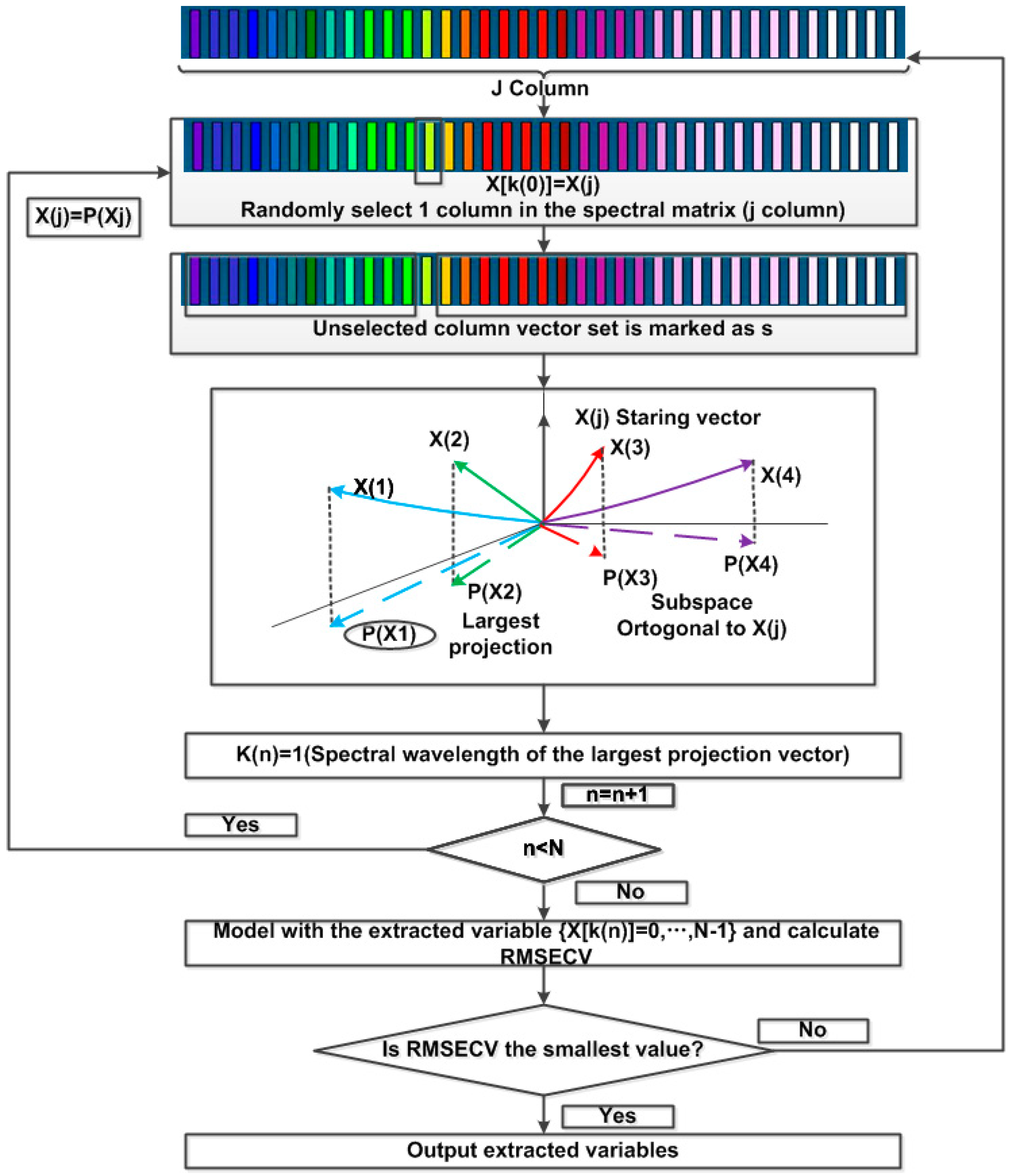
The Successive Projections Algorithm (SPA) was able to fully search for the variable group that contained the minimum redundant information from the spectral information, to minimize the collinearity between variables [36]. At the same time, the number of variables used in modeling could be greatly reduced, and the speed and efficiency of modeling could be improved. As we can see from Figure 4, the SPA was a forward selection method, that is, it started with one wavelength, then incorporated a new one at each iteration, until a specified number N of wavelengths was reached. The SPA employs simple projection operations in a vector space to obtain subsets of variables with small collinearity [37]. Therefore, the SPA method could well solve the collinearity problem, reduce the number of variables, and could be used for the screening of spectral feature wavelengths of large data quantities. The core formula is as follows:
P x j = x j ( x j T x k ( n 1 ) ) x k ( n 1 ) ( x j T x k ( n 1 ) ) 1 ,
where P is the projection operator, all j S , and S is the set of wavelengths not yet selected. K represents the selected wavelength [25].

3.4. Partial Least Squares Regression (PLSR)

Partial least squares regression is a multivariate statistical analysis method that implements the regression modeling of multi-independent variables on multiple independent variables. PLSR is especially more effective when the variables are highly linearly correlated, internally. In addition, PLSR solves the problem that the number of samples is less than the number of variables. The PLSR method is the combination of three components—principal component analysis (PCA), canonical correlation analysis, and multiple linear regression analysis. Both PCA and PLSR attempt to extract the largest amount of information that reflects data variability but PCA considers only one independent variable matrix, whereas PLSR has a “response” matrix and, therefore, has a predictive function [20,38,39]. The PLSR method is implemented by MATLAB R2015b and its extension package.

3.5. Prediction Accuracy

The R 2 , ratio of performance to deviation (RPD), root mean square error (RMSE), and the percentage root mean square error (RMSE%) values were used to access the performance of the soil salt content estimate models. Their calculation formulae were as follows:
R 2 = 1 i = 1 N ( Y i Y ^ i ) 2 i = 1 N ( Y i Y ¯ i ) 2 ,
RPD = SD s RMSE ,
RMSE = i = 1 N ( Y i Y ^ i ) 2 N
RMSE % = RMSE Y p ¯
where N is the sample size, Y i is the measured salt content of soil samples, Y ^ i is the salt content of soil samples predicted by the models, Y ¯ i is the average salt content of soil samples, Y p ¯ is the average of the model predictions, SD s is the standard deviation of measured salt content, and RMSE is the root mean square error of the predicted salt content.
The goodness of the model prediction is reflected by R 2 . The R 2 values indicate the strength of correlation between measured and predicted values [20]. The RPD value provides a basis for standardizing the RMSE. It measures the ratio of percentage deviation to the RMSE and represents the precision of the model. RPD values of less than 1.5 indicate very poor model predictions, between 1.5 and 2.0 indicate poor model predictions, and greater than 2.0 indicate very good model predictions [40]. RMSE is the standard deviation of the residuals (prediction errors). RMSE% refer to the range of the predictions [41].

4. Results

4.1. Salinity Parameters

The basic information of the soil samples was obtained by chemical analysis of the samples. Table 2 shows the range of soil salt content—from 2919.76 mg/kg to 290,857.70 mg/kg. It is known from the calculated Kurtosis value that, in addition to Ca2+, the distribution of other contents is steeper than the normal distribution, and the difference from the normal distribution is large. Except for PH, the skewness of other contents is greater than 0, which indicates that these data are right-biased, compared with the normal distribution, that is, there are more extreme values at the right end of the data. This shows that some soil samples have high salt content.
As shown in Table 3, Spearman rank correlation analysis was conducted on the PH value of the soil, the content of ions in the soil, and the salt content of the soil. From the Spearman rank correlation analysis between soil salinity and other ions, soil salinity mainly existed in the form of sodium, potassium, magnesium, calcium, chloride, and sulfate ions. The most important ions were sodium ions and chloride ions, followed by magnesium ions and sulfate ions. The Spearman rank correlation coefficients between these ions and salt content of the soil was as high as 0.75 or more. According to the correlation analysis between the ions in the soil, the sodium ions mainly combined with the chloride ions to form sodium chloride. The magnesium ions were mainly present in the form of magnesium sulfate, in combination with sulfate ions, followed by the presence of chloride ions in the form of magnesium chloride.
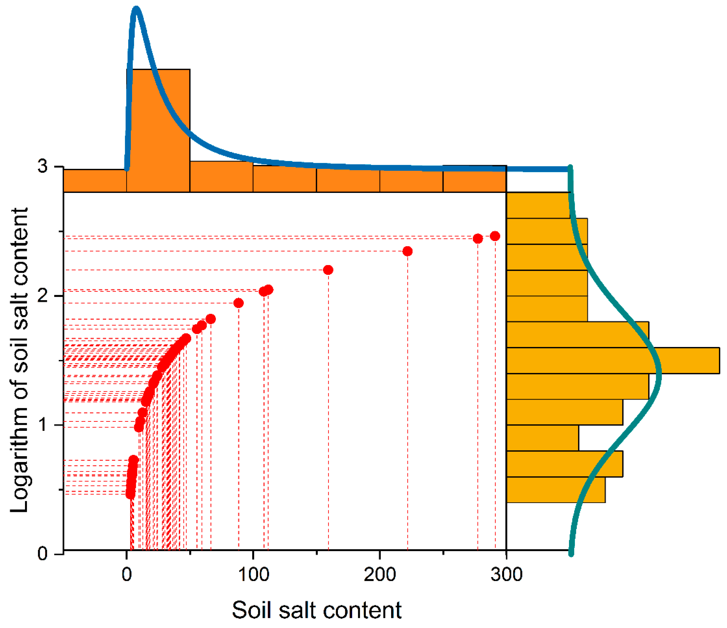
Since the soil salinity parameter data did not belong to the normal distribution, the soil parameter data was converted and the logarithm was obtained to make it normal distributed. As shown in Figure 5. The soil parameter data after the transformation belonged to the normal distribution, and the transformed data was used for modeling analysis.

4.2. Characteristic Analysis of the Varying Spectra

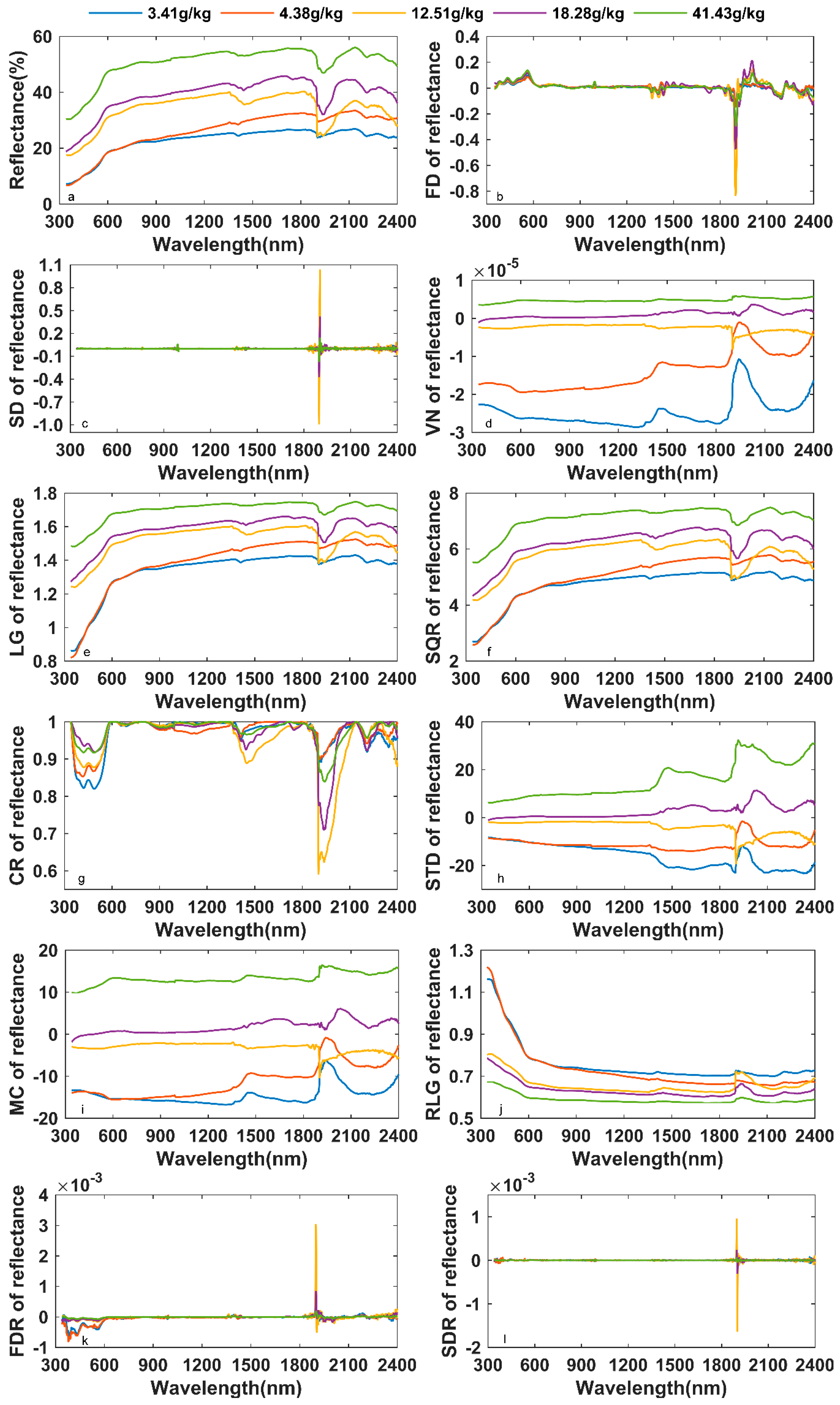
The raw spectra were transformed in 11 ways, and a total of 12 different spectral representations were obtained. Since the spectral was limited by conditions, there was more noise information between 2400 nm to 2500 nm, so in the subsequent analysis and processing, we would discard the spectral range from the raw spectra. As shown in Figure 6, it could be seen from the RS that the higher the salt content of the soil, the larger the spectral reflectance. This is because the spectral measurement time is the salt return period of the soil. The greater the salt content of the soil, the more salt is accumulated on the surface of the soil and the greater is the measured spectral reflectance. Additionally, there was a slight decrease in the RS between 1300 nm and 1500 nm and between 2100 nm and 2300 nm, and there was an absorption band at approximately 1900 nm (Figure 6a). The morphology, variations, and change intervals of logarithm of the reflectance spectra (LG) and square root of the reflectance spectra (SQR) were almost identical to RS, except that the magnitude of some changes was slightly compressed (Figure 6e,f). When the FD was between 300 nm and 600 nm, the higher the soil salinity, the higher was the value of the FD. Moreover, the FD with high soil salinity had a negative value between 1300 nm and 1500 nm and between 2300 nm and 2400 nm, and the FD value with low soil salinity was a positive number. Between 1900 nm and 2100 nm, the value of FD with a high salt content was significantly higher than the value of FD with a low salt content (Figure 6b). Between 300 nm and 600 nm, the vector normalization of the reflectance spectra (VN) and the mean center of the reflectance spectra (MC) of the soil with low salt content showed a slight downward trend, and the soil curve with high salt content showed a straight or slightly rising trend. Their other characteristics are similar to those of RS (Figure 6d,i). The range of CR that distinguished between the most significant changes in soil salt content is 300 nm to 700 nm. The lower the soil salt content, the smaller the CR value (Figure 6g). Between 1500 nm and 1700 nm, the standardization of the reflectance spectra (STD) with low salt content in the soil presented a trough, and the curve with high salinity showed a peak (Figure 6h). The lower the soil salinity, the faster the reciprocal of logarithm of reflectance spectra (RLG) decreases between 300 nm and 600 nm. At the same time, there was a peak in the curve between 1900 nm and 2100 nm (Figure 6j). SD, FDR, and SDR with different salt contents were almost superimposed and difficult to distinguish. Only FDR could distinguish between salt levels from 300 nm to 700 nm (Figure 6c,k,l).

4.3. Feature Band Selected by the SPA Method

For the above-mentioned, 12 different patterns of spectral curves that were transformed and obtained, according to the random classification method, 60 data samples of each set of curves were randomly divided into 40 sets of training data and 20 sets of test data. The 40 training sets were used for the SPA feature band extraction, and the extracted feature bands were then used for modeling. When the SPA feature band selection was performed, the number of selected bands was set to 10. The feature band selected for each spectral transform is shown in Figure 7. The feature bands selected by the SPA method were almost all areas where the bands changed significantly, which indicated that the SPA method could effectively extract the feature bands. The specific location of the feature bands selected by each spectral transform was known from Figure 7. Table 4 shows the wavelengths selected for each spectral form. The feature bands were mainly concentrated in the near-infrared band, especially between 1800 nm and 2400 nm. In addition to SD, the other 10 transforms also selected the feature band between 300 nm and 700 nm. The selected feature bands indicated that the different spectral transformation forms characterized the difference in soil salinity, mainly in the near-infrared band.

4.4. Performance of SPA–PLSR

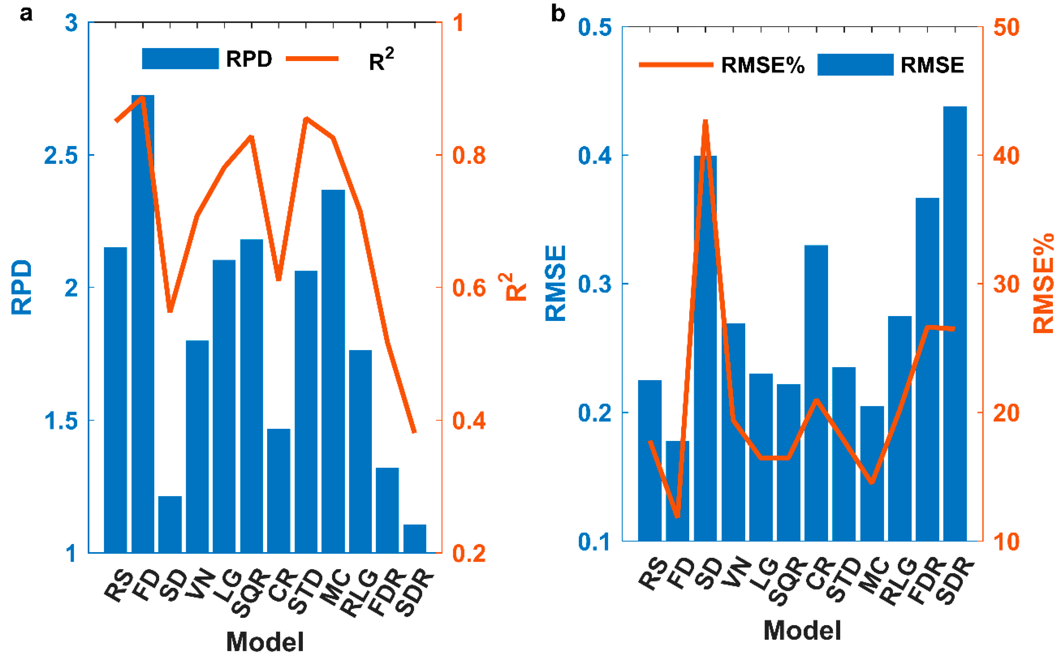
Figure 8 shows the calibration models derived from applying the PLSR model to various transformation methods. By analyzing the R 2 , RPD, RMSE, and RMSE% values that were derived from the calibration models, it was possible to estimate the soil salt content, after selecting the feature bands using the SPA method. It is apparent from Figure 6 that the PLSR models based on different spectral transformation methods yielded significant differences. The best estimates were from RS, FD, SQR, STD, and MC, which produced correlation coefficients higher than 0.8 and RPDs greater than 2. At the same time, lower values of RMSE and RMSE% were obtained. The next-best estimates were from VN, LG, and RLG, which produced R 2 values greater than 0.7, RPDs greater than 1.5, RMSE less than 0.3, and RMSE% less than 20%. The poorest results were from SD, CR, FDR, and SDR; the correlation coefficients obtained by them were low and the RPDs were less than 1.5, which indicated that the models constructed by these four transformations were not suitable for the inversion of the soil salt content. The best estimate was by FD, with an R2 of 0.89, an RPD of 2.72, an RMSE of 0.18, and an RMSE% of 11.81%, followed by STD and RS, with an R2 of 0.86, RPD of 2.06, RMSE of 0.23, and RMSE% of 17.79%, and an R2 of 0.85, RPD of 2.15, RMSE of 0.22, and RMSE% of 17.81%, respectively.
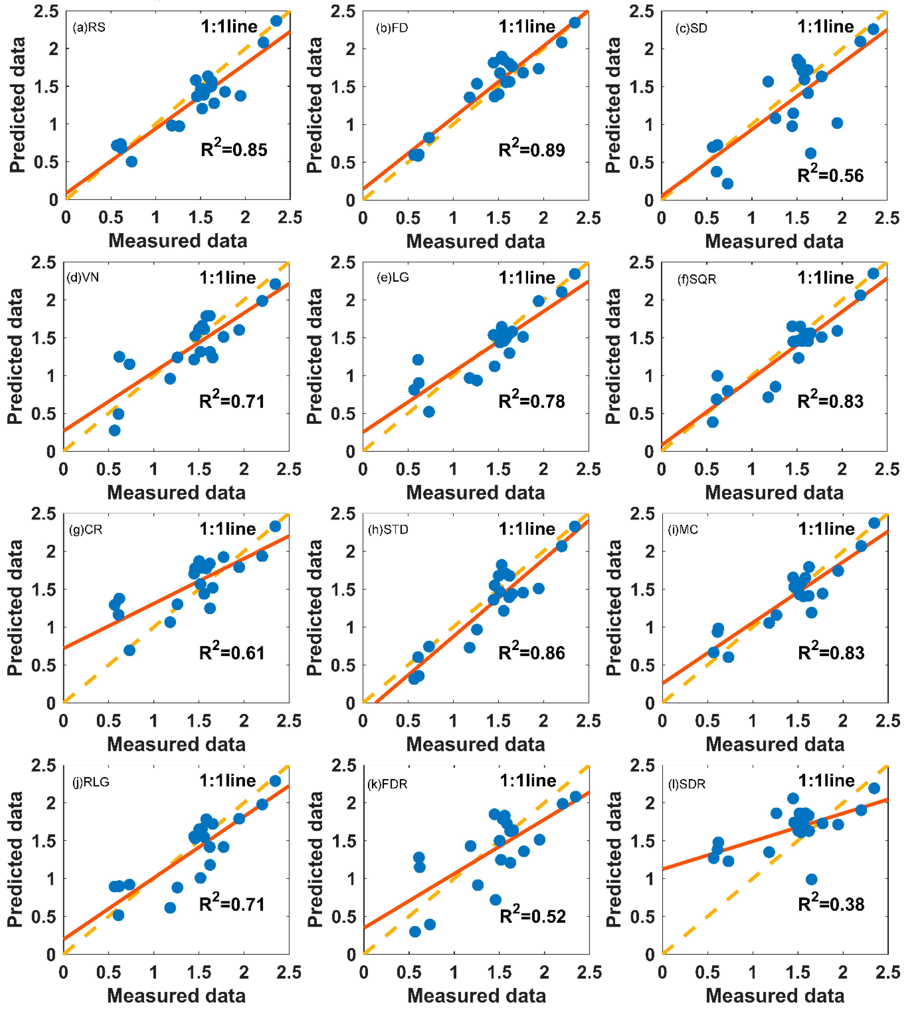
Figure 9 shows a comparison of the estimated results of the twelve models with the measured values. It could be seen that these models produce better estimates of high soil salt content than those with low soil salt content. For the case of low soil salt content, the model is prone to overestimation, such as by CR, SDR, and so on. The lower the salt content of SD, VN, and LG, the more unstable the model estimates. On the one hand, the spectrum is measured in the field, and the external interference conditions are relatively large (prone to the occurrence of dead branches and small gravel), which will affect the spectral information. Especially in the soil spectra with less salt content in the soil, the salt in the original soil has a little effect on the spectral information, and it is difficult to estimate the soils with low salt content, with the external disturbances. On the other hand, this result is the same as that of the results of the Mashimbye et al. [17] and Farifteh et al. [20] studies, which indicated that it is necessary to strengthen the research and screening of spectral information with less soil salt content in subsequent studies.

5. Discussion

5.1. Feature Bands

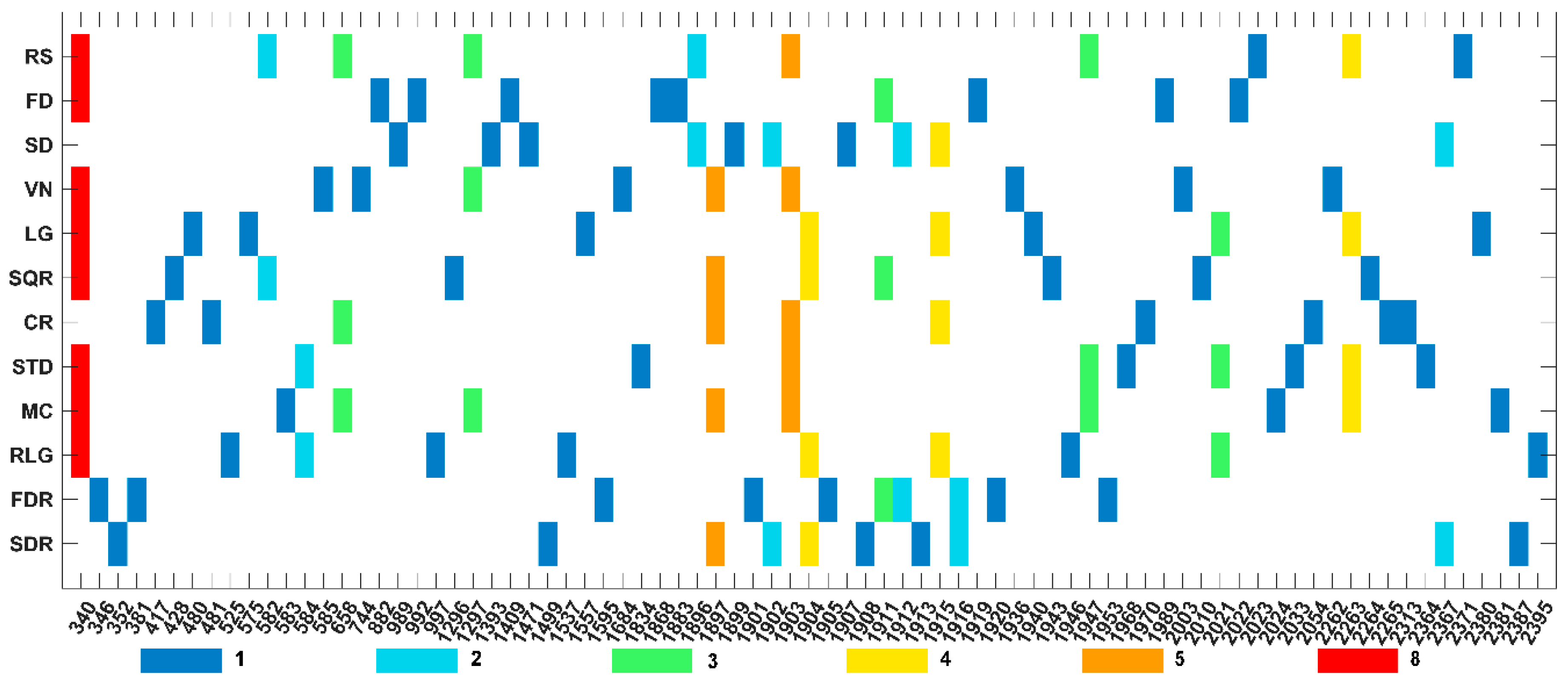
There have been some studies on the relationship between soil salt content and sensitive bands. For example, Abliz et al. [42] used a total of 8 spectral slopes at the wavelength between 365–375 nm, 1435–1465 nm, 1855–1865 nm, 1915–1925 nm, 2085–2095 nm, 2296–2315 nm, 2365–2395 nm, and 2465–2475 nm, which were calculated on the basis of a correlation analysis between soil salt content and soil spectra. Additionally, he used multiple linear regression (MLR) and PLSR to model and estimate soil salt content. Finally, an R 2 result of 0.834 and an RPD result of 2.09 were obtained. The results showed that the selected band range could reflect the feature of soil salt content. Similarly, in the study of Sidike et al. [43], statistical analysis showed that the sensitive bands of soil salinity were 350–436 nm, 516–814 nm, 1445–1506 nm, 1667–1699 nm, 1882–2096 nm, and 2160–2393 nm. In this study, 12 spectral representations were used to select feature bands using the SPA method, and the more repeated bands were 340 nm, 658 nm, 1297 nm, 1897 nm, 1903 nm, 1904 nm, 1911 nm, 1915 nm, 1947 nm, 2021 nm, 2263 nm (Figure 10). The concentrated intervals of these selected bands were mainly 340–481 nm, 525–744 nm, 882–997 nm, 1296–1393 nm, 1409–1684 nm, 1834–1899 nm, 1901–2054 nm, 2262–2395 nm. These selected bands were consistent with the range of bands obtained by previous studies. At the same time, it was more concentrated in the range of 525–744 nm, 1834–1899 nm, and 1901–2054 nm, which indicated that the wavelengths of these three intervals contained more information about the soil salt content.

5.2. The Effect of the SPA Method

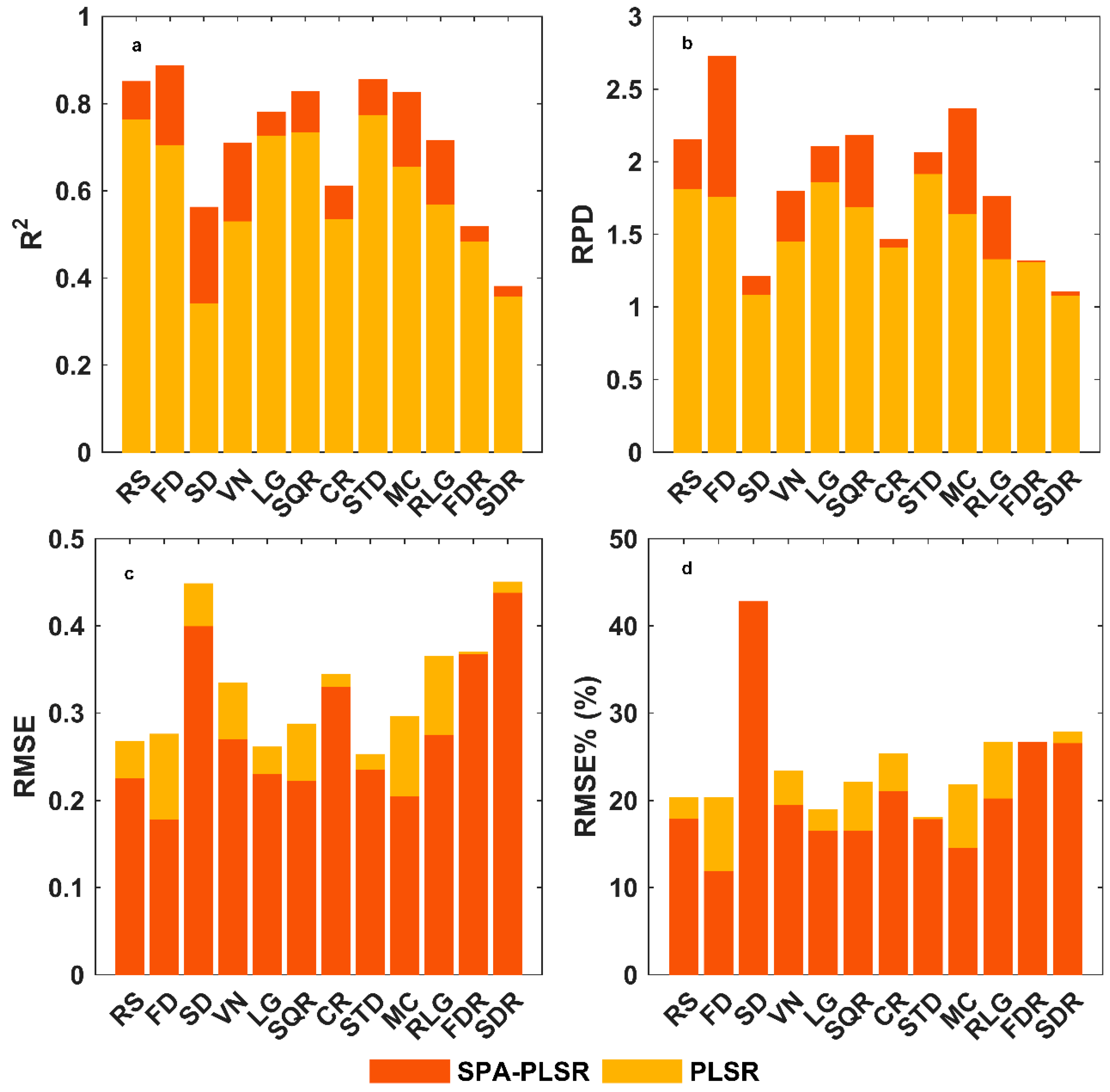
The results of applying the 12 transformed spectra directly to the PLSR modeling are compared with the results of the PLSR modeling, using the feature bands selected by the SPA method. As shown in Figure 11, the results of band modeling after SPA feature extraction are better than those of full-band modeling. Using the SPA–PLSR method, could improve the R2 and RPD of the model and reduce the RMSE and RMSE%, compared to the direct use of the PLSR. The most improved R2 was for SD–SPA–PLSR, which increased from 0.34 to 0.56, an increase of 0.22. The least improvement in R2 was for SDR–SPA–PLSR, which increased from 0.36 to 0.38, an increase of 0.02. The most improved RPD was for FD–SPA–PLSR, which increased from 1.75 to 2.72, an increase of 0.97. The lowest increase in RPD was for FDR–SPA–PLSR, which increased from 1.31 to 1.32, an increase of 0.01. In particular, after RS, FD, LG, SQR, STD, and MC were modelled by SPA–PLSR, the RPD was raised from less than 2 to more than 2, which made these models better estimators of soil salt content, especially the FD–SPA–PLSR model. The largest reduction in RMSE was in the FD–SPA–PLSR model, which decreased from 0.275 to 0.177, a decrease of 0.098. The least RMSE reduction was FDR–SPA–PLSR, which decreased from 0.370 to 0.366, a reduction of 0.004. The largest reduction in RMSE% was in FD–SPA–PLSR, which decreased from 20.33% to 11.81%, a decrease of 8.52%. The least reduction in RMSE% was in STD–SPA–PLSR, which decreased from 18.06% to 17.79%, a decrease of 0.27%.

5.3. The Effect of Selecting the Number of Feature Bands on the Model

When the SPA selection of the feature band was performed, the number of selected bands was set to 10. At the same time, the FD–SPA–PLSR method had obtained the best research results in the previous study. To explore the sensitivity of the model to the number of bands, 2–20 different bands were selected in turn, and then FD–SPA–PLSR modeling estimation was performed to obtain R2, RPD, RMSE, and RMSE% values, corresponding to each band number. As shown in Figure 12, the hollow line represents the estimation results obtained by the RS–PLSR method. When the number of bands was greater than 5, R2 was greater than 0.8, the RPD was greater than 2.0, the RMSE was less than 0.22 and the RMSE% was less than 15%, and, as the number of bands increased, R2 was stable at approximately 0.83, the RPD was stable at approximately 2.4, the RMSE was stable at approximately 0.18 and the RMSE% was stable at approximately 13.5%. The estimated results of the FD–SPA–PLSR model tended to be stable, when the number of selected feature bands was greater than 5.
When the number of selected bands increased from 2, the R2 and RPD increased with an increase in the number of bands and reached the maximum when the number of bands was 10. The RMSE and RMSE% decreased as the number of bands increased and reached the minimum when the number of bands was 10. When the number of bands was greater than 10 and continued to increase, R2, RPD, RMSE, and RMSE% gradually stabilized, which indicated that the bands selected when the number of bands were 10, could well characterize the soil with different salt content. Therefore, the selected bands corresponding to the number of bands from 2 to 10, for this model, are listed (Table 5). According to the previous analysis, the combination of the five wavelengths of 1868 nm, 1883 nm, 1919 nm, 1911 nm, and 2022 nm, could effectively represent the soil salt content information.

5.4. The Availability of the Model

This model is based on the data from proximal-field remote sensing spectral measurements. The data used is point data and, therefore, has a high spatial resolution. At the same time, the data also has a high spectral resolution. It could show more detailed information. However, if the low-distance scale was switched to the remote applications (aerial, satellites), the following factors needed to be considered. First, the proximal-field spectral measurement had less atmospheric impact than the remote sensing image. Therefore, the atmospheric correction and atmospheric correction methods should be considered when switching to remote sensing images. Secondly, the spatial resolution of the existing hyperspectral remote sensing data was “meter” level, so for remote sensing images, each pixel was a mixed pixel, which contained complex surface interference information. For example, the sparse vegetation or the dead branches of the plant on the cultivated field, the moisture content in the soil, and the difference in soil surface roughness caused by the different cultivation environments, these would affect the absorption features of the spectrum and make the spectral curve change. Finally, common hyperspectral image data, such as HyMap (airborne imaging spectrometer), had a spectral resolution between 17–19 nm [6], while the proximal-field spectral resolution was between 3.5 nm and 9 nm, if the proximal scale was converted to an image scale, it also needed to consider the identification and selection of the sensitive bands. Therefore, in subsequent research, the differences between the proximal-field spectral data and remote sensing images, and the effects of these differences should be comprehensively considered, and the results of proximal-field spectral research would be gradually applied to remote sensing images.

6. Conclusions

This study measured the spectra of 60 cultivated lands in the Yellow River Irrigation region of Shizuishan City and collected corresponding soil samples. The relationship between soil spectral information and the corresponding soil salt content was analyzed. First, the spectra were transformed into 11 kinds, and the feature bands were then selected by the SPA feature band selection method. Finally, the regression analysis was performed by PLSR. The research results are as follows.
  • In addition to SD, FDR, and SDR, the other nine kinds of spectra could show different changes in soil salt content to varying degrees.
  • Sensitive bands for soil salt content were 340–481 nm, 525–744 nm, 882–997 nm, 1296–1393 nm, 1409–1684 nm, 1834–1899 nm, 1901–2054 nm, 2262–2395 nm. The most sensitive bands were concentrated at 525–744 nm, 1834–1899 nm, and 1901–2054 nm.
  • Modeling PLSR with feature bands selected by SPA could effectively improve the R 2 and RPD of the model.
  • The FD–SPA–PLSR model had the best estimation results. This model could estimate the soil salt content when the number of bands was greater than 5. The best estimation result could be obtained when the number of bands was 10. Compared with the RS–PLSR model, R2 was increased from 0.76 to 0.89, the RPD was increased from 1.80 to 2.72, the RMSE was decreased from 0.268 to 0.177, and the RMSE% was decreased from 20.27% to 11.81%.
This study explored the applicability of the SPA method for the spectral feature wavelength selection in saline-alkali soils. In future studies, SPA methods could be applied to select the characteristic wavelengths of the saline-alkali soils, and attention should be paid to the salt content inversion of soils with low salinization. At the same time, this study used proximal-field spectral data to provide detailed information. Future research can gradually apply the research results of proximal-field spectroscopy to images, based on a comprehensive consideration of the differences between the proximal-field spectroscopy, and the image scale.

Author Contributions

Data curation, Y.C., M.W., Y.Z. and J.L.; Funding acquisition, Y.C. and J.L.; Methodology, S.W.; Visualization, S.W.; Writing—original draft, S.W.; Writing—review and editing, S.W. and Y.C.

Funding

This research was funded by The Beijing Key Laboratory of Environmental Remote Sensing and Digital City, Ningxia Agriculture, and Animal Husbandry Department East-West Cooperation Project “Study on Remote Sensing Monitoring of Agronomic Improvement of Saline-alkali Land in Yinbei Area”, Ningxia Academy of Agriculture and Forestry Science and Technology Innovation Guide Project (NKYG-18-01).

Conflicts of Interest

The authors declare no conflict of interest.

References

  1. Zhang, D. Application Research of Fractional Derivative in the Remote Sensing Monitoring of Soil Salinization. Ph.D. Thesis, Xinjiang University, Urumqi, China, 2017. [Google Scholar]
  2. Li, T. Study on Typical Saline Region by Remote Sensing Monitoring in the Yellow River Delta. Master’s Thesis, China University of Petroleum (East China), Qingdao, China, 2015. [Google Scholar]
  3. Zhang, T. Evaluate and Analyze land Salinization Pattern, Process and Ecological Effects in the Yellow River Delta: Using Remote Sensing and Ecological Models. Ph.D. Thesis, Fudan University, Shanghai, China, 2011. [Google Scholar]
  4. Hou, C. Research on Remote Sensing Monitoring in the Typical Salt-Affected Zone of the Yellow River Delta Based on BP Neural Net. Master’s Thesis, China University of Petroleum (East China), Qingdao, China, 2010. [Google Scholar]
  5. Bakker, D.M.; Hamilton, G.J.; Hetherington, R.; Spann, C. Salinity dynamics and the potential for improvement of waterlogged and saline land in a Mediterranean climate using permanent raised beds. Soil Tillage Res. 2010, 110, 8–24. [Google Scholar] [CrossRef]
  6. Cécile, G.; Philippe, L.; Guillaume, C. Regional predictions of eight common soil properties and their spatial structures from hyperspectral Vis–NIR data. Geoderma 2012, 189–190, 176–185. [Google Scholar]
  7. Hu, J.; Peng, J.; Zhou, Y.; Xu, D.Y.; Zhao, R.Y.; Jiang, Q.S.; Fu, T.T.; Wang, F.; Shi, Z. Quantitative Estimation of Soil Salinity Using UAV-Borne Hyperspectral and Satellite Multispectral Images. Remote Sens. 2019, 11, 736. [Google Scholar] [CrossRef]
  8. Xu, C.; Zeng, W.; Huang, J.; Wu, J.; Van Leeuwen, W.J. Prediction of Soil Moisture Content and Soil Salt Concentration from Hyperspectral Laboratory and Field Data. Remote Sens. 2016, 8, 42. [Google Scholar] [CrossRef]
  9. Sadro, S.; Gastilbuhl, M.; Melack, J.M. Characterizing patterns of plant distribution in a southern California salt marsh using remotely sensed topographic and hyperspectral data and local tidal fluctuations. Remote Sens. Environ. 2007, 110, 226–239. [Google Scholar] [CrossRef]
  10. Sytar, O.; Brestic, M.; Zivcak, M.; Olsovska, K.; Kovar, M.; Shao, H.; He, X. Applying hyperspectral imaging to explore natural plant diversity towards improving salt stress tolerance. Sci. Total Environ. 2017, 578, 90–99. [Google Scholar] [CrossRef] [PubMed] [Green Version]
  11. Nawar, S.; Buddenbaum, H.; Hill, J. Estimation of soil salinity using three quantitative methods based on visible and near-infrared reflectance spectroscopy: A case study from Egypt. Arab. J. Geosci. 2015, 8, 5127–5140. [Google Scholar] [CrossRef]
  12. Scudiero, E.; Skaggs, T.H.; Corwin, D.L. Regional-scale soil salinity assessment using Landsat ETM+ canopy reflectance. Remote Sens. Environ. 2015, 169, 335–343. [Google Scholar] [CrossRef]
  13. Bouaziz, M.; Matschullat, J.; Gloaguen, R. Improved remote sensing detection of soil salinity from a semi-arid climate in Northeast Brazil. C. R. Geosci. 2011, 343, 795–803. [Google Scholar] [CrossRef]
  14. Lobell, D.B.; Lesch, S.M.; Corwin, D.L.; Ulmer, M.G.; Anderson, K.A.; Potts, D.J.; Doolittle, J.A.; Matos, M.R.; Baltes, M.J. Regional-scale Assessment of Soil Salinity in the Red River Valley Using Multi-year MODIS EVI and NDVI. J. Environ. Qual. 2010, 39, 35–41. [Google Scholar] [CrossRef]
  15. Yan, L.I.; Shi, Z.; Cifang, W.U.; Hongyi, L.I.; Feng, L.I. Improved Prediction and Reduction of Sampling Density for Soil Salinity by Different Geostatistical Methods. Agric. Sci. China 2007, 6, 832–841. [Google Scholar]
  16. Dehaan, R.L.; Taylor, G.R. Field-derived spectra of salinized soils and vegetation as indicators of irrigation-induced soil salinization. Remote Sens. Environ. 2002, 80, 406–417. [Google Scholar] [CrossRef]
  17. Mashimbye, Z.E.; Cho, M.A.; Nell, J.P.; De Clercq, W.P.; Van Niekerk, A.; Turner, D.P. Model-Based Integrated Methods for Quantitative Estimation of Soil Salinity from Hyperspectral Remote Sensing Data: A Case Study of Selected South African Soils. Pedosphere 2012, 22, 640–649. [Google Scholar] [CrossRef]
  18. Peng, J.; Wang, J.Q.; Xiang, H.Y.; Teng, H.F.; Liu, W.Y.; Chi, C.M.; Niu, J.L.; Guo, j.; Shi, Z. Comparative Study on Hyperspectral Inversion Accuracy of Soil Salt Content and Electrical Conductivity. Spectrosc. Spectr. Anal. 2014, 34, 510. [Google Scholar]
  19. Zhang, T.; Zeng, S.; Gao, Y.; Ouyang, Z.; Li, B.; Fang, C.; Zhao, B. Using hyperspectral vegetation indices as a proxy to monitor soil salinity. Ecol. Indic. 2011, 11, 1552–1562. [Google Scholar] [CrossRef]
  20. Farifteh, J.; Der Meer, F.D.; Atzberger, C.; Carranza, E.J. Quantitative analysis of salt-affected soil reflectance spectra: A comparison of two adaptive methods (PLSR and ANN). Remote Sens. Environ. 2007, 110, 59–78. [Google Scholar] [CrossRef]
  21. Wang, J.; Qin, L.; Wu, G. Application of Successive Projections Algorithm in Quantitative Analysis of Winter Wheat Hyper-spectral Variables. Electron. R D 2011, 38, 13–15. [Google Scholar]
  22. Cheng, Z.; Zhang, L.Q.; Liu, H.Y.; Zhu, A.S. Successive projections algorithm and its application to selecting the wheat near-infrared spectral variables. Spectrosc. Spectr. Anal. 2010, 30, 949. [Google Scholar]
  23. Kumar, S.; Gautam, G. Hyperspectral remote sensing data derived spectral indices in characterizing salt-affected soils: A case study of Indo-Gangetic plains of India. Environ. Earth Sci. 2015, 73, 3299–3308. [Google Scholar] [CrossRef]
  24. Allbed, A.; Kumar, L.; Aldakheel, Y.Y. Assessing soil salinity using soil salinity and vegetation indices derived from IKONOS high-spatial resolution imageries: Applications in a date palm dominated region. Geoderma 2014, 230–231, 1–8. [Google Scholar] [CrossRef]
  25. De Araujo, M.C.; Saldanha, T.C.; Galvao, R.K.; Yoneyama, T.; Chame, H.C.; Visani, V. The successive projections algorithm for variable selection in spectroscopic multicomponent analysis. Chemom. Intell. Lab. Syst. 2001, 57, 65–73. [Google Scholar] [CrossRef]
  26. Inácio, M.R.C.; de Moura, M.d.V.; de Lima, K.M.G. Classification and determination of total protein in milk powder using near infrared reflectance spectrometry and the successive projections algorithm for variable selection. Vib. Spectrosc. 2011, 57, 342–345. [Google Scholar] [CrossRef]
  27. Goudarzi, N.; Goodarzi, M. Application of successive projections algorithm (SPA) as a variable selection in a QSPR study to predict the octanol/water partition coefficients (Kow) of some halogenated organic compounds. Anal. Methods 2010, 2, 758–764. [Google Scholar] [CrossRef]
  28. Liu, F.; He, Y. Application of successive projections algorithm for variable selection to determine organic acids of plum vinegar. Food Chem. 2009, 115, 1430–1436. [Google Scholar] [CrossRef]
  29. Tang, R.; Chen, X.; Li, C. Detection of Nitrogen Content in Rubber Leaves Using Near-Infrared (NIR) Spectroscopy with Correlation-Based Successive Projections Algorithm (SPA). Appl. Spectrosc. 2018, 72, 740–749. [Google Scholar] [CrossRef] [PubMed]
  30. Zhu, H.; Chu, B.; Zhang, C.; Liu, F.; Jiang, L.; He, Y. Hyperspectral Imaging for Presymptomatic Detection of Tobacco Disease with Successive Projections Algorithm and Machine-learning Classifiers. Sci. Rep. 2017, 7, 4125. [Google Scholar] [CrossRef] [Green Version]
  31. Liu, Y.; Zhou, S.; Liu, W.; Yang, X.; Luo, J. Least-squares support vector machine and successive projection algorithm for quantitative analysis of cotton-polyester textile by near infrared spectroscopy. J. Near Infrared Spectrosc. 2018, 26, 34–43. [Google Scholar] [CrossRef]
  32. Liu, X.Q.; Yang, J.G.; Cui, Y.X.; Gao, Y.; Fan, L.Q.; Shang, H.Y.; Ji, L.D.; Du, Y.X. The improvement strategy of saline-alkali land in Shizuishan City. Ningxia Agric. Sci. Technol. 2010, 6, 63–66. [Google Scholar]
  33. Re, E.D. Digital Processing of Signals: Theory and Practice; IEEE Transactions on Acoustics, Speech, and Signal Processing; Wiley: New York, NY, USA, 1985; Volume 33, pp. 1062–1063. [Google Scholar]
  34. Steinier, J.; Termonia, Y.; Deltour, J. Smoothing and Differentiation of Data by Simplified Least Squares Procedures. Anal. Chem. 1964, 36, 1627–1639. [Google Scholar] [CrossRef] [PubMed]
  35. He, Y.; Liu, F.; Li, X.L.; Shao, Y.N. Spectroscopy and Imaging Technology in Agriculture; Science Press: Beijing, China, 2016; pp. 106–107. [Google Scholar]
  36. Galvao, R.K.; De Araujo, M.C.; Fragoso, W.D.; Silva, E.C.; Jose, G.E.; Soares, S.F.; Paiva, H.M. A variable elimination method to improve the parsimony of MLR models using the successive projections algorithm. Chemom. Intell. Lab. Syst. 2008, 92, 83–91. [Google Scholar] [CrossRef]
  37. Xiaobo, Z.; Jiewen, Z.; Hanpin, M.; Jiyong, S.; Xiaopin, Y.; Yanxiao, L. Genetic Algorithm Interval Partial Least Squares Regression Combined Successive Projections Algorithm for Variable Selection in Near-Infrared Quantitative Analysis of Pigment in Cucumber Leaves. Appl. Spectrosc. 2010, 64, 786–794. [Google Scholar] [CrossRef]
  38. Nawar, S.; Buddenbaum, H.; Hill, J.; Kozak, J.; Mouazen, A.M. Estimating the soil clay content and organic matter by means of different calibration methods of vis-NIR diffuse reflectance spectroscopy. Soil Tillage Res. 2016, 155, 510–522. [Google Scholar] [CrossRef]
  39. Martens, H.; Anderssen, E.; Flatberg, A.; Gidskehaug, L.; Hoy, M.; Westad, F.; Thybo, A.K.; Martens, M. Regression of a data matrix on descriptors of both its rows and of its columns via latent variables: L-PLSR. Comput. Stat. Data Anal. 2005, 48, 103–123. [Google Scholar] [CrossRef]
  40. Rossel, V. Robust modelling of soil diffuse reflectance spectra by bagging-partial least squares regression. J. Near Infrared Spectrosc. 2007, 15, 39–47. [Google Scholar] [CrossRef]
  41. Malavolti, M.; Battistini, N.; Bedogni, G.; Poli, M.; Mussi, C.; Salvioli, G. Cross-calibration of eight-polar bioelectrical impedance analysis versus dual-energy X-ray absorptiometry for the assessment of total and appendicular body composition in healthy subjects aged 21–82 years. Ann. Hum. Biol. 2003, 30, 380–391. [Google Scholar] [CrossRef]
  42. Abliz, A.; Tiyip, T.; Ding, J.; Sawut, M.; Hou, Y.; Nurmemet, I. Estimating Soil Salt Content in the Keriya Oasis Using Hyperspectral Slope Index. Nat. Environ. Pollut. Technol. 2017, 16, 141–146. [Google Scholar]
  43. Sidike, A.; Zhao, S.; Wen, Y. Estimating soil salinity in Pingluo County of China using QuickBird data and soil reflectance spectra. Int. J. Appl. Earth Obs. Geoinf. 2014, 26, 156–175. [Google Scholar] [CrossRef]
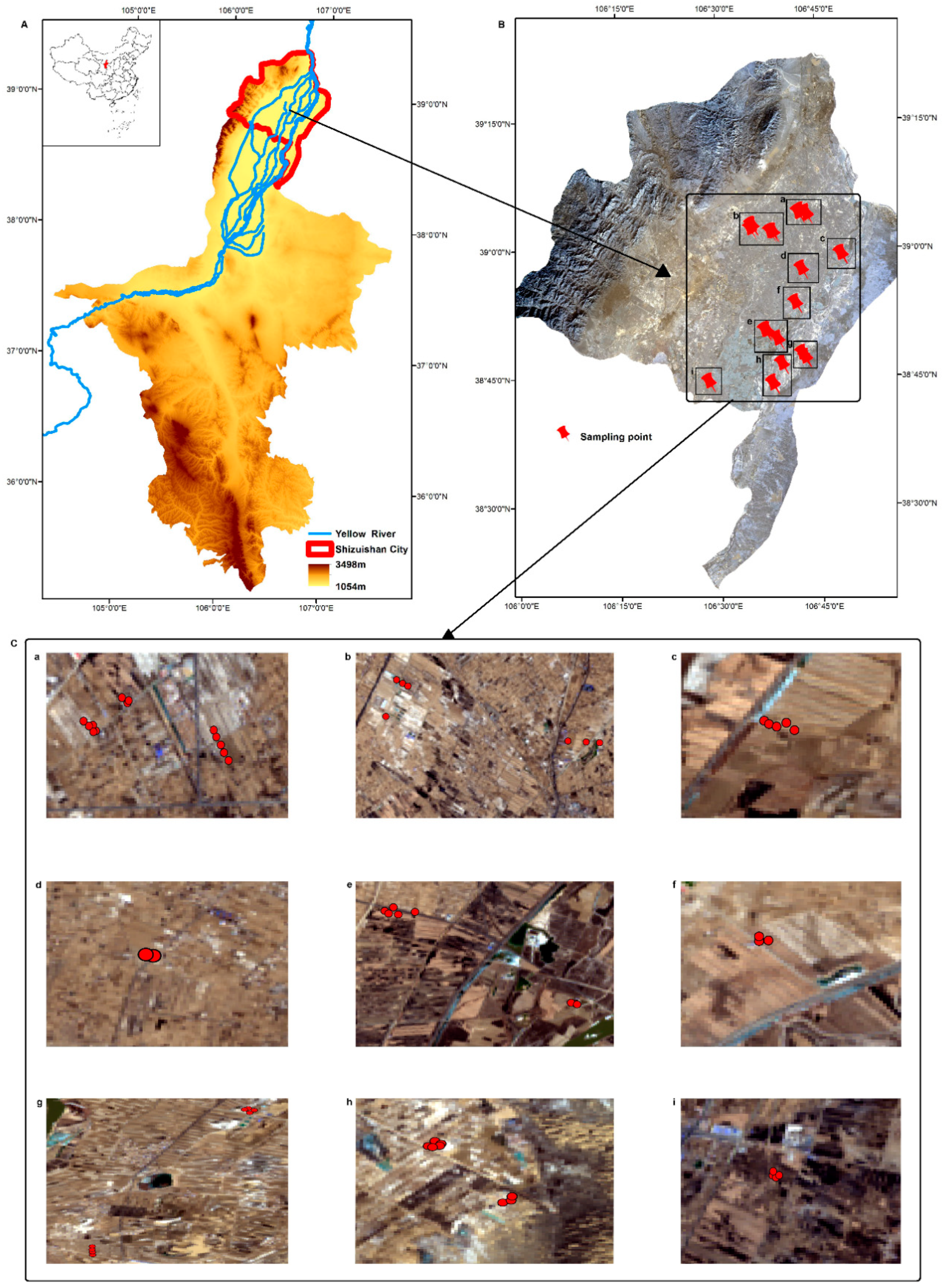
Figure 1. Study area and sampling location. (A) A Digital Elevation Model (DEM) diagram of the Ningxia Hui Autonomous Region, made using the original elevation data of the Shuttle Radar Topography Mission (SRTM) DEM 90-meter resolution data product. (B) The sampling location around the Yellow River Irrigation region in Shizuishan City, made from the Landsat 8 data of April 2018. (ai) in B correspond one-to-one with (a–i) in (C) and show the specific position and surrounding conditions of the sampling point.
Remotesensing 11 00967 g001
Figure 2. Field data measurement. (a) The steps of the field data collection; (b1) the spectrum measurement photo, (b2) the record of the collected data, and (b3) the saline-alkali photo of one of the data collection sites. The white matter on the land-like snow was the salt on the surface of the land, indicating that the salinization of this cultivated land was very serious.
Remotesensing 11 00967 g002
Figure 3. Method flow chart. (a) Data preprocessing; (b) modeling; and (c) analysis.
Remotesensing 11 00967 g003
Figure 4. Successive Projections Algorithm (SPA) schematic; the SPA includes two phases. At first, the algorithm builds candidate subsets of variables on the basis of a collinearity minimization criterion. Such subsets are built according to a sequence of vector projection operations applied to the columns of the matrix of available predictor data. In the second phase, the best candidate subset is chosen, based on Root Mean Squares Error Cross Validation (RMSECV) obtained in a validation set [27].
Remotesensing 11 00967 g004
Figure 5. Soil salt content parameter data distribution. The horizontal axis represents soil salt content. The vertical axis represents the logarithm of soil salt content. Each point represents every piece of data. The histogram shows the distribution of the data. It indicates that the soil salt content parameter data is in a normal distribution, after the logarithmic transformation.
Remotesensing 11 00967 g005
Figure 6. Spectral transformation curve (a) the raw reflectance spectra (RS), (b) the first derivative of the reflectance spectra (FD), (c) the second derivative of the reflectance spectra (SD), (d) the vector normalization of the reflectance spectra (VN), (e) the logarithm of the reflectance spectra (LG), (f) the square root of the reflectance spectra (SQR), (g) the continuum removal of the reflectance spectra (CR), (h) the standardization of the reflectance spectra (STD), (i) the mean center of the reflectance spectra (MC), (j) the reciprocal of logarithm of reflectance spectra (RLG), (k) the first derivative of reciprocal of the reflectance spectra (FDR), and (l) the second derivative of the reciprocal of the reflectance spectra (SDR).
Remotesensing 11 00967 g006
Figure 7. The selected bands of different transformation (a) the raw reflectance spectra (RS), (b) the first derivative of the reflectance spectra (FD), (c) the second derivative of the reflectance spectra (SD), (d) the vector normalization of the reflectance spectra (VN), (e) the logarithm of the reflectance spectra (LG), (f) the square root of the reflectance spectra (SQR), (g) the continuum removal of the reflectance spectra (CR), (h) the standardization of the reflectance spectra (STD), (i) the mean center of the reflectance spectra (MC), (j) the reciprocal of logarithmic of reflectance spectra (RLG), (k) the first derivative of reciprocal of the reflectance spectra (FDR), and (l) the second derivative of the reciprocal of the reflectance spectra (SDR).
Remotesensing 11 00967 g007
Figure 8. Model estimate results. Model estimation results of the SPA–Partial Least Squares Regression (PLSR) based on different spectral forms. (a) Represents the ratio of performance to deviation (RPD) and R 2 of the model estimation result, and (b) represents the root mean square error (RMSE) and RMSE% of the model estimation result.
Remotesensing 11 00967 g008
Figure 9. SPA–PLSR estimate results. (a) RS–SPA–PLSR estimate results, (b) FD–SPA–PLSR estimate results, (c) SD–SPA–PLSR estimate results, (d) VN–SPA–PLSR estimate results, (e) LG–SPA–PLSR estimate results, (f) SQR–SPA–PLSR estimate results, (g) CR–SPA–PLSR estimate results, (h) STD–SPA–PLSR estimate results, (i) MC–SPA–PLSR estimate results, (j) RLG–SPA–PLSR estimate results, (k) FDR–SPA–PLSR estimate results, and (l) SDR–SPA–PLSR estimate results.
Remotesensing 11 00967 g009
Figure 10. Concentrated map of selected bands of the different spectral forms. The horizontal axis represents the wavelength of the selected band, and the vertical axis represents the 12 spectral forms. The different colors indicate the number of times each wavelength was selected. From left to right, the wavelength selected for each form can be known. From top to bottom, which form is selected for each wavelength can be seen.
Remotesensing 11 00967 g010
Figure 11. Comparison of the SPA–PLSR and PLSR results. (a) Shows the change in R2; (b) shows the change in RPD; (c) shows the change in RMSE; and (d) shows the change in RMSE%. The red bar chart represents the results of the SPA–PLSR model, the yellow bar chart represents the results of the PLSR model.
Remotesensing 11 00967 g011
Figure 12. Sensitivity analysis. (a) The hollow line in the figure shows the result obtained by the RS–PLSR method; the black line indicates R 2 , and the red line indicates RPD. (b) The hollow line in the figure shows the result obtained by the RS–PLSR method; the black line indicates RMSE and the red line indicates RMSE%.
Remotesensing 11 00967 g012
Table 1. Spectral transformation method.
NameMethod or FormulaAbbreviation
First derivative [34]Savitzky–Golay methodFD
Second Derivative [34]Savitzky–Golay methodSD
Vector normalization [35] x vn = x x ¯ i = 1 p x i 2 VN
Logarithm x lg = log 10 ( x i ) LG
Square root x sqrt = x i SQR
Continuum removal X h ( λ ) = X cr ( λ ) X ( λ ) CR
Standardization [35] x scal = x X ¯ S STD
Mean centering [35] x mcenter = x X ¯ MC
Reciprocal of logarithmic x 1 / lg = 1 / log 10 ( x i ) RLG
First derivative of the reciprocal [34]Savitzky–Golay methodFDR
Second derivative of the reciprocal [34]Savitzky–Golay methodSDR
Table 2. Descriptive statistics of the soil.
PHSalt ContentNa+K+Mg2+Ca2+ClNO3−SO42−CO32−HCO3−
Unit1mg/kgmg/kgmg/kgmg/kgmg/kgmg/kgmg/kgmg/kgmg/kgmg/kg
Min7.532919.76327.7128.4043.75187.15178.3922.9414.640.00145.69
Max9.98290,857.7087,551.62370.247508.089416.3589,678.662701.8698,199.803133.70891.37
Mean8.5643,827.4012,840.01101.251263.773291.6012,103.64502.7813,715.9863.81321.44
Kurtosis0.209.437.864.997.37−0.668.552.8810.7956.772.79
Skewness−0.113.022.771.942.700.532.881.693.277.531.60
SD0.4958,950.6618,656.0364.341621.672269.1718,473.84584.6920,157.66407.23150.24
Table 3. Spearman rank correlation coefficients between measured soil variables.
PHSalt ContentNa+K+Mg2+Ca2+ClNO3−SO42−CO32−HCO3
PH1.000
Salt content0.3341.000
Na+0.4510.9291.000
K+0.0470.5730.5251.000
Mg2+0.1260.7730.6690.5801.000
Ca2+−0.0200.6470.4530.5100.8001.000
Cl0.3650.9360.9450.4700.7410.4741.000
NO3−−0.0410.3020.2860.3120.260−0.0050.3811.000
SO42−0.1310.8360.6620.5300.7670.7520.7070.1881.000
CO32−0.1770.2660.286−0.0190.096−0.0230.289−0.0280.0971.000
HCO30.1950.2250.2320.0010.1480.1240.221−0.0680.2250.4691.000
Table 4. Feature bands selected by the SPA method.
Spectral TransformationFeature Bands (nm)
RS3405826581297189619031947202322632371
FD3408829921409186818831911191919892022
SD989139314711896189919021907191219152367
VN3405857441297168418971903193620032262
LG3404805751557190419151940202122632380
SQR3404285821296189719041911194320102264
CR4174816581897190319151970205422652313
STD34058418341903194719682021203322632364
MC3405836581297189719031947202422632381
RLG340525584997153719041915194620212395
FDR34638115951901190519111912191619201953
SDR352149918971902190419081913191623672387
Table 5. Bands selected by the number of bands of 2–10, selected on the basis of the FD–SPA–PLSR model.
Number of Bands2345678910
The selected feature bands186818681868186818681868186818681868
188318831883188318831883188318831883
19191919191919191919191919191919
1911191119111911191119111911
202220222022202220222022
14091409140914091409
992992992992
340340340
19891989
882
R20.7000.7160.7720.8170.8220.8330.8410.8450.876
RPD1.7981.8391.9242.2712.3102.3722.3922.4012.763