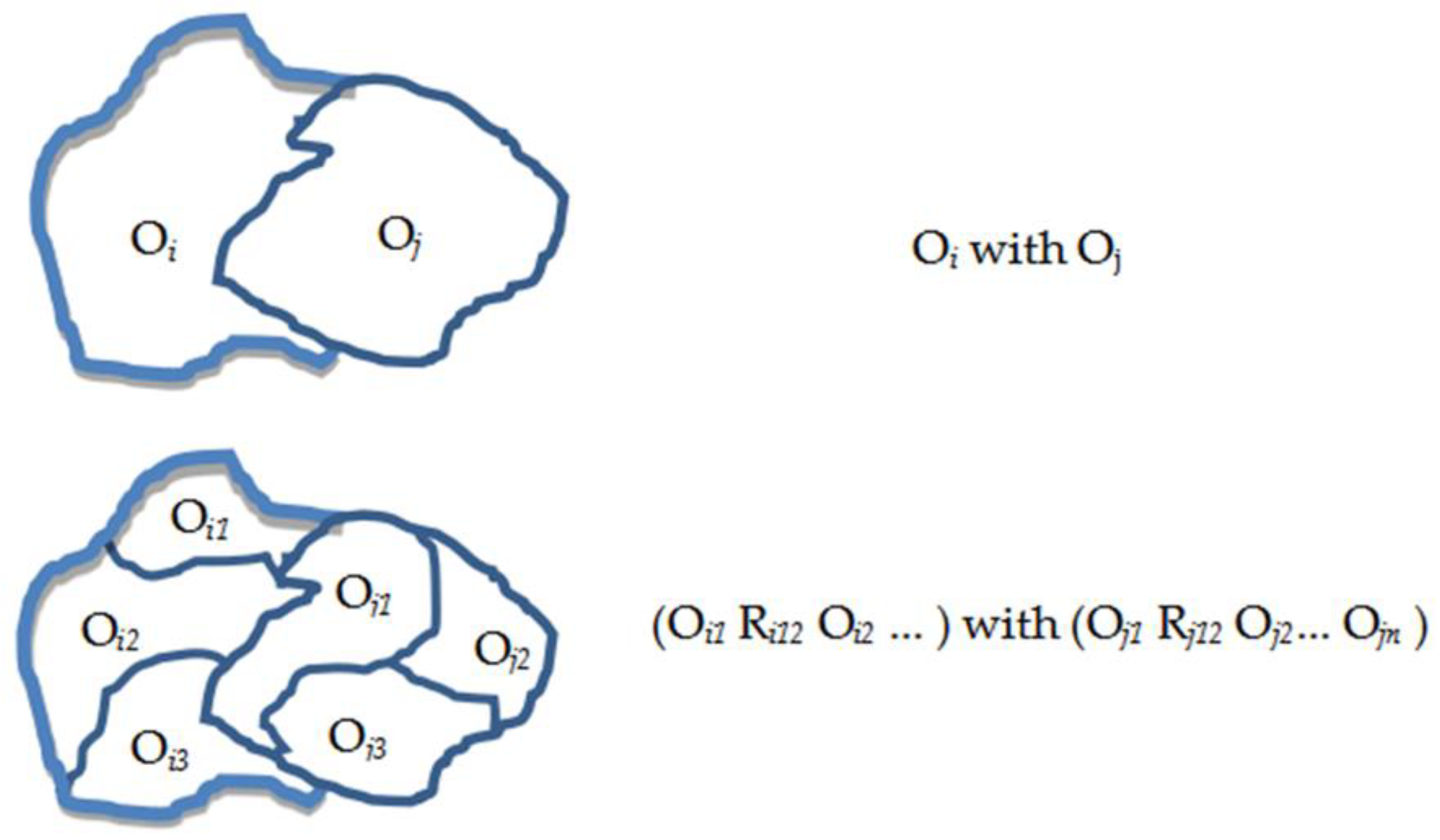
Figure 1.
Multi-spatial scale semantic segmentation and image caption. It shows a two-scale hierarchy of one image. An image contains many large-scale objects, each large-scale object contains many small-scale objects, and there are spatial relationships between objects of the same scale. Our strategy of captioning is to describe both information of scale and spatial relationship contained in an image as completely as possible.
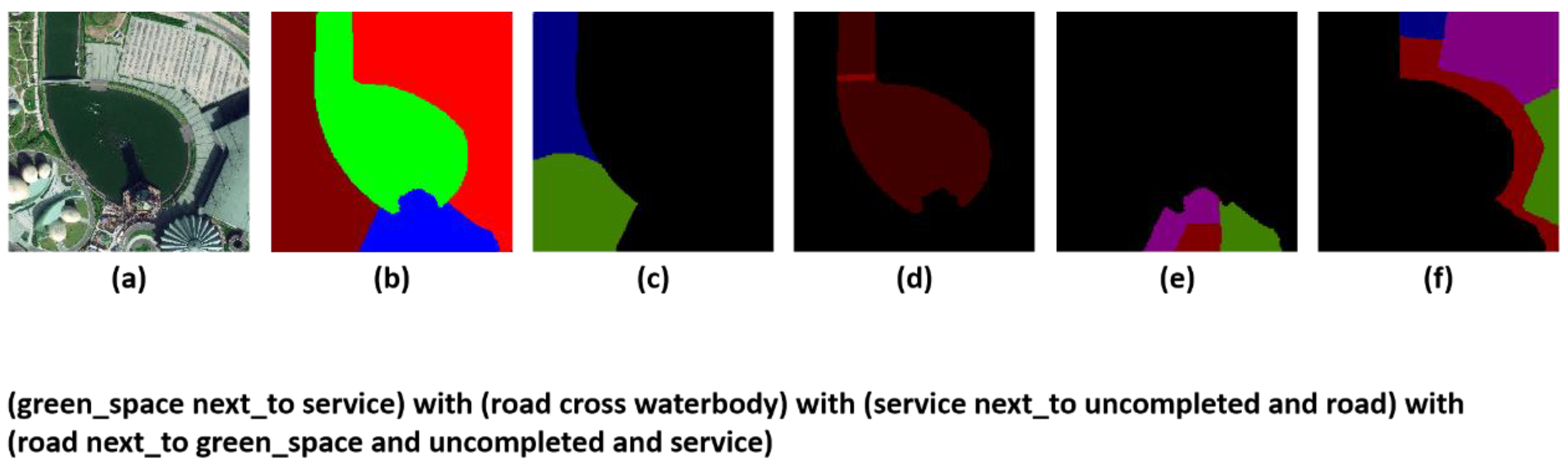
Figure 2.
Sample with complex scenes. It shows an image with more complex scenes that contain four large-scale objects. (a) is the input image; (b) is the large-scale segmentation map of (a); (c–f) are the small-scale objects contained in each large-scale object. (c) corresponds to the clause “green_space next_to service,” (d) to the clause “road cross waterbody,” (e) to the clause “service next_to uncompleted and road,” and (f) to the clause “road next_to green_space and uncompleted and service.”.
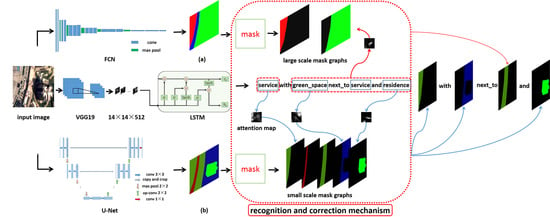
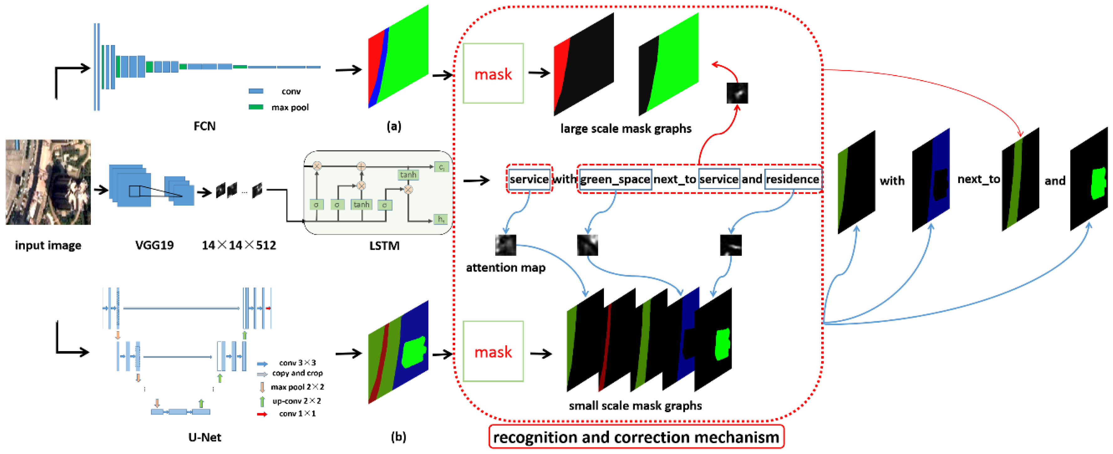
Figure 3.
Network structure. It shows the overall network structure of the MSRIN. In our network, one remote sensing image is input into three branch networks. (
a) is the large-scale segmentation map of the FCN output, (
b) is the small-scale segmentation map of the U-Net output, and they are masked to obtain the location and boundaries of remote sensing objects. The LSTM outputs image captions and attention areas. The process of identification and correction is given in
Section 3.3. The multi-scale objects recognition and correction mechanism attaches the object (the mask graphs from U-Net) to nount through the weight matrix at time step
t.
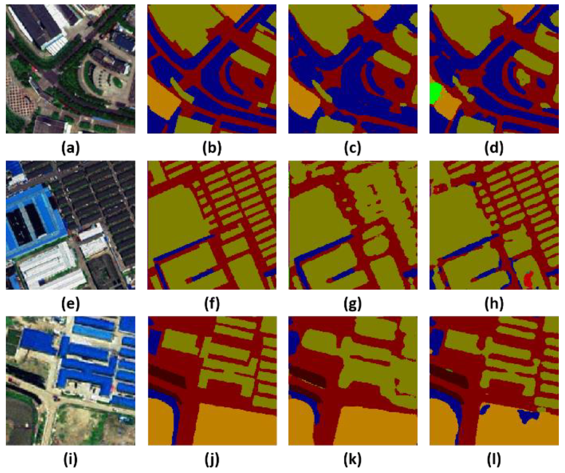
Figure 4.
Segmentation effect of FCN and U-Net. It shows three examples of FCN and U-Net segmentation effect comparison. (a,e,i) are the input images. (b,f,j) are corresponding ground truth of the images. (c,g,k) are segmentation maps of FCN. (d,h,l) are segmentation maps of U-Net. It was found that FCN performed better at segmenting large objects, while smaller objects were easier to aggregate into blocks, so FCN was more suitable for large-scale segmentation. U-Net worked well when smaller objects were segmented but tended to misclassify some small fragments of the large-scale objects when it was being segmented, so U-Net was more suitable for small-scale segmentation.
Figure 5.
Attention weight matrix error. It shows mismatches between nouns in the caption and objects in the image. (a) is the input image; (b–d) are the attention maps for generating “green_space,” “service,” and “waterbody,” respectively; (e) is a small-scale segmentation map of (a); (f–h) are overlaid maps of (b–d), respectively, with (e). As shown in the figure, the attention area of the first generated noun “green_space” corresponds to the object “waterbody” in the image, which resulted in mismatch. Of the three nouns contained in the generated image caption, only the third noun matched the right object.
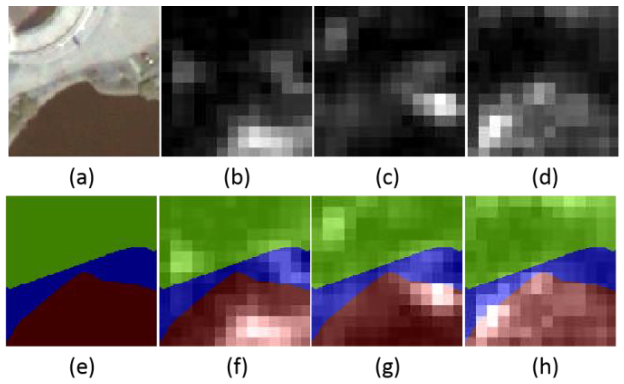
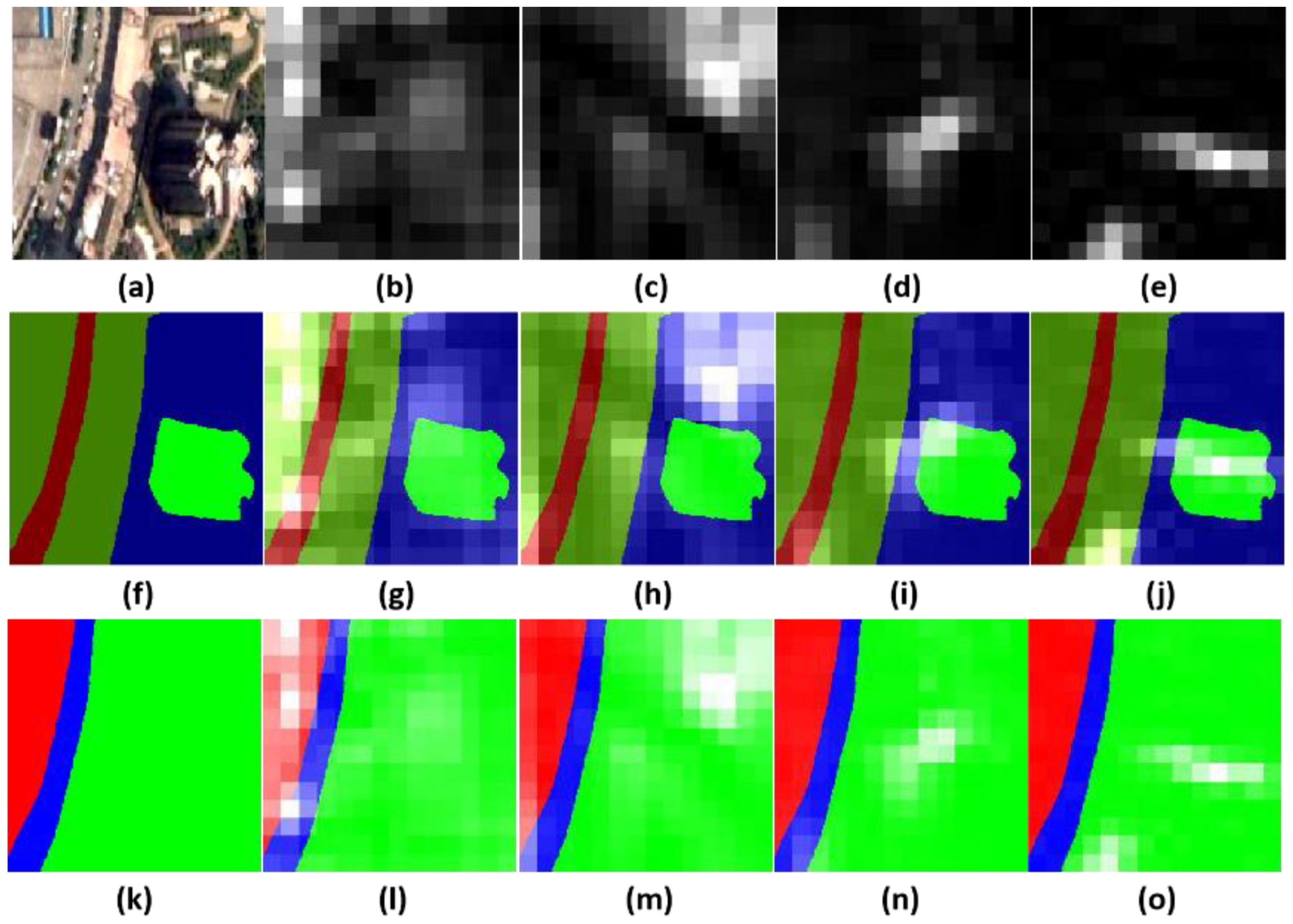
Figure 6.
Remote sensing object recognition and correction. It shows the process of multi-scale remote sensing object recognition. (a) is the input image; (b–e) are the attention maps for generating “service,” “green_space,” “service,” and “residence,” respectively; (f) is a small-scale segmentation map of (a); (g–j) are overlaid maps of (b–e), respectively, with (f); (k) is a large-scale segmentation map of (a); (l–o) are overlaid maps of (b–e), respectively, with (k). As shown in (I,n), when generating the second “service,” the spatial location of attention weights is incorrect at the small scale, but it is correct at the large scale.
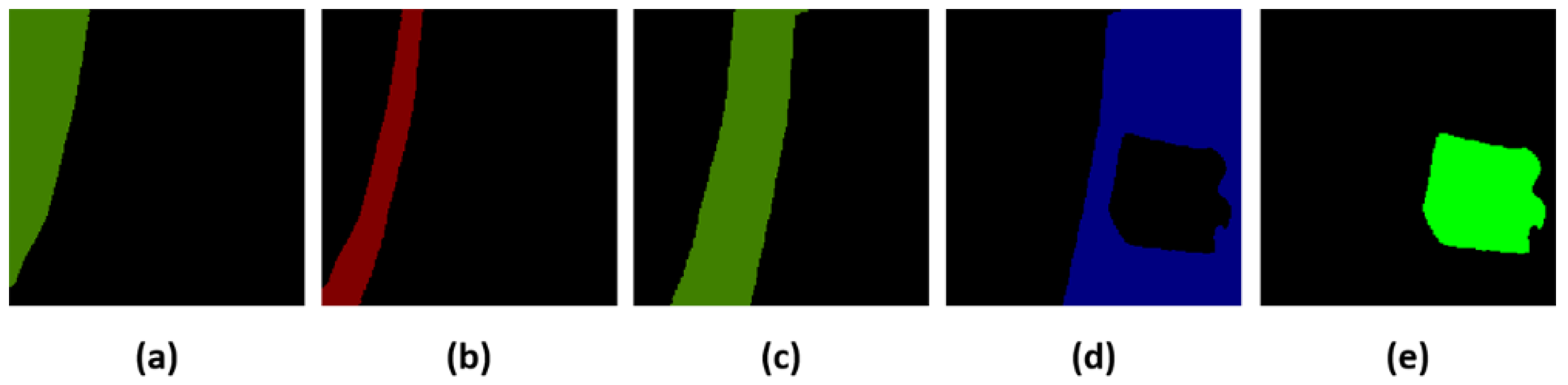
Figure 7.
Small-scale objects. It shows the small-scale objects of the image. (a) is service_0 (in order to distinguish between different objects of the same class, we number each object); (b) is road_0; (c) is service_1; (d) is green_space _0; and (e) is residence_0.
Figure 7.
Small-scale objects. It shows the small-scale objects of the image. (a) is service_0 (in order to distinguish between different objects of the same class, we number each object); (b) is road_0; (c) is service_1; (d) is green_space _0; and (e) is residence_0.
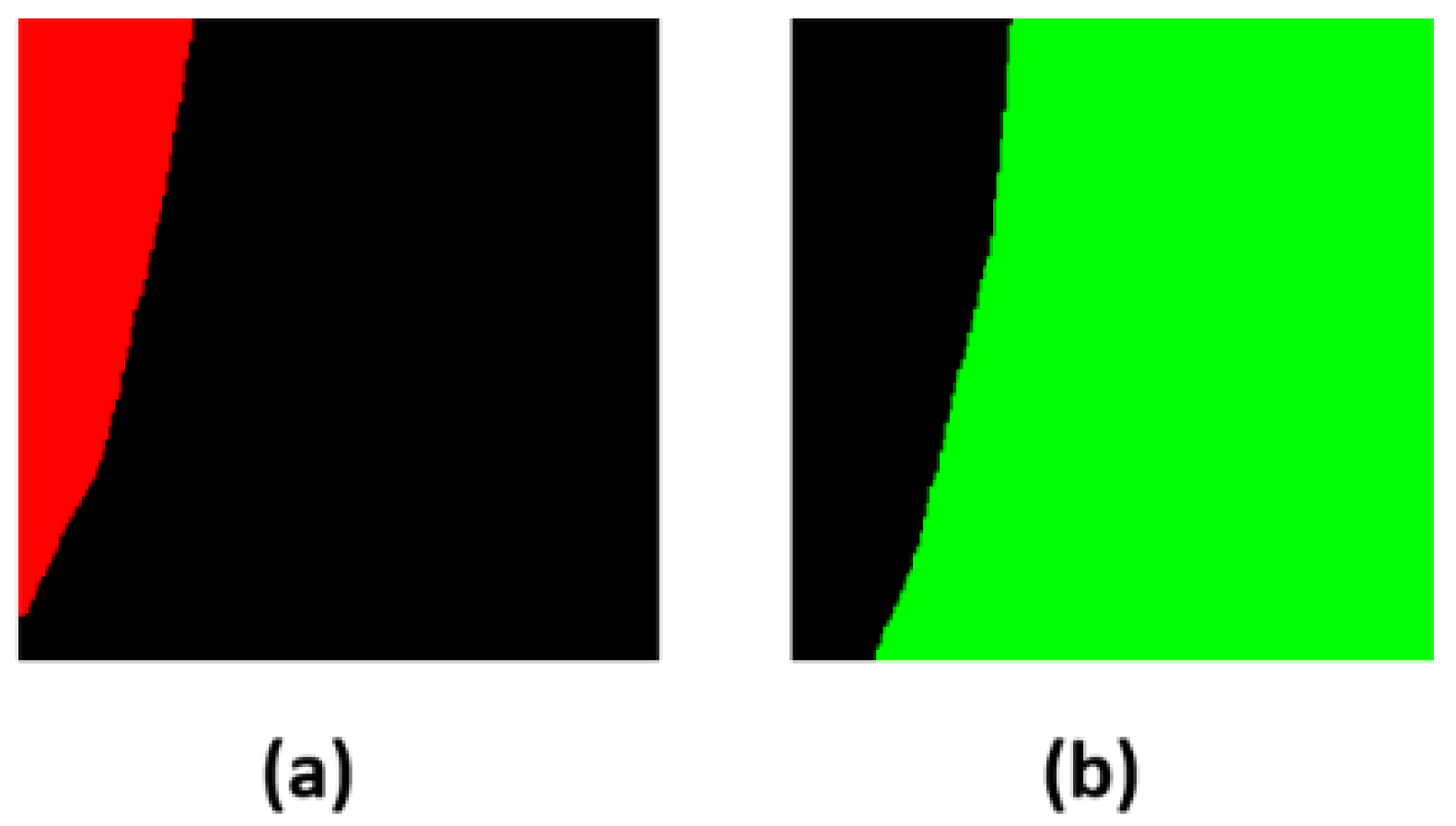
Figure 8.
Large-scale objects. It shows the large-scale objects of the image. We divided the image into two large-scale objects by the road. (a) is service_region, which contains small-scale object service_0; (b) is residence_region, which contains small-scale object service_1, green_space_0, and residence_0.
Figure 9.
The loss value of FCN during training. It shows the trend of loss values during training. From the figure, we can see that in the early period of the iteration (about before 5000 times), the loss value violently oscillated and then dropped sharply. In the medium term (around 5000–50,000), the loss value decreased slightly and tended to be stable. In order to ensure that the network has stabilized, we chose 60,000 as the number of iterations.
Figure 10.
Bleu_1 of different batch sizes. It shows the trend of Bleu_1 when the other parameters were constant and only the batch size was changed. As the batch size increased, Bleu_1 increased first and then decreased, and the effect of batch size on Bleu_1 was obvious, so a suitable batch size was necessary.
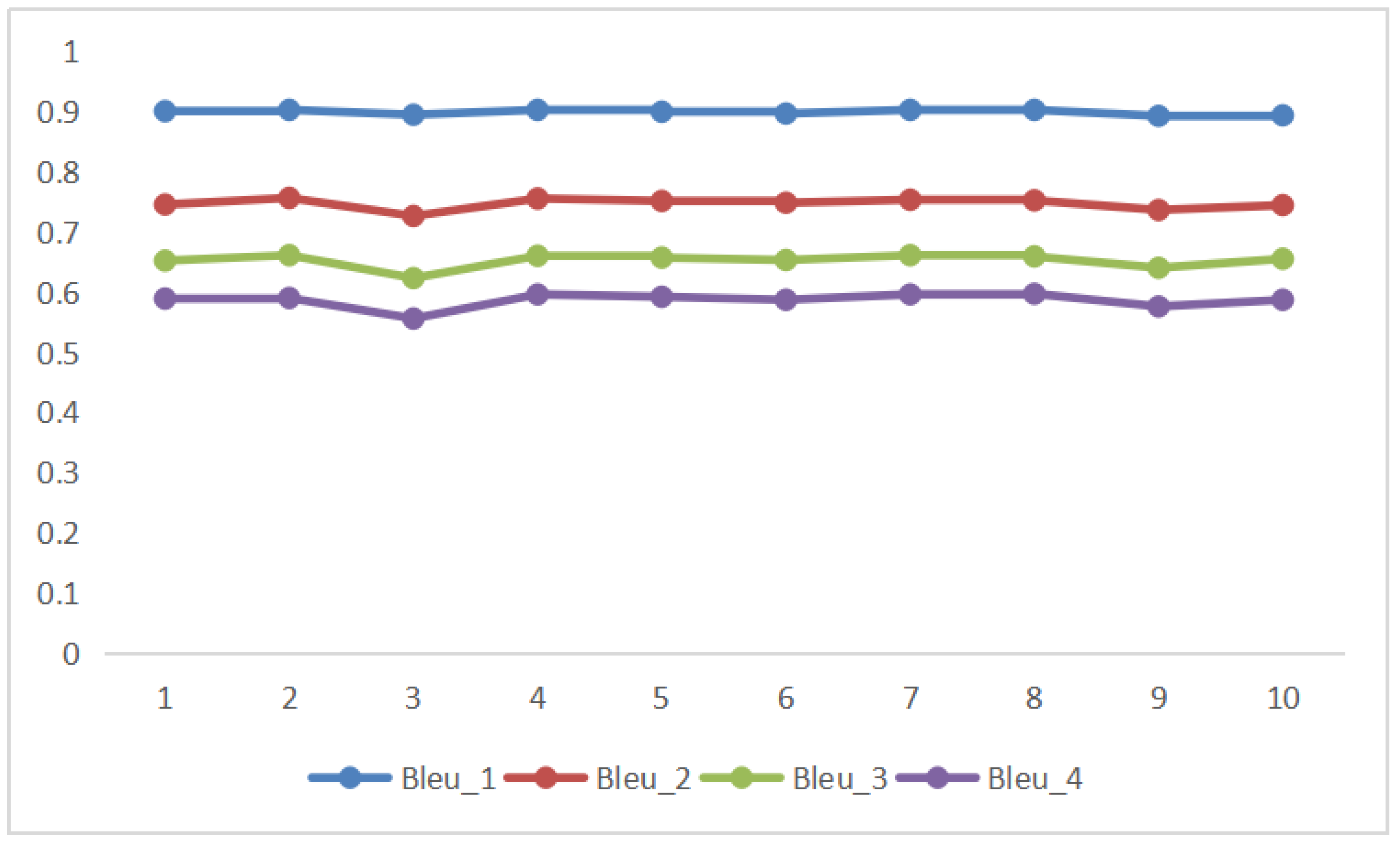
Figure 11.
Bleu trend of ten experiments. It shows the trend of Bleu. From the figure, we can see that in ten experiments, the variation amplitudes of Bleu_1, Bleu_2, Bleu_3, and Bleu_4 are small, which can prove the randomness of data distribution and the robustness of the algorithm.
Figure 11.
Bleu trend of ten experiments. It shows the trend of Bleu. From the figure, we can see that in ten experiments, the variation amplitudes of Bleu_1, Bleu_2, Bleu_3, and Bleu_4 are small, which can prove the randomness of data distribution and the robustness of the algorithm.
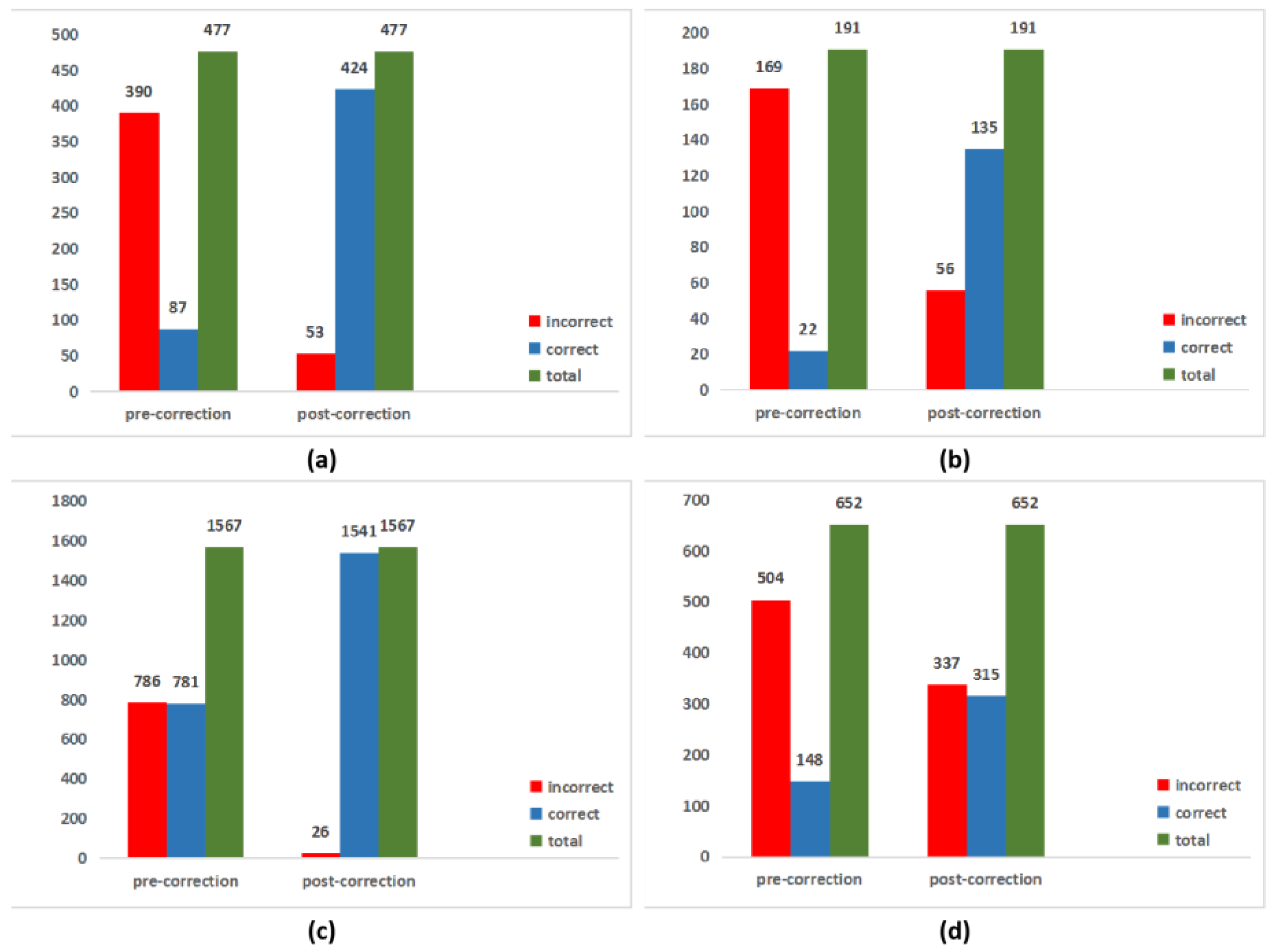
Figure 12.
Correction effect analysis. It shows the corrective effect of Sample Set 1 and Sample Set 2. (a,b) are the sample-based overall correction effect for Sample Set 1 and Sample Set 2, respectively; (c,d) are the noun-based overall correction effect for Sample Set 1 and Sample Set 2, respectively. As shown in the figure, whether from the perspective of samples or nouns, the correction algorithm proposed in this paper achieved good results. The correction effect of Sample Set 1 was better than that of Sample Set 2.
Table 1.
Classification of multiscale remote sensing objects.
Table 1.
Classification of multiscale remote sensing objects.
| Value | 10 | 11 | 12 | 13 | 14 |
| large-scale | residence region | industry region | service region | village region | forest region |
| value | 15 | 16 | 17 | 18 |
| large-scale | uncompleted region | road region | other region | Green-space region |
| value | 20 | 21 | 22 | 23 | 24 |
| small-scale | residence | industry | service | village | forest |
| value | 25 | 26 | 27 | 28 | 29 |
| small-scale | uncompleted | road | other | Green-space | waterbody |
Table 2.
Mean value of remote sensing objects.
Table 2.
Mean value of remote sensing objects.
| | The Mean Value of Weight at Every Object When Generating the First “Service” | The Mean Value of Weight at Every Object When Generating the Second “Service” |
|---|
| service_0 | 0.000061702 (correct) | 0.000016412 |
| service_1 | 0.000015618 | 0.000019851 |
| road_0 (with) | 0.000029001 | 0.000027496 |
| green_space _0 | 0.000015094 | 0.000023904 |
| residence_0 | 0.000021753 | 0.000046018 (incorrect) |
| service_region | 0.000061702 | 0.000016288 |
| residence_region | 0.0000164134 | 0.0000265598 |
Table 3.
Results comparison using VGG-19+LSTM.
Table 3.
Results comparison using VGG-19+LSTM.
| | Bleu_1 | Bleu_2 | Bleu_3 | Bleu_4 | METEOR | ROUGE_L | CIDEr |
|---|
| Ours | 0.774 | 0.535 | 0.406 | 0.314 | 0.359 | 0.663 | 2.745 |
| RSICD | 0.583 | 0.423 | 0.331 | 0.270 | 0.261 | 0.519 | 2.033 |
Table 4.
Comparing evaluation metrics.
Table 4.
Comparing evaluation metrics.
| | Bleu_1 | Bleu_2 | Bleu_3 | Bleu_4 | METEOR | ROUGE_L | CIDEr |
|---|
| Mean | 0.670 | 0.509 | 0.399 | 0.310 | 0.235 | 0.560 | 0.978 |
| Ours | 0.893 | 0.744 | 0.655 | 0.587 | 0.455 | 0.779 | 5.044 |
Table 5.
Reliability analysis for generated captions.
Table 5.
Reliability analysis for generated captions.
| Samples | Total Number of Samples: 668 |
|---|
| | Correct | Incorrect | Total |
|---|
| Words | 3417 | 368 | 3785 |
| Proportion | 90.28% | 9.72% | 100% |
| S.R. Word | 1396 | 170 | 1566 |
| Proportion | 89.14% | 10.86% | 100% |
| Nouns | 2021 | 198 | 2219 |
| Proportion | 91.08% | 8.92% | 100% |
Table 6.
Number of matched nouns before and after correction.
Table 6.
Number of matched nouns before and after correction.
| Samples | Total Number of Samples: 668 |
|---|
| | Pre-Correction Matched | Post-Correction Matched | Unmatched | Total |
|---|
| Nouns | 929 | 1856 | 363 | 2219 |
| Proportion | 41.87% | 83.64% | 16.36% | 100% |
Table 7.
The results of the overall analysis of the subsets.
Table 7.
The results of the overall analysis of the subsets.
| Samples | Total Number of Samples: 668 |
|---|
| | All Nouns are Correct: 477 | Not All Nouns are Correct: 191 |
|---|
| | Correct | Incorrect | Total | Correct | Incorrect | Total |
|---|
| S.R. Word | 1013 | 76 | 1089 | 383 | 94 | 477 |
| Proportion | 93.02% | 6.98% | 100% | 80.29% | 19.71% | 100% |
| | Pre-Correction Matched | Post-Correction Matched | Unmatched | Total | Pre-Correction Matched | Post-Correction Matched | Unmatched | Total |
| Nouns | 781 | 1541 | 26 | 1567 | 148 | 315 | 337 | 652 |
| Proportion | 49.84% | 98.34% | 1.66% | 100% | 22.70% | 48.31% | 51.69% | 100% |
Table 8.
Sample-based analysis of Sample Set 1 before and after correction.
Table 8.
Sample-based analysis of Sample Set 1 before and after correction.
| Sample Class | Completely Corrected | Partial Correction | No Corrective Effect | No Need for Correction | Total |
|---|
| Number | 337 | 37 | 16 | 87 | 477 |
| Proportion | 70.65% | 7.76% | 3.35% | 18.24% | 100% |
Table 9.
Sample-based analysis of Sample Set 2 before and after correction.
Table 9.
Sample-based analysis of Sample Set 2 before and after correction.
| Sample Class | Completely Corrected | Partial Correction | No Corrective Effect | No Need for Correction | Total |
|---|
| Number | 113 | 0 | 56 | 22 | 191 |
| Proportion | 59.16% | 0.00% | 29.32% | 11.52% | 100% |


