Automatic Recognition of Common Structural Elements from Point Clouds for Automated Progress Monitoring and Dimensional Quality Control in Reinforced Concrete Construction

Abstract

This manuscript provides a robust framework for the extraction of common structural components, such as columns, from terrestrial laser scanning point clouds acquired at regular rectangular concrete construction projects. The proposed framework utilizes geometric primitive as well as relationship-based reasoning between objects to semantically label point clouds. The framework then compares the extracted objects to the planned building information model (BIM) to automatically identify the as-built schedule and dimensional discrepancies. A novel method was also developed to remove redundant points of a newly acquired scan to detect changes between consecutive scans independent of the planned BIM. Five sets of point cloud data were acquired from the same construction site at different time intervals to assess the effectiveness of the proposed framework. In all datasets, the framework successfully extracted 132 out of 133 columns and achieved an accuracy of 98.79% for removing redundant surfaces. The framework successfully determined the progress of concrete work at each epoch in both activity and project levels through earned value analysis. It was also shown that the dimensions of 127 out of the 132 columns and all the slabs complied with those in the planned BIM.

1. Introduction

In construction projects, as-designed vs. as-built dimensional incompliances result in rework, which can cost up to 25% of the contracted construction cost [1]. In concrete structures, rework has shown to be a dominant factor in increasing concrete waste with the highest impact on project cost over-run due to waste, compared to other construction materials [2]. Concrete is in fact the most widely used material in the construction industry, used almost twice as much as other construction materials in the United States of America [3]. Not only does rework contribute to a direct cost over-run due to concrete waste, but it also causes an implicit cost to the environment since cement manufacturing accounts for about 5–7% of the global CO₂ emissions annually [4]. Other than the cost, time, and possible environmental impact associated with rework in concrete construction, dimensional errors and structural damages may impact structural integrity, diminishing safety during and after construction. One prime example of structural failure during construction is the 2018 pedestrian bridge collapse in Florida [5], which resulted in several fatalities. Early and accurate identification and reporting of delays, cost over-runs, rework, and structural instabilities through continuous inspection and as-built documentation are imperative to enabling project proponents to take corrective measures on time. An accurate and reliable as-built 3D/4D building information model (BIM) is not only beneficial during construction, but also during facility operations for maintenance work [6] as well as sustainability and waste management [7].

As-built documentation using traditional surveying methods, such as total station and measuring tape, is, however, labor-intensive, costly, and error-prone, particularly when performed frequently. In addition, only a portion of the site elements can be monitored for practicality as traditional instruments can only provide spot measurements [8]. To this end, the application of terrestrial laser scanners (TLS) for 4D as-built BIM documentation during construction is growing markedly, especially with the recent advancements in the speed and quality of data capture as well as the reduction in instrument cost. TLS acquires panoramic 3D coordinates of the surrounding surfaces, referred to as point clouds. TLS point clouds overcome the shortcoming associated with traditional single-point measurement instruments. However, due to the large amount of data, manual extraction of different structural components to generate a semantically rich BIM from the acquired point clouds is impractical, subjective, and error-prone [8]. Therefore, reliable and automated processing and semantic object extraction from TLS point clouds is essential to enabling its utilization in the construction industry for frequent and reliable as-built BIM documentation. To this end, this paper provides a new robust context-based framework for the extraction of primary structural components, namely column, slab, and rebar, in regular rectangular reinforced concrete structures from unorganized point cloud data for automated progress monitoring and dimensional conformity control during construction.

2. State of the Art in Semantic Extraction of Structural Components from Point Clouds

Comprehensive reviews of the recent developments in processing of point clouds acquired from construction sites and indoor environments can be found in [8,9,10,11,12,13,14]. Since the focus of this manuscript is the automated semantic extraction of structural components in regular rectangular concrete construction, the review of previous work is restricted to that addressing the specific problem of automated semantic labeling of objects with predominantly planar and linear facades. The presentation of the previous work in semantic feature extraction from point clouds is divided into the following three research categories:

• Scan vs. BIM, which is used only when a reliable as-planned 4D BIM exists;
• Supervised learning, which is used when an object template or library of preclassified similar objects exist for training/matching;
• Spatial and contextual relationship, which uses unique a prior knowledge of an object and its relationship to other objects.

2.1. Scan vs. BIM

Scan vs. BIM, initially proposed by Bosché [15,16,17], utilizes the as-planned 4D BIM to assign points to a BIM element in close spatial proximity. First, synthetic as-planned point clouds are generated by decomposing the planned BIM into points with the same spatial resolution of the point cloud. The as-planned and as-built point clouds are then registered through an iterative closest point (ICP) method, and corresponding points are matched by satisfying some spatial similarity criteria [8]. Once matched, the as-built point cloud is labeled as the element representing the as-planned point cloud. The scan vs. BIM method has been widely implemented in the previous literature for applications such as progress monitoring and reporting [18,19], extraction of formwork/rebars [20], and completion of rectangular concrete columns [21]. Scan vs. BIM is easy to implement and enables semantic labeling of key objects directly from BIM when a detailed planned BIM is available. The approach is, however, unreliable when the distance between the as-built and as-planned locations of an object is larger than the predefined spatial similarity criteria. In other words, the method works well when the planned and actual location of objects comply, which cannot be a presupposition since the objective of automated monitoring and control is to determine the discrepancies between the planned and actual location of each object [22]. Therefore, the studies presented in the following subsections aimed to reduce the dependency of the semantic object extraction on the details of the planned BIM.

2.2. Supervised Learning

An alternative to the scan vs. BIM method is to use a library of preclassified object attributes/features as templates for semantic feature extraction. For instance, a library of preclassified images were used as training data for a supervised learning sequence to find walls and construction materials in images taken from construction sites [23,24]. In point cloud processing, the preclassified object attributes can be generated through different means, such as the planned or as-built BIM [25,26], Monte Carlo simulation to generate synthetic point clouds of objects subject to random instrumental measurement errors [22], or manual classification of structural elements and its attributes from previously acquired point clouds [27]. To initiate the process, local curvature estimation together with planar/linear segmentation of raw point clouds are typically carried out. The features of each segment are then matched to the features of preclassified objects in the training datasets through a machine learning sequence for semantic labeling of the segment.

Reference [26] used features of preclassified point clouds of industrial components to label segmented points in the dataset that follow similar patterns. In [28], Rabbani’s region growing method [29] was adopted to segment planar surfaces of existing indoor buildings. The stacked supervised learning method [30] was then applied to classify the planar segments into objects such as walls, floors, and openings. Reference [31] first employed a combination of random sample consensus (RANSAC; [32]) and density-based attribute clustering (DBSCAN), as proposed by [33], to group together planar points of a completed indoor building. Eighteen geometric features, including the distance between a plane’s centroid and scan boundaries, were then calculated for each planar patch and fed to a k-means clustering and supervised learning framework to predict the object class (e.g., wall) that best matched the features. Their framework was able to correctly determine the object class of 71.2% of the segmented planes. Reference [27] aimed to extract concrete structures such as slabs, beams, and columns from point cloud data. First, points on concrete structures were isolated from other site objects using their color information through the method described in [34]. The remaining concrete points were then segmented through an edge-based segmentation procedure. For each segment, the level of linearity and planarity, as well as the directional axis, were estimated and assigned to a predefined class of objects (e.g., column) that best matched the estimated attributes through a support vector machine (SVM) classifier. For instance, a column is more linear than floors or walls and its directional vector is vertical. To populate the training data, a large library of historic point cloud datasets of each object class was used to manually estimated the suggested features (i.e., level of planarity/linearity).

The application of machine learning for semantic labeling of point clouds is suitable for the extraction of complex geometries or repeatable objects, such as in the case of the manufacturing industry. However, it requires a library of preclassified object attributes or historical point clouds from similar objects to populate the training data, which may neither be readily available nor always practical. To this end, the research studies presented in the following subsection only used spatial and contextual relationships between objects (also referred to as hard-coded knowledge in [14]) for semantic labeling.

2.3. Spatial, Geometrical, and Contextual Relationship

An alternative to the aforementioned methods uses only the logical and unique spatial and geometrical relationships between different object types to semantically label planar segments [9,35]. For instance, a segmented planar surface of an indoor room can be a wall, floor, ceiling, or clutter. However, due to the generic arrangement of rooms, the following relationships can be inferred:

• Floors and ceilings are predominantly in horizontal planes [22];
• Walls are in vertical planes orthogonal to the floors/ceilings [36];
• Walls span from the floor to the ceiling [37];
• Segment sizes of permanent components (walls, floors) are likely larger than clutter [38]; and so on.

Using contextual information of the specific object of interest, it is possible to semantically label surfaces in the point cloud that follow similar characteristics. This process typically starts with some method of local curvature estimation, followed by planar/linear segmentation (region growing or clustering). The contextual hard-coded knowledge for each class of object (e.g., column and walls) is then used to semantically label each planar (or linear) patch that satisfies the object’s conditions.

Reference [38] used prior information of common building objects (e.g., façade and window) to semantically label planar segments collected from the exterior of existing buildings. The framework first applies the segmentation method of [39] to extract planar segments. The planar segments are then assigned to a predefined class of objects (e.g., wall, ground, window, etc.) using some prior information about their relative size, position, orientation, topology, and point density. These categories of a priori relationships were also employed in [40] for semantic labeling of the exterior of existing buildings.

The RANSAC method, proposed in [32], was employed in [36,41,42] with thresholds tuned to the specific dataset to extract planar surfaces of existing indoor rooms before semantic object extraction. In [36], planar segments whose normal vector was parallel and perpendicular to the x−y plane were then considered as floor/ceilings and walls, respectively. In [42], slabs and walls were detected when two proximate planar surfaces with parallel normal vector in opposing directions were found. Reference [37] proposed a semiautomated method for the generation of BIM models of existing indoor buildings. First, points from different floor levels were extracted using the histogram of floor height (for example, in [22,43]). Points within each floor were then projected onto the x−y plane to create a binary (grayscale) image to determine the boundaries of each room. For each room, walls were differentiated from occlusions based on the points’ proximity to both the ceiling and floor. Proximate parallel walls of two adjacent rooms were then labeled as one wall (similar to [42]). In [44], the histogram of point height was also used to determine points of the same floor level in existing indoor buildings through some predefined bin size and prior knowledge of the thickness of the slab. Reference [45] proposed a method to extract columns with rectangular and circular cross sections directly from the point cloud. Since the orientation of columns were assumed to be vertical, the point cloud was first projected onto the x−y plane and converted into a grayscale image (similar to [37]). A 2D Hough transform was then adopted to extract circular and rectangular objects from the binary image. The results showed that rectangular cross sections were prone to Type I errors, while circular cross sections were prone to Type II errors.

Many previous studies focused on the extraction of architectural and exterior components, such as walls and windows, from existing buildings (after completion of construction) [36,37,38,40,41,42,44]. However, point clouds acquired from construction sites contain outliers due to dust, occlusions, and moving objects, which requires additional robust outlier removal procedures [22]. Other group of studies that focus on semantic labeling of point clouds acquired from construction sites mainly require either an up-to-date 4D BIM [15,16,17,18,19,20,21,22,25] or a library of historical preclassified objects [23,24,26,27,28,31], which may be neither available nor practical. In addition, to provide a generalizable solution, a point cloud processing framework is required whose effectiveness is independent of subjectively predefined thresholds [22]. This study provides a robust solution to the semantic labeling of common reinforced concrete elements from point clouds using the spatial relationship, method of construction, and systematic thresholds, adopted from reliable standards of reinforced concrete construction.

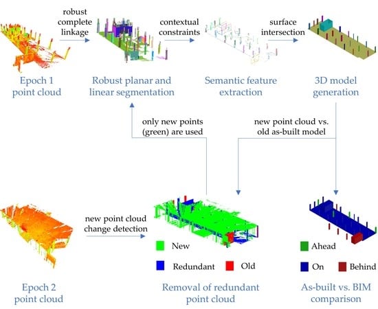
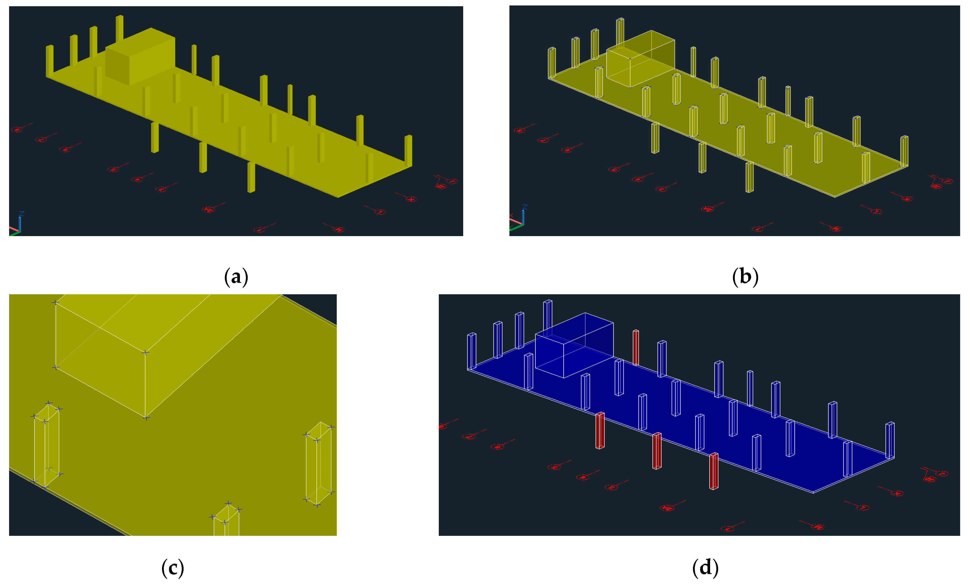
3. Methodology

This manuscript focuses on the robust extraction of common structural elements, columns, rebars, and slabs from point clouds acquired from regular rectangular reinforced concrete structures for progress monitoring and dimensional compliance control. Regular rectangular reinforced concrete structures are targeted here specifically, since they are commonly employed in the building construction industry [3,46,47]. The overview of the methodology is as follows:

• Robust extraction of planar and linear features from registered point clouds (Figure 1b);
• Semantic labeling of point clouds into floors, columns, and rebars using contextual and spatial information (Figure 1c);
• Surface intersection and modeling (Figure 1d);
• Identification and visualization of deviations between as-built and planned BIM (Figure 1g); and
• Removal of redundant points of previously modeled surfaces for newly acquired point clouds (Figure 1f). For prospective scans, the processes described in steps 1–4 will only be carried out for the new points (shown in green; Figure 1f).

3.1. Target-Based Point Cloud Registration

The convention proposed in [8,22] is used to register point clouds to a reference coordinate system (the coordinate system of the planned BIM). This approach uses signalized TLS targets on presurveyed site control points to register coordinate systems of scans at each epoch to a reference coordinate system. The centers of the signalized targets are measured through high-precision surveying and the TLS instrument. The centers of targets are matched to estimate the exterior orientation parameters along with registration precision through rigid body transformation.

3.2. Robust Planar and Linear Segmentation

As illustrated in Figure 1b, planar and linear segmentation is the first step towards semantic extraction of concrete elements. Here, the method developed in [22] is employed for robust planar and linear segmentation. The method is specifically adopted since it is robust to common outliers of construction site point clouds and the segmentation results are not a function of a subjectively predefined threshold. According to this method, horizontal planes are first extracted using the histogram of point height (similar to [37,43]) to promote computational efficiency. The horizontal plane extraction method used in [22] is robust to Type II errors and was shown to be effective in extracting floor objects from construction site environments. The remaining points are then classified into planes and lines using a robust principal component analysis (PCA) method to determine local surface curvature. The local surface curvature values are then matched to that obtained by Monte Carlo point cloud simulations, subjected to random measurement errors, to determine the final set of planar and linear points. The classified planar and linear features are then segmented into surfaces with similar geometrical attributes using a new iterative and robust variation of the complete linkage hierarchical clustering method.

3.3. Semantic Object Extraction Using Relationship-Based Reasoning

Here, the objective is to extract flat slab floors, rectangular columns, and rebars from the segmented planar and linear features. For floors, the method developed in [22] is used since it was consistently able to extract floors from other possible horizontal objects in various construction site settings. The problem is now reduced to the semantic extraction of rectangular columns and rebars from other elements. Figure 2 shows the point cloud of a typical column before and after the slab of the top floor is poured. The exposed rebars on the top of the columns in Figure 2a enable the seamless transfer of stresses and bending moments between floors. After the concrete for the top floor slab is poured, these rebars are no longer visible (Figure 2b). From Figure 2, it can be observed that rebars are linear features on top of columns. Figure 2 also shows that rectangular columns are confined by a floor object at the bottom and either linear objects (rebars) or a floor object (ceiling) on the top.

Another important characteristic of structural columns is its responsibility to transfer the bending moments and vertical stresses from top floors to the foundation. For regular rectangular buildings, columns are almost always oriented in the direction of the two orthogonal main axes of the rectangular plan to accommodate consistent load transfer [3,47,48]. The consistent column orientation is also desirable to preserve symmetry. Therefore, by examining the orientation as well as the objects surrounding the boundaries of planar surfaces, planar surfaces representing columns can be uniquely identified. These two criteria are used to distinguish columns from other planar objects on sites. Once the columns are identified, rebars objects are linear segments on top of the columns. The solution to the column extraction is formulated as follows:

• Algorithm 1: First, the two main orthogonal orientation directions of planar surfaces, excluding the floor objects, are identified. The planar surfaces whose normal vectors are in the same direction of these two vectors are selected as potential column candidates (i.e., planes whose normal vector follows the direction of the main orthogonal site axes).
• Algorithm 2: The boundaries of the extracted planar candidates are then assessed to determine the presence of floor and/or linear objects in the proximity of their exterior boundaries.

3.3.1. Algorithm 1: Detection of Planes Following the Main Orthogonal Site Axis

• Select the planar surfaces, excluding the floor objects.
• Assign the normal vector associated with the planar surface to each point of that segment.
• Estimate the mode of the bivariate x−y components of the normal vectors. In this study, the mean-shift mode detection [49] with a normal kernel and optimized fixed-bandwidth proposed by [50] was adopted.
• For every two identified modes, calculate the allowable standard deviation of the inner product of two modes, ${\sigma }_{⟨\stackrel{\rightharpoonup }{n_i},\stackrel{\rightharpoonup }{n_j}\rangle }$, derived by applying the law of variance propagation, using Equation (1):

  $${\sigma }_{⟨\stackrel{\rightharpoonup }{n_i},\stackrel{\rightharpoonup }{n_j}\rangle }^2=2{\sigma }_{\theta }^2\left(1-\left({\cos }^2{\theta }_{x_i}{\cos }^2{\theta }_{x_j}+{\cos }^2{\theta }_{y_i}{\cos }^2{\theta }_{y_j}+{\cos }^2{\theta }_{z_i}{\cos }^2{\theta }_{z_j}\right)\right),$$

  (1)

  where $\stackrel{\rightharpoonup }{n_i}$ and $\stackrel{\rightharpoonup }{n_j}$ are the normal vectors of the i^th and j^th mode, respectively; ${\sigma }_{⟨\stackrel{\rightharpoonup }{n_i},\stackrel{\rightharpoonup }{n_j}\rangle }$ is the allowable tolerance of the inner product of vectors $\stackrel{\rightharpoonup }{n_i}$ and $\stackrel{\rightharpoonup }{n_j}$; ${\sigma }_{\theta }$ is the allowable angular tolerance in radians; $⟨{\theta }_{x_i},{\theta }_{y_i},{\theta }_{z_i}\rangle$ are the angles of the normal vector of the i^th mode to the x, y and z axes, respectively; and $⟨\stackrel{\rightharpoonup }{n_i},\stackrel{\rightharpoonup }{n_j}\rangle$ is the inner product of vectors $\stackrel{\rightharpoonup }{n_i}$ and $\stackrel{\rightharpoonup }{n_j}$. In this study, the allowable plumb tolerance (${\sigma }_{\theta }$) is set to approximately 0.52°, derived from ACI 117 [51,52].
• Select the two modes whose absolute value of the inner product satisfies the orthogonality criteria of Equation (2):

  $$\left|⟨\stackrel{\rightharpoonup }{n_i},\stackrel{\rightharpoonup }{n_j}\rangle \right|\le 3{\sigma }_{⟨\stackrel{\rightharpoonup }{n_i},\stackrel{\rightharpoonup }{n_j}\rangle },$$

  (2)
  The threshold $3{\sigma }_{⟨\stackrel{\rightharpoonup }{n_1},\stackrel{\rightharpoonup }{n_2}\rangle }$ is used to account for approximately 99% confidence.
• For the pair of normal vectors satisfying Equation (2), find the normal vectors of the planar surfaces whose angles are within $\pm 3{\sigma }_{\theta }$ in each direction.

The surfaces satisfying step 6 are the surfaces whose normal follows the direction of the main site axes. Other than identifying surfaces following the main site axes, the algorithm can also identify surfaces that are not built to the specified tolerances in relation to the majority of the built surfaces before a plan vs. actual comparison is even performed. The two main orthogonal axes can also be used to improve registration of point clouds in the absence of reliable target-based registration.

3.3.2. Algorithm 2: Assessment of Column Boundary Conditions

• Select the planar candidates obtained from Algorithm 1.
• Calculate the first and third quartile of the height of all planar candidates.
• Identify planar surfaces whose minimum height is smaller than the first quartile, and maximum height is larger than the third quartile of height (to ensure removal of shorter clutters).
• Identify the outer boundary points of each planar segments using α-shapes [53,54], following the method described in [22].
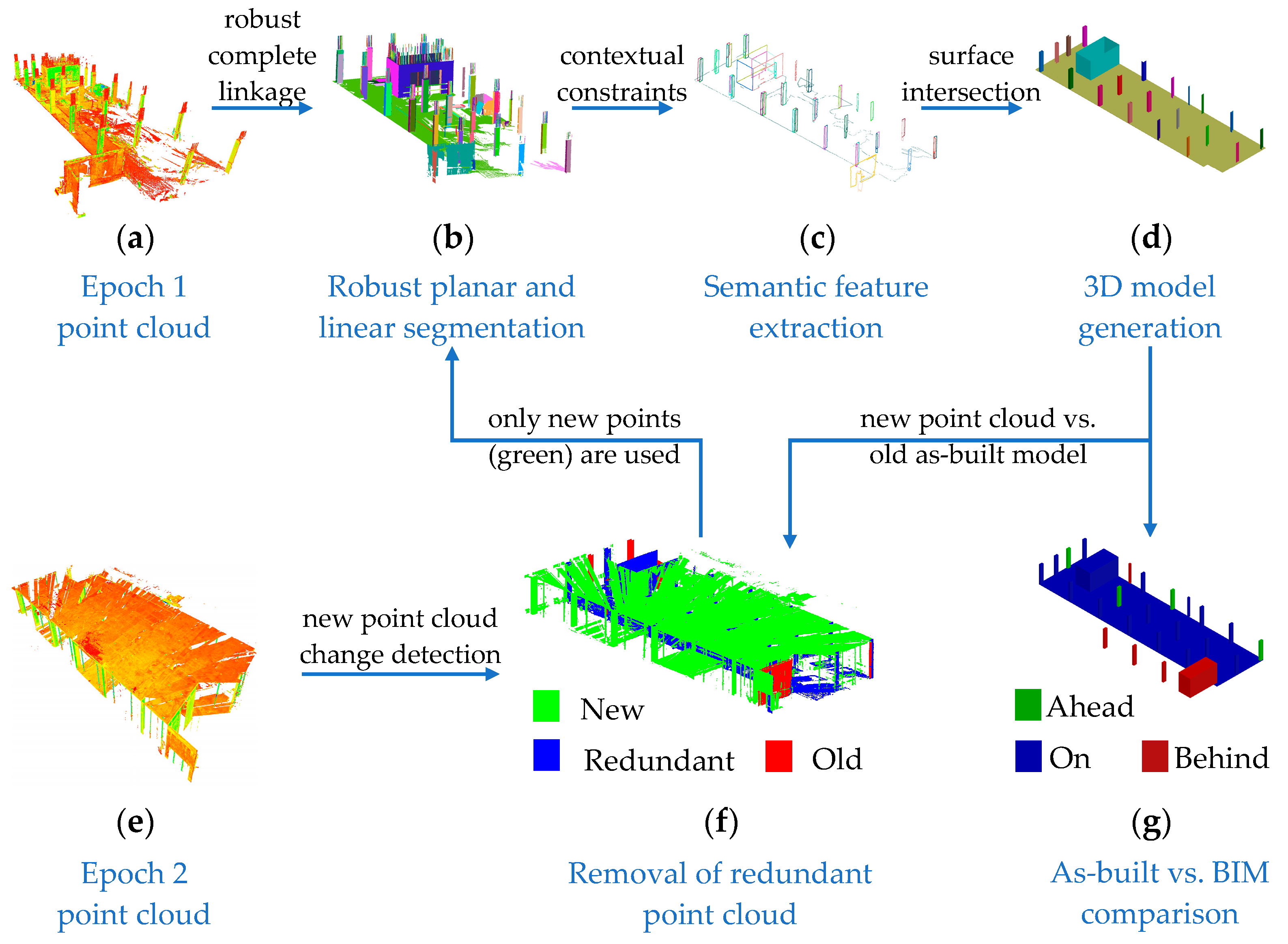
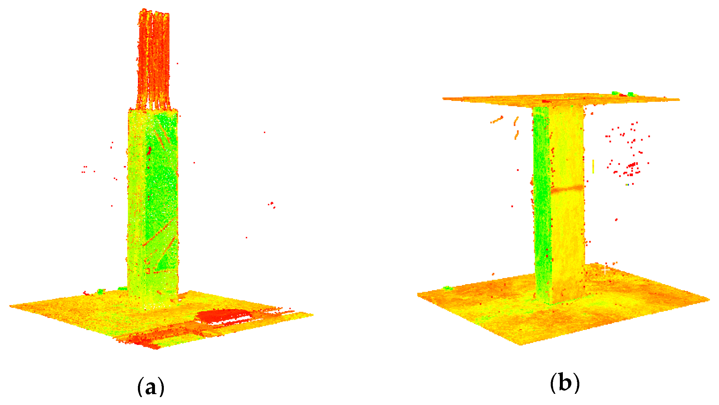
• Perform connected components region growing (Algorithm 5 of [8]) on the identified boundaries to group together potential columns. Here, the neighborhood size is set to $r\sqrt{2}$, where $r$ is the radius of the neighborhood used for robust PCA classification [22]. This neighborhood size was chosen since the local neighborhood of points within $r$ from the edge of two intersecting surfaces are prone to misclassification using classical PCA (see Figure 3b,c). Since robust PCA classifies more planar points closer to the boundaries than classical PCA [22,43], the defined threshold will be large enough to group together surfaces of the same column.
• Select the connected segments that contain a floor object within $r$ from its minimum height ($r$ is used for the same reasons given in step 5 and Figure 3c).
• From the remaining connected segments satisfying step 6, a connected segment is labeled a column if one of the following two criteria is satisfied:
  • The largest height of the segment is within $r$ from the median height of a floor object; or
  • A linear segment within $\sqrt{{\left(2r\right)}^2+{\left(rebar cover size\right)}^2}$ (derived from the Pythagorean theorem) of the boundaries of the connected segment exists. The cover size, schematically shown in Figure 3d, is set to 50 mm following ACI 318 (2014) [55].

Once the columns are extracted using Algorithms 1 and 2, the enclosed linear segments are labeled as rebar objects using Algorithm 3: Semantic Rebar Extraction, as follows:

• Select the column segments from Algorithm 2 that satisfy the condition of step 7b.
• For each column segment, identify all linear segments whose minimum height is larger than the column’s height.
• Project all identified linear segments onto the x−y plane.
• The linear segments whose boundaries in the x−y plane are enclosed by the boundaries of the columns are considered as rebars.

3.4. Parametric Surface Representation

After the floors, rebars, and columns have been automatically extracted from the segmented point cloud, it is important to provide a parametric model to represent the as-built for comparison with the planned BIM. The parametric representations of the identified objects are as follows:

• Floors: every floor is represented by a normal vector (estimated through robust PCA), and a point on the plane (robust center of the points) [22]. The boundary of the floors is identified using the modified convex hull algorithm and boundary regularization presented in [56] to define the extents of the floor planes.
• Rebars: each rebar is represented by a point (e.g., robust center of the segmented rebar), length of the rebar, cylinder’s axis, and radius. The radius and cylinder’s axis are estimated through Algorithms 1 through 3 of [8] to provide an accurate and robust estimation. To define the length of the cylinder, rotate the cylinder’s axis to the z direction using Rodrigues rotational formulation. The length of the rebar is then the difference between the maximum and minimum heights of the rotated rebar.
• Columns: the extents of the rectangular columns are defined by the eight vertices of the rectangular prism (Figure 2b). Each planar façade of the column is represented by the four plane parameters (see floor objects above). The bottom vertices are estimated through the intersection of planar surfaces and the floor object on the bottom. The process is identical in cases where a floor object also exists on the top (i.e., ceiling; see Figure 2b). In cases where only rebars exist on top, a virtual plane parallel to the bottom floor plane with distance of the maximum height of the column segment from the bottom floor is generated. The top four vertices are calculated accordingly through planar intersection.

3.5. Planned vs. As-Built Comparison

As explained in Section 3.1, the scans are registered to the reference coordinate system of the planned BIM following the convention proposed in [8,22]. To compare the planned and the as-built, the corresponding objects between the plan and as-built are identified using a distance threshold. Following the convention set forth by [15,16,17,18], a 50 mm distance threshold is suggested as expected construction errors. Figure 4a represents the planned 4D model of a construction site at a given baseline. Figure 4b,c show the superimposition of the planned model and the automatically identified columns at the baseline. The blue crosses in Figure 4c represent the generated edges (8 vertices) of the identified columns using the method presented in Section 3.4. The objects whose minimum distance is smaller than 50 mm are then identified. The progress can then be visually presented through a color-coding scheme. In Figure 4d, blue represents on-schedule activities (identified objects), the red color represents behind-schedule activities (not found), and green objects (not shown in the presented example) are ahead of schedule activities.

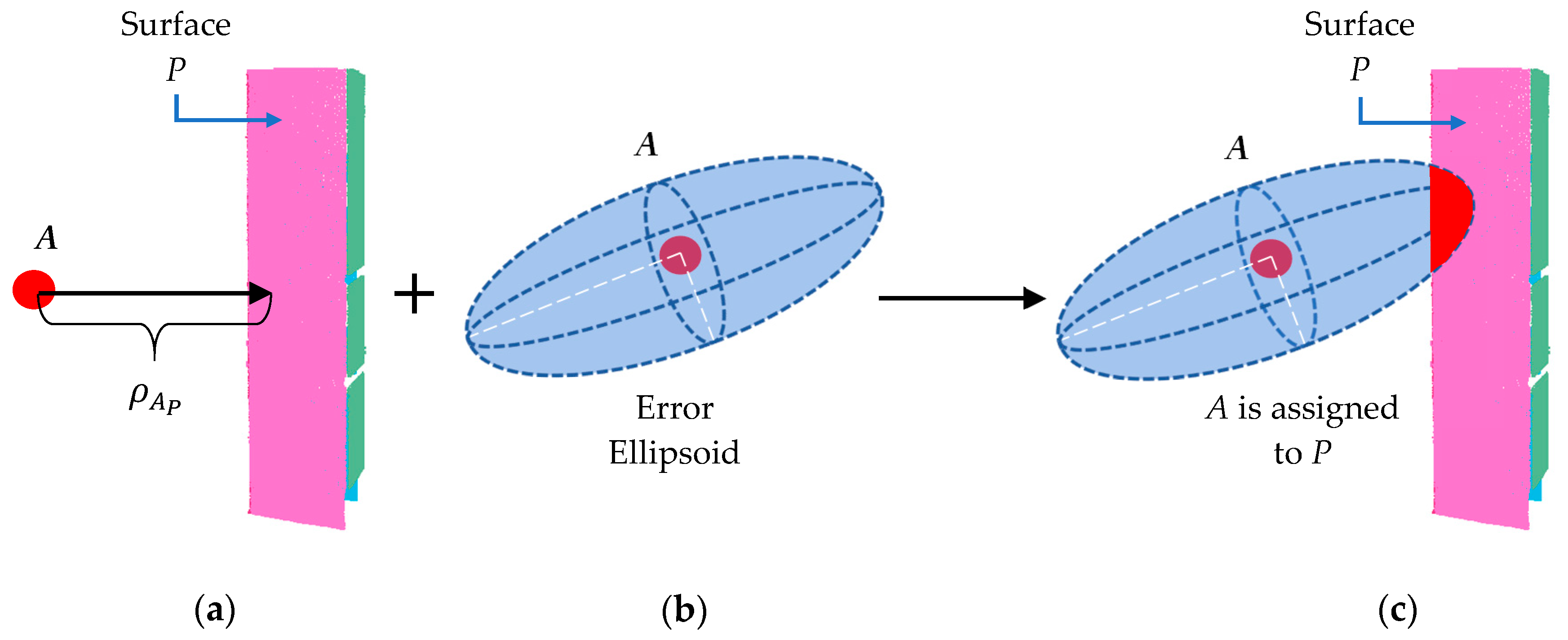
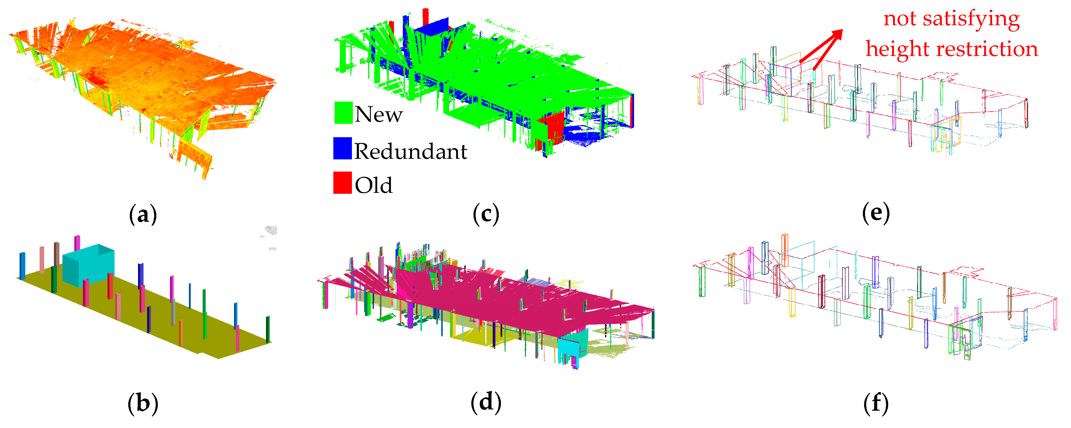
3.6. Redundant Point Removal of Prospective Scans

Since the process of monitoring and control is carried out in a continuous manner, it is possible that a newly acquired scan contains points of objects that were modeled from previous scans. It is, hence, desirable to remove these points first before point cloud processing so that only the new changes in structural components are detected.

Consider a newly acquired scan $j$ registered to the reference coordinate system (object space), following the convention proposed in Section 3.1. The objective is to identify if point A (Figure 5a) of scan $j$ is close enough to a presegmented object surface P to be considered as a point on surface P. To this end, an error ellipsoid (Figure 5b) is estimated around point A that accounts for both scanner observational as well as registration uncertainties. Point A of scan $j$ is considered redundant if a presegmented surface P in the object space exists such that the error ellipsoid has an intersection with surface P (Figure 5c). Point A is then semantically labeled as the object represented by surface P.

To determine the error ellipsoid, the covariance of the radiated point $i$ from scanner space $j$ to the object space (reference coordinate system) is calculated through the law of variance propagation as follows:

$${\left[\begin{array}{c}x\\ y\\ z\end{array}\right]}_{ij}=r_{ij}=M_j\left({\left[\begin{array}{c}X\\ Y\\ Z\end{array}\right]}_i-{\left[\begin{array}{c}X\\ Y\\ Z\end{array}\right]}_j^c\right)=M_j\left(R_i-R_j^c\right)\to R_i=M_j^T{r}_{ij}+R_j^c,$$

(3)

$$C_{r_{ij}}=\left[\begin{array}{ccc}{\sigma }_{\rho }^2{\sec }^2{\beta }_{ij}& 0& 0\\ 0& {\sigma }_{\theta }^2& 0\\ 0& 0& {\sigma }_{\alpha }^2\end{array}\right],$$

(4)

$$C_{R_i}=\frac{\partial R_i}{\partial x_e}{C}_{x_j}{\frac{\partial R_i}{\partial x_e}}^T+\frac{\partial R_i}{\partial r_{ij}}{C}_{r_{ij}}{\frac{\partial R_i}{\partial r_{ij}}}^T,$$

(5)

where $r_{ij}$ is the observed scanner space vector of point $i$ in space $j$, $R_i$ is the object space vector of point $i$, $R_j^c$ is the object space vector of scanner $j$ (translation vector), $M_j$ is the rotation matrix from object space to scanner space $j$, $C_{r_{ij}}$ is the covariance matrix of observation $i$ in scanner space $j$, ${\sigma }_{\rho }^2$ is the instrumental range error variance at normal incidence, ${\sigma }_{\theta }^2$ and ${\sigma }_{\alpha }^2$ are the instrumental angular variances, ${\beta }_{ij}$ is the incidence angle of observation $i$ collected from scan $j$, $x_e$ is the set of registration parameters, and $C_{x_j}$ is the covariance matrix of registration parameters for scan $j$. Using the covariance matrix of Equation (5), an error ellipsoid is constructed with 95% confidence and three degrees of freedom (three-dimensional data). Using the derived equations, the redundant surfaces are removed following Algorithm 4: Redundant Surface Extraction:

• For every new scan point, $i$, calculate the covariance matrix, $C_{R_i}$ using Equation (5).
• Calculate the eigenvalues ($\lambda )$ and eigenvectors ($v$) of the covariance matrix ($C_{R_i}$).
• Construct error ellipsoid using Equation (6):

  $${\left(X-R_i\right)}^{T}v{\lambda }^{-1}{v}^T\left(X-R_i\right)={\left(X-R_i\right)}^{T}v{\left({\lambda }^{-\frac{1}{2}}\right)}^T{\lambda }^{-\frac{1}{2}}{v}^T\left(X-R_i\right)\le {\mathcal{X}}^2{}_{0.95,3}$$

  (6)

  where $R_i$ is the vector of coordinates of point $i$ in the object space and ${\mathcal{X}}^2{}_{0.95,3}$ is a chi-squared probability with 95% confidence and 3 degrees of freedom (${\mathcal{X}}^2{}_{0.95,3}=7.8147$).
• Find all planar and cylindrical (rebars are modeled as cylinders; see Section 3.4) objects from Algorithms 1–3 that intersect the error ellipsoid.
• If more than one surface meets the conditions of step 4, the point is assigned to the closest surface. The point is then semantically labeled to the corresponding object represented by the segmented surface.

Step 4 of Algorithm 4 requires a procedure to find the intersection between an ellipsoid and a plane as well as a cylinder, which is not trivial. Here, two original and generic algorithms (Algorithms 5 and 6) are developed to identify the intersection of a plane/cylinder and ellipsoid in space.

3.6.1. Algorithm 5: Intersection of an Ellipsoid and Plane

• Calculate the distance of the point to the planar segments (${\rho }_{A_P}$ of Figure 5a).
• Identify all surfaces where ${\rho }_{A_P}$ is smaller than $\sqrt{{\lambda }_{max}{\mathcal{X}}^2{}_{0.95,3}}$, the semimajor axis.
• Calculate the linear transformation matrix ${\lambda }^{-\frac{1}{2}}{v}^T$ that transforms the error ellipsoid of Equation (6) into a sphere with radius $\sqrt{{\mathcal{X}}^2{}_{0.95,3}}$. This transformation reduces the problem to finding the intersection between a sphere and a plane, since planes are affine equivariant.
• Calculate the distance of point $i$ from each transformed planar segment ($p_d$).
• Identify all surfaces whose distances ($p_d$) are smaller than $\sqrt{{\mathcal{X}}^2{}_{0.95,3}}$.
• Project the transformed error sphere onto the surfaces satisfying condition 5 to construct an error circle with the point’s projection as the center and radius $\sqrt{{\mathcal{X}}^2{}_{0.95,3}-p_d^2}$ (Pythagorean theorem).
• The point is assigned to the surface if and only if its projected circle intersects with the boundary of that surface.

3.6.2. Algorithm 6: Intersection of an Ellipsoid and Cylinder

• Calculate the distance of the point to the axis of the cylindrical segments $\left({\rho }_{A_L}\right)$.
• Identify all cylinders where ${\rho }_{A_P}$ is smaller than $\sqrt{{\lambda }_{max}{\mathcal{X}}^2{}_{0.95,3}}+r_{cyl}$, where $r_{cyl}$ is the radius of the cylindrical segment.
• Find the rotation matrix, $M_{cyl}$, that orients the cylinder’s axis parallel to the z-axis following Rodrigues rotation formula.
• Rotate the error ellipsoid (Equation 6) and the cylindrical segment using $M_{cyl}$.
• Project the rotated ellipsoid and cylinder onto the x−y plane. This reduced the problem to finding the intersection between a circle and an ellipse in a 2D plane. To this end, we first identify the closest point, $P_{Closest}$, from the center of the circle ($O_{cyl}$) to the ellipse using the following steps.
• Calculate the transformation matrix ${\lambda }^{-\frac{1}{2}}{v}^T{M}_{cyl}^T$ of the newly rotated error ellipse.
• Transform the error ellipse into an error circle with radius $\sqrt{{\mathcal{X}}^2{}_{0.95,3}}$ and center, $O_{elp}$.
• Transform the center of the circle, $O_{cyl}$, into $O_{Trans}$ using the same transformation matrix as step 6. This transformation further reduces the problem to identifying the closest point between the newly transformed point ($O_{Trans}$) and error circle of step 7.
• Calculate the point of intersection, $P_{Trans}$, between the line segment $O_{Trans}-O_{elp}$ and the error circle.
• Identify $P_{Closest}$ by transforming the point of intersection, $P_{Trans}$, back to the correct coordinate system (i.e., before the affine transformation of step 6).
• Identify all segments where the distance between $P_{Closest}$ and $O_{cyl}$ is smaller than the radius, $r_{cyl}$ (the condition for the intersection of the ellipse and circle).
• Project the rotated error ellipsoid of step 4 onto the $z$ axis. Identify the maximum and minimum height of the projected ellipsoid. The point is assigned to the surface if and only if its projected height intersects with the height of the cylindrical segment.

3.7. Method of Validation of Results

To assess the effectiveness of the object classification as well as the redundant surface extraction, the precision, recall, and accuracy are estimated following the definitions presented in [57]:

$$Precision=\frac{{\mathrm{T}}_P}{{\mathrm{T}}_P+F_P},$$

(7)

$$Recall=\frac{{\mathrm{T}}_P}{{\mathrm{T}}_P+F_n},$$

(8)

$$Accuracy=\frac{{\mathrm{T}}_P+{\mathrm{T}}_N}{{\mathrm{T}}_P+{\mathrm{T}}_N+F_P+F_N}$$

(9)

where ${\mathrm{T}}_P$,${\mathrm{T}}_N$, $F_P$, and ${\mathrm{F}}_N$ are the number of true positive, true negative, false positive, and false negative counts, respectively. The ground truth is determined through manual extraction.

Planned vs. as-built comparison for progress monitoring and dimensional compliance is also performed. For progress reporting, the well-established earned value management (EVM) is used to determine the project’s performance at different epochs. For dimensional quality control, the dimensions of structural components such as columns were compared to the design as well as ground truth measurements. For each epoch, the percentage of columns passing the standard dimensional tolerances is also determined. The ground truth measurements for the required object dimensions were manually estimated using measuring tape. To calculate the horizontal (two-dimensional) accuracy, the distance root mean squared (DRMS) [58] is used. To calculate the one-dimensional accuracy, such as in the case of slab thickness, the absolute deviation is used.

4. Experimental Results

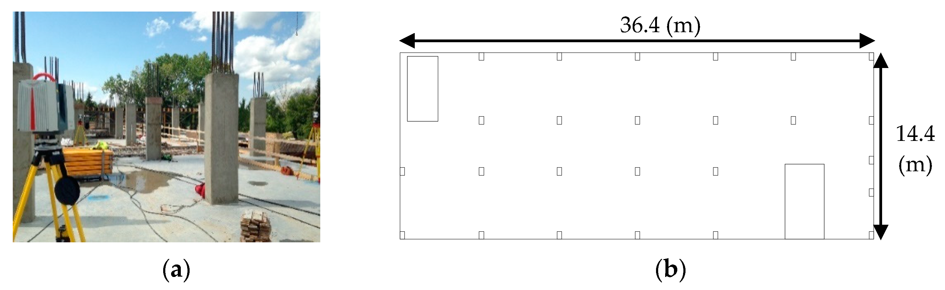
4.1. Experiment Description

Five sets of TLS point clouds were acquired from the Graduate Student Hall of Residence (GSHR) construction site (Figure 6) at the University of Calgary. The objective of this experiment was to automatically monitor the progress of concrete work on a specific portion of the site (Figure 6b). The building structure is comprised of cast-in-place reinforced concrete with flat slab floors, steel rebars, and rectangular columns. The planned schedule for the completion of the concrete work for each floor was one week; hence, the site was monitored roughly once every week for a duration of five weeks. For each floor, one dataset was collected after the scheduled completion of the columns of the floor, and another just after the completion of the slab of the floor above. The point cloud data was acquired using the Leica HDS6100 TLS [59]. The scans were registered to the planned model reference coordinate system using signalized targets on presurveyed site control points as described in Section 3.1. The number of points, number of scan stations, and registration precision per epoch is provided in

Table 1. Number of scan stations, number of points, and registration precision per epoch.

Epoch	No. of Scan Stations	Total No. of Points (millions)	Registration Precision (mm)
1	3	37	1.5
2	3	153	1.4
3	4	201	2.2
4	3	115	1.5
5	5	358	1.8

.

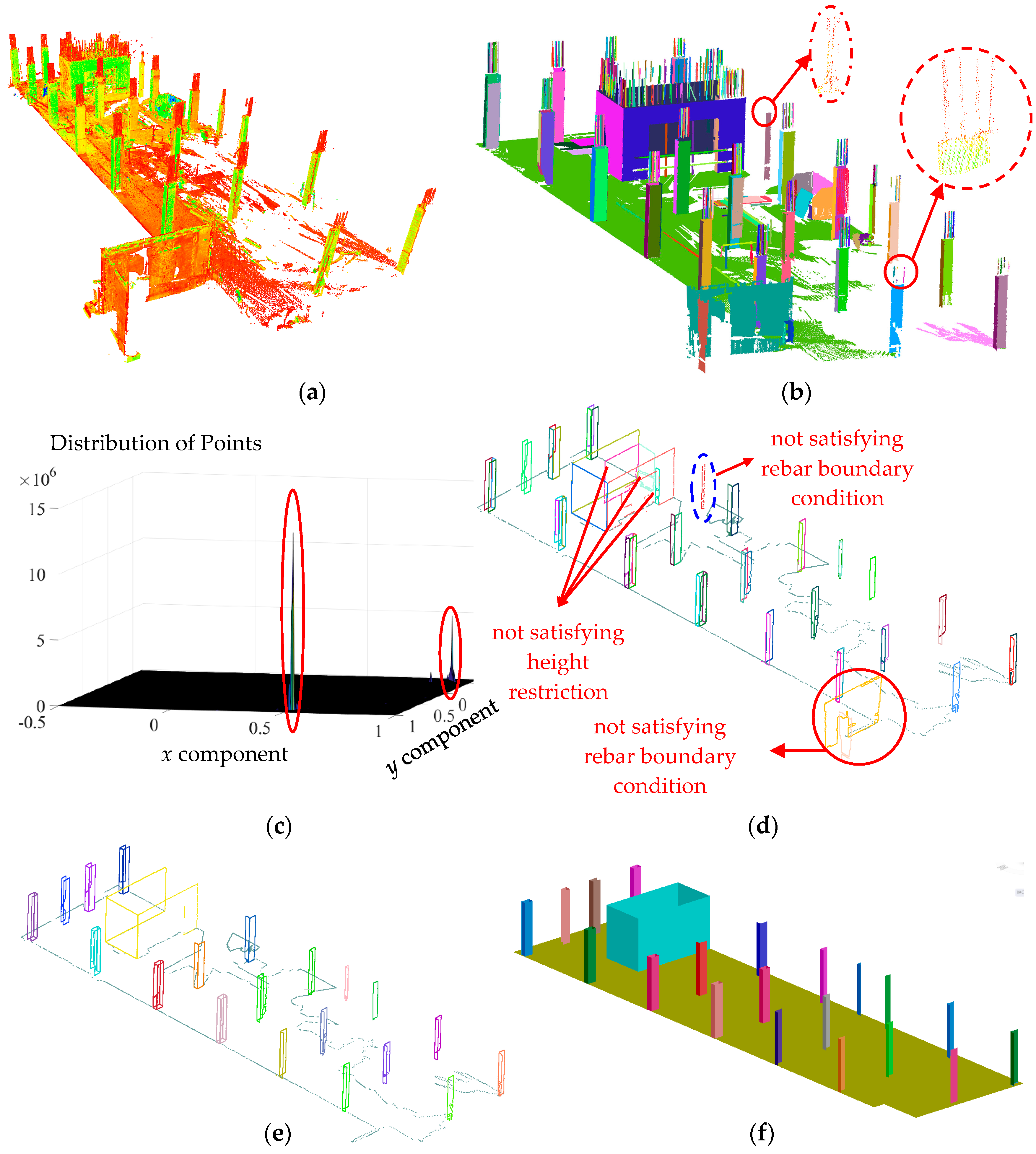
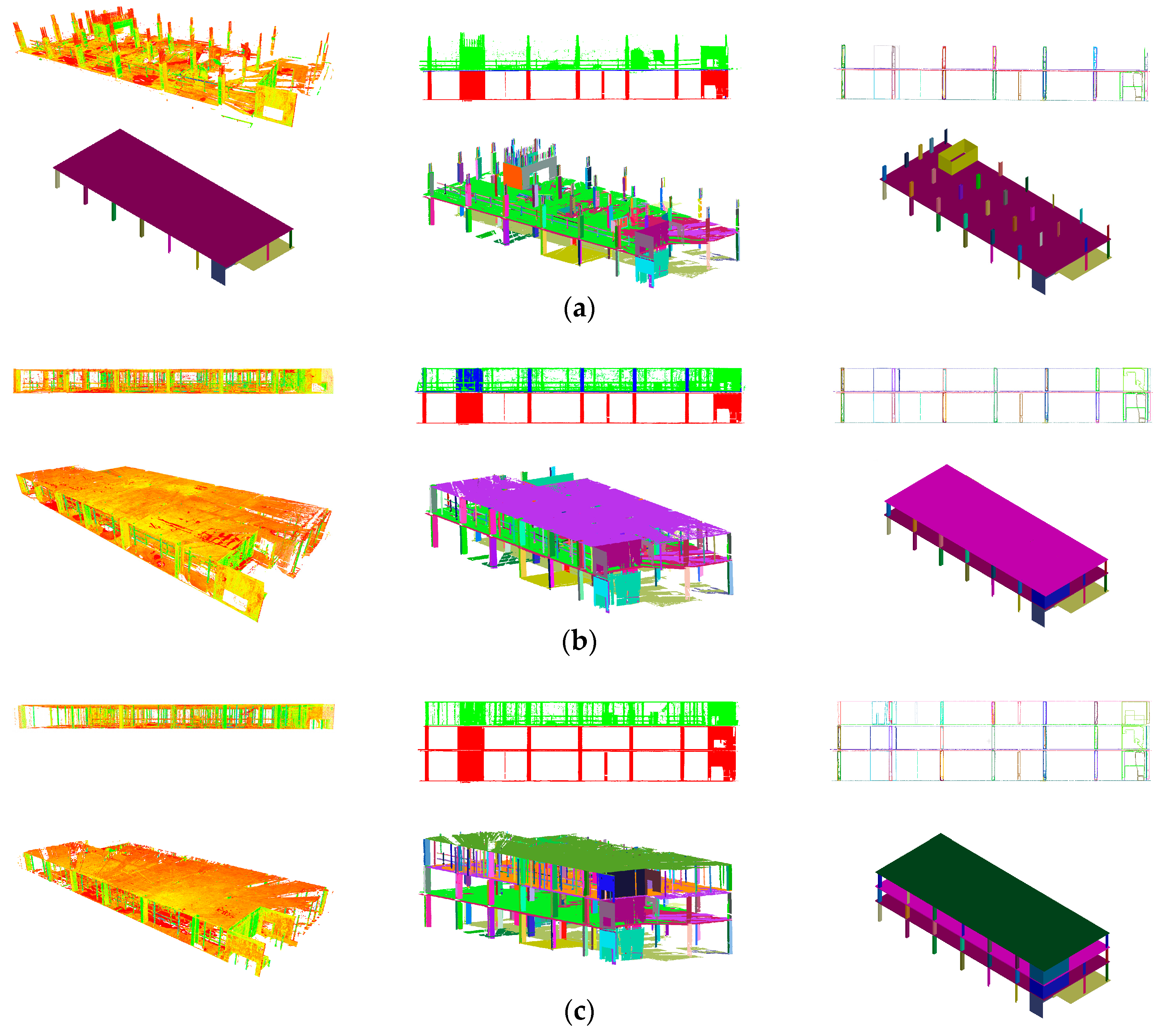
4.2. Extraction of Columns from Segmented Planar and Linear Features

The results of the planar and linear segmentation of the GSHR construction site using robust PCA classification and robust complete linkage segmentation were given in [22]. Here, the planar and linear segmentation results are used to extract structural columns through Algorithms 1 and 2. Figure 7a,b illustrates the point cloud and segmented planar and linear features for epoch 1. In Figure 7b, the red ovals represent two instances where the rebars were not effectively identified due to low point density of the collected data. As can be seen in Table 1, the scan resolution was increased after epoch 1 to collect more points and prevent the misclassification problem due to low point density [22].

Figure 7c shows the bivariate histogram of the x−y components of the normal vector of the identified planar surfaces. Illustrated in red ovals, the histogram consists of two main modes, which represent the planar surfaces corresponding to the columns. The two modes with the highest frequency satisfying the orthogonality criteria of Algorithm 1, Equations (1) and (2), were identified. To provide some perspective, the absolute value of the dot product of the two main axes was 0.0036 (Equation 2), whereas the threshold of Equation (1) was 0.035, almost an order of magnitude larger. The boundaries of the planar segments whose normal vectors comply with the identified modes (the final output of Algorithm 1) are presented in Figure 7d. Figure 7e shows the boundaries of the segmented columns after the application of Algorithm 2 (i.e., segments satisfying the height and boundary conditions). In Figure 7d, the planar surfaces that followed the main site axes but were unable to satisfy the height restriction or boundary conditions are also marked. The planar surface shown in the blue dashed oval is the same surface shown in Figure 7b, where low point density prevented the correct extraction of the rebars. Since the rebars were not extracted, the surface was incorrectly eliminated following Algorithm 2. This shows the importance of the point cloud density on the planar and linear segmentation results and consequently the column extraction procedure. Once the point density was increased (epochs 2 through 5), all surfaces representing columns were consistently extracted correctly. The results of the column extraction for all epochs is summarized in

Table 2. Precision, recall, and accuracy of the automated column extraction for each epoch.

Epoch	Precision	Recall	Accuracy
1	95.45	100.00	96.30
2	100.00	100.00	100.00
3	100.00	100.00	100.00
4	100.00	100.00	100.00
5	100.00	100.00	100.00
Overall	99.24	100.00	99.31

. As observed, the overall precision, recall, and accuracy for the presented column extraction is 99.24%, 100.00%, and 99.31%, respectively. The visual results of the column extraction for epochs 2 through 5 can be illustrated in Figure 8 and Figure 9.

4.3. Results of Redundant Surface Removal

The generated as-built model of the final set of extracted columns for epoch 1 is shown in Figure 7f. Approximately one week after epoch 1, epoch 2 was acquired from the construction site. Based on the project’s planned schedule, the ceiling and surrounding columns of the first floor were expected to be completed. Before the point cloud of epoch 2 was processed, Algorithms 4–6 were applied to remove possible redundant surfaces so that the remaining processes (planar segmentation and object extraction) would only be carried out on points of newly added components. The results of the redundant surface removal for epoch 2 are shown in Figure 8c. The newly added points, redundant points between epochs 1 and 2, and points available in epoch 1 but not covered in epoch 2 are shown in green, blue, and red colors, respectively.

The redundant points (shown in blue Figure 1, Figure 8 and Figure 9) are semantically labeled as the objects represented by the matched surface (e.g., column represented by a plane). The processes described in Section 3.2 and Section 3.3 are then only carried out for the newly added points (green points in Figure 1, Figure 8 and Figure 9). Figure 8e shows the output of Algorithm 1, i.e., the planar surfaces following the main orthogonal orientations of the site. Figure 8f shows the extracted columns, shown in different colors following the height and boundary conditions imposed by Algorithm 2. As shown in Table 2, all columns for epoch 2 were correctly extracted.

The results of the redundant surface removal as well as column extraction (Algorithms 1 through 3) for epochs 3 through 5 are shown in Figure 9.

Table 3. Precision, recall, and accuracy of the automated redundant surface extraction.

Epochs	Precision	Recall	Accuracy
1–2	97.44	98.70	98.04
2–3	95.71	97.10	99.38
3–4	97.16	97.71	96.09
4–5	96.70	97.78	99.65
Overall	97.09	98.04	98.79

presents the precision, recall, and accuracy of the redundant surface extraction algorithm for epochs 2 through 5. The redundant surface removal method achieved an overall precision, recall, and accuracy of 97.09%, 98.04%, and 98.79%, respectively. The recall rate shows that a very small percentage of the new points were incorrectly added to the presegmented surfaces of previous epochs. Upon closer examination, 95.2% of the new points that were incorrectly identified as redundant were points close to two intersecting planar surfaces, where one of the surfaces was not covered in the previous scan; hence, the point was assigned to the closest presegmented surface. The rest (4.8%) were outlier points, such as mixed pixels, commonly present in datasets acquired from construction sites that satisfied the conditions presented in Algorithms 4–6.

4.4. As-Built vs. Planned BIM Comparison

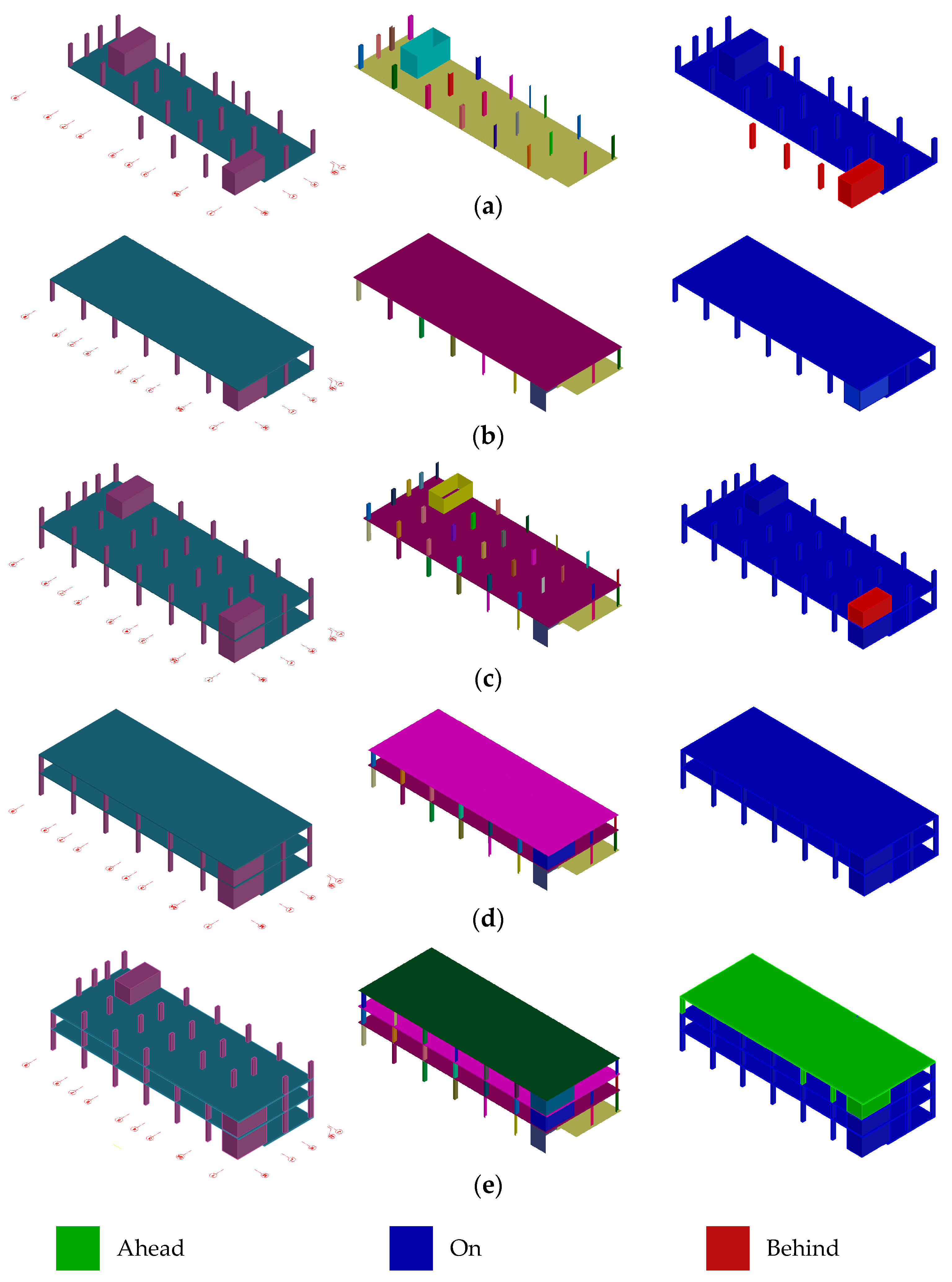
4.4.1. Progress Monitoring through EVM

Using the method described in Section 3.5, the corresponding elements between those planned and as-built were identified. Since the planned BIM did not contain 3D information related to the rebars, only the correspondence of columns and floor slabs were examined. Figure 10 (right) shows the result of the superimposition of the planned and the as-built elements. The object correspondences between the planned and as-built elements are visualized through color-coding. On-schedule, behind-schedule, and ahead-of-schedule objects are shown in blue, red, and green colors, respectively.

The colors presented in Figure 10 help with visual identification and reporting of the progress of specific construction elements (i.e., in activity level). To determine the performance of the whole project at each baseline, EVM is commonly employed [18]. Using the basic principles of EVM, the budgeted cost of work scheduled (BCWP), budgeted cost of work performed (BCWP), and schedule performance index (SPI) for each epoch were calculated. The result of the EVM is presented in

Table 4. Result of the earned value management to determine the project’s progress at each epoch.

Epochs	BCWS 1 (Units of Cost)	BCWP 2 (Units of Cost)	SPI 3	Schedule Performance of Project
1	1.73	1.29	0.74	Behind
2	2.56	2.56	1.00	On
3	3.62	3.35	0.93	Behind
4	4.18	4.18	1.00	On
5	4.90	5.57	1.14	Ahead

¹ Budgeted cost of work scheduled (BCWS), ² Budgeted cost of work performed (BCWP), ³ Schedule performance index (SPI).

. Using the calculated SPI, the schedule performance of the whole project at each epoch was determined (behind, ahead of, and on schedule). According to earned value analysis, SPI smaller than, equal to, or larger than 1 demonstrates that the project is behind, on, or ahead of schedule, respectively.

4.4.2. Dimensional Compliance Control

Since no information about the rebars’ placements was available in the planned BIM, only the conformity of the as-built dimensions of the columns and the slab thickness of those planned are presented. The planned cross-sectional dimensions of the columns (width and length) and thickness of the slabs were 350 mm, 600 mm, and 175 mm, respectively. The width and length of these columns as well as the slab thickness were also measured by means of a measuring tape as ground truth. Based on the information presented in [52], the tolerance of the cross section of a rectangular column with planned dimensions between 305 mm and 914 mm is between +13 mm and −10 mm (i.e., the column’s dimensions can exceed more than they can be reduced due to designed strength limitations). The tolerance of the thickness of the concrete slabs is ±6 mm. For each epoch, the DRMS [58] of the dimensions of the columns’ cross sections from those planned were calculated. The DRMS was also calculated for the estimated dimensions compared to ground truth measurements (dimensions obtained by measuring tape) for comparison. The results of the column dimensional compliance are presented in

Table 5. Accuracy assessment of column cross-section dimensions.

Epochs	DRMS 1 Compared to Planned (mm)	DRMS Compared to Ground Truth (mm)	Columns within Tolerance (%)
1	9	2	90.48
2	6	1	100.00
3	8	2	96.15
4	6	2	100.00
5	8	1	93.10
Overall	7	1	96.21

¹ Distance root mean squared (DRMS).

. The percentage of columns passing the cross-sectional tolerance criteria for each epoch is also provided in Table 5. A column is considered compliant if it satisfies the tolerance check criteria in both width and length. As illustrated, 96.21% of the columns (127 out of 132 identified columns) in all datasets complied with their planned dimensions (i.e., their cross-sectional dimensions were within +13 mm and −10 mm from the planned dimensions).

Accordingly, the difference in the slab thickness from the designed as well as the ground truth for floors 2 and 3 is calculated and presented in

Table 6. Accuracy assessment of floor slab thickness.

Floors	Estimated Slab Thickness (mm)	Absolute Difference from Plan (mm)	Absolute Difference from Ground Truth (mm)
2	173	2	0
3	179	4	1

. The first floor was on the ground (slab on grade), and hence, calculation of the slab thickness is not relevant. As illustrated, the thickness of the slab of both floors 2 and 3 are within 6 mm of the planned dimensions.

5. Summary of Findings and Discussion

The objective of the experiment was to assess the effectiveness of the column extraction and redundant point removal methods (Algorithms 1–6) in real-world point cloud data acquired from cast-in-place regular rectangular concrete construction. It was shown that 132 out of 133 columns were extracted correctly using Algorithms 1 and 2 as presented in the manuscript. In all five datasets, only one column was not correctly extracted. This was attributed to the low point density of the scan in epoch 1, preventing the linear classification and segmentation of [22] to identify the rebars on top of this particular column. Once the point density of the TLS instrument was increased for prospective scans, the column extraction was able to correctly extract the remaining columns consistently. The recall rate of the column extraction was 100%, which demonstrates the robustness of the method to type II errors (i.e., no other object was incorrectly identified as a column).

The redundant surface removal was also applied to epochs 2 through 5 with an overall precision, recall, and accuracy of 97.09%, 98.04%, and 98.79%, respectively. The recall rate suggests that only a small portion of the points of the new scan was incorrectly identified as redundant. Upon closer examination, it was observed that 95.2% of the incorrectly classified points were points of an adjacent surface where the surface was not covered in the previous scan.

The success of the algorithms in the removal of redundant as well as the semantic labeling of points enabled the automatic comparison of as-built vs. planned elements. Here, two applications, namely progress monitoring as well as dimensional compliance control, using the proposed methods, were presented. It was shown that the system identified and visualized the progress of construction work in activity level, which is one of the limitations of current progress-monitoring practices in the industry [60]. It was also shown that the produced results can be used to determine the performance of the whole project at a given baseline using some project controls method, such as EVM.

The as-built dimensions of the cross section of the rectangular columns and the thickness of the floor slabs were compared to that of the planned to determine potential dimensional discrepancies. It was shown that the thickness of the flat slabs of floors 2 and 3 complied with the planned dimensions (i.e., within standard tolerances). It was also shown that 127 out of the 132 identified columns were also within the acceptable tolerances from their planned dimensions. The ground truth of the dimensions of the columns and slabs was collected using a measuring tape to a millimeter precision. The DRMS of all the dimensions of columns to the ground truth was approximately 1 mm, which shows good agreement since most quality standards in industrial construction allow up to 5 mm deviation in each direction [8].

6. Conclusions

This manuscript provides a robust framework for the semantic labeling of common reinforced structural concrete components from unorganized point clouds acquired at regular rectangular buildings during construction. The framework first classifies and segments registered point clouds into planar and linear features using robust PCA, Monte Carlo simulation, and the robust variation of the complete linkage hierarchical clustering method, as proposed by [22]. Columns, floors, and rebars are then extracted through relationship-based reasoning derived from the specific characteristics of reinforced concrete structures and regular rectangular buildings. The framework also incorporates a novel redundant point removal method to remove points of prospective scans that were classified into objects in previous scans.

Five sets of point cloud data were acquired from the GSHR construction site at the University of Calgary to assess the effectiveness of the proposed methods for semantic labeling and redundant point removal. The results substantiated the effectiveness and the ability of the column extraction to extract 132 out of 133 columns in all datasets with an overall object extraction accuracy of 99.31%. The redundant point removal also achieved an overall extraction accuracy of 98.79%, which demonstrates its applicability in redundant point removal of point clouds acquired from construction sites.

Two applications, namely progress monitoring and dimensional quality control, of the proposed column extraction and redundant point removal were presented. It was observed that these methods enable the automated color-coding for visual representation of progress in activity level. An EVM was also carried out to determine the overall project’s performance at each epoch. The dimensions of the extracted columns and slabs were also compared to the planned and ground truth. It was shown that 127 out of the identified 132 columns and both floor slabs (levels 2 and 3) passed the tolerance criteria set within the standard code for concrete structures.

The methods presented in this manuscript showed great promise for the automated extraction of common structural elements from reinforced concrete structures with applications to automated progress monitoring and dimensional compliance control. The following provide additional avenues for future research and expansion:

• Examination of the methods proposed in this manuscript for progress monitoring and dimensional conformity control of rebars in reinforced concrete projects where a detailed planned BIM, containing the complete details of the rebars, exists.
• The simultaneous application of scan vs. BIM, supervised learning, and the methods proposed in our study for the extraction of structural components with complex geometries. Additionally, the application of novel methods used to reduce the dependency of semantic labeling on new training data, such as those presented in [61], for TLS acquired from construction sites is an interesting research topic for future investigations.
• The extraction of temporary objects, such as scaffolds and formwork, from TLS acquired from construction sites using validated methods applied to photogrammetric point clouds, such as those proposed in [62].
• Evaluations of methods proposed by [63] for surface flatness assessment to generate a standardized surface flatness metric.
• Development of a fuzzy logic-based uncertainty model for the estimation of the location of structures, similar to the method proposed by [64] for the prediction of the locations of utility data.

References

- Josephson, P.E.; Larsson, B.; Li, H. Illustrative Benchmarking Rework and Rework Costs in Swedish Construction Industry. J. Manag. Eng. 2002, 18, 76–83. [Google Scholar] [CrossRef]
- Oko, J.A.; Itodo, E.D. Professionals’ Views of Material Wastage on Construction Sites and Cost Overruns. Organ. Technol. Manag. Constr. Int. J. 2013, 5, 747–757. [Google Scholar] [CrossRef]
- Kultermann, E.; Spence, W.P. Construction Materials, Methods and Techniques, 4th ed.; Cengage Learning: Boston, MA, USA, 2016; ISBN 978-1-3050-8627-2. [Google Scholar]
- Geng, Y.; Wang, Z.; Shen, L.; Zhao, J. Calculating of CO2 Emission Factors for Chinese Cement Production Based on Inorganic Carbon and Organic Carbon. J. Clean. Prod. 2019, 217, 503–509. [Google Scholar] [CrossRef]
- Miami Herald: Feds Fine Contractors Behind Deadly FIU Bridge Collapse for ‘Serious’ Safety Violations. Available online: https://www.miamiherald.com/news/local/community/miami-dade/article218594530.html (accessed on 11 April 2019).
- Shalabi, F.; Turkan, Y. IFC BIM-Based Facility Management Approach to Optimize Data Collection for Corrective Maintenance. J. Perform. Constr. Facil. 2017, 31, 04016081. [Google Scholar] [CrossRef]
- Jalaei, F.; Zoghi, M.; Khoshand, A. Life Cycle Environmental Impact Assessment to Manage and Optimize Construction Waste Using Building Information Modeling (BIM). Int. J. Constr. Manag. 2019, 1–18. [Google Scholar] [CrossRef]
- Maalek, R.; Lichti, D.D.; Walker, R.; Bhavnani, A.; Ruwanpura, J.Y. Extraction of Pipes and Flanges from Point Clouds for Automated Verification of PreFabricated Modules in Oil and Gas Refinery Projects. Autom. Constr. 2019, 103, 150–167. [Google Scholar] [CrossRef]
- Tang, P.; Huber, D.; Akinci, B.; Lipman, R.; Lytle, A. Automatic Reconstruction of As-Built Building Information Models from Laser-Scanned Point Clouds: A Review of Related Techniques. Autom. Constr. 2010, 19, 829–843. [Google Scholar] [CrossRef]
- Son, H.; Bosché, F.; Kim, C. As-Built Data Acquisition and Its Use in Production Monitoring and Automated Layout of Civil Infrastructure: A Survey. Adv. Eng. Inform. 2015, 29, 172–183. [Google Scholar] [CrossRef]
- Pătrăucean, V.; Armeni, I.; Nahangi, M.; Yeung, J.; Brilakis, I.; Haas, C. State of Research in Automatic As-Built Modelling. Adv. Eng. Inform. 2015, 29, 162–171. [Google Scholar] [CrossRef]
- Lehtola, V.V.; Kaartinen, H.; Nüchter, A.; Kaijaluoto, R.; Kukko, A.; Litkey, P.; Honkavaara, E.; Rosnell, T.; Vaaja, M.T.; Virtanen, J.-P.; et al. Comparison of the Selected State-Of-The-Art 3D Indoor Scanning and Point Cloud Generation Methods. Remote Sens. 2017, 9, 796. [Google Scholar] [CrossRef]
- Wang, R.; Peethambaran, J.; Chen, D. LiDAR Point Clouds to 3-D Urban Models: A Review. IEEE J. Sel. Top. Appl. Earth Obs. Remote Sens. 2018, 11, 606–627. [Google Scholar] [CrossRef]
- Wang, Q.; Tan, Y.; Mei, Z. Computational Methods of Acquisition and Processing of 3D Point Cloud Data for Construction Applications. Arch. Comput. Methods Eng. 2019. [Google Scholar] [CrossRef]
- Bosche, F.; Haas, C.T. Automated Retrieval of 3D CAD Model Objects in Construction Range Images. Autom. Constr. 2008, 17, 499–512. [Google Scholar] [CrossRef]
- Bosché, F. Automated Recognition of 3D CAD Model Objects in Laser Scans and Calculation of As-Built Dimensions for Dimensional Compliance Control in Construction. Adv. Eng. Inform. 2010, 24, 107–118. [Google Scholar] [CrossRef]
- Bosché, F.; Guillemet, A.; Turkan, Y.; Haas, C.T.; Haas, R. Tracking the Built Status of MEP Works: Assessing the Value of a Scan-vs-BIM System. J. Comput. Civ. Eng. 2014, 28, 05014004. [Google Scholar] [CrossRef]
- Turkan, Y.; Bosche, F.; Haas, C.T.; Haas, R. Automated Progress Tracking Using 4D Schedule and 3D Sensing Technologies. Autom. Constr. 2012, 22, 414–421. [Google Scholar] [CrossRef]
- Kim, C.; Son, H.; Kim, C. Automated Construction Progress Measurement Using a 4D Building Information Model and 3D Data. Autom. Constr. 2013, 31, 75–82. [Google Scholar] [CrossRef]
- Turkan, Y.; Bosché, F.; Haas, C.T.; Haas, R. Tracking of Secondary and Temporary Objects in Structural Concrete Work. Constr. Innov. 2014, 14, 145–167. [Google Scholar] [CrossRef]
- Zhang, C.; Arditi, D. Automated Progress Control Using Laser Scanning Technology. Autom. Constr. 2013, 36, 108–116. [Google Scholar] [CrossRef]
- Maalek, R.; Lichti, D.D.; Ruwanpura, J.Y. Robust Segmentation of Planar and Linear Features of Terrestrial Laser Scanner Point Clouds Acquired from Construction Sites. Sensors 2018, 18, 819. [Google Scholar] [CrossRef]
- Yang, J.; Shi, Z.-K.; Wu, Z.-Y. Towards Automatic Generation of As-Built BIM: 3D Building Facade Modeling and Material Recognition from Images. Int. J. Autom. Comput. 2016, 13, 338–349. [Google Scholar] [CrossRef]
- Kim, H.; Kim, K.; Kim, H. Data-Driven Scene Parsing Method for Recognizing Construction Site Objects in the Whole Image. Autom. Constr. 2016, 71, 271–282. [Google Scholar] [CrossRef]
- Verity—Clear Edge 3D. Available online: http://www.clearedge3d.com/products/verity/ (accessed on 11 April 2019).
- Chai, J.; Chi, H.-L.; Wang, X.; Wu, C.; Jung, K.H.; Lee, J.M. Automatic As-Built Modeling for Concurrent Progress Tracking of Plant Construction Based on Laser Scanning. Concurr. Eng. 2016, 24, 369–380. [Google Scholar] [CrossRef]
- Son, H.; Kim, C. Semantic As-Built 3D Modeling of Structural Elements of Buildings Based on Local Concavity and Convexity. Adv. Eng. Inform. 2017, 34, 114–124. [Google Scholar] [CrossRef]
- Xiong, X.; Adan, A.; Akinci, B.; Huber, D. Automatic Creation of Semantically Rich 3D Building Models from Laser Scanner Data. Autom. Constr. 2013, 31, 325–337. [Google Scholar] [CrossRef]
- Rabbani, T.; van den Heuvel, F.A.; Vosselman, G. Segmentation of Point Clouds Using Smoothness Constraints. In ISPRS 2006: Proceedings of the ISPRS Commission V Symposium Vol. 35, Part 6: Image Engineering and Vision Metrology, Dresden, Germany, 25–27 September 2006; International Society for Photogrammetry and Remote Sensing (ISPRS): Dresden, Germany, 2006; pp. 248–253. Available online: https://www.isprs.org/proceedings/XXXVI/part5/paper/RABB_639.pdf (accessed on 8 May 2019).
- Wolpert, D.H. Stacked Generalization. Neural Netw. 1992, 5, 241–259. [Google Scholar] [CrossRef]
- Czerniawski, T.; Sankaran, B.; Nahangi, M.; Haas, C.; Leite, F. 6D DBSCAN-Based Segmentation of Building Point Clouds for Planar Object Classification. Autom. Constr. 2018, 88, 44–58. [Google Scholar] [CrossRef]
- Schnabel, R.; Wahl, R.; Klein, R. Efficient RANSAC for Point-Cloud Shape Detection. Comput. Graph. Forum 2007, 26, 214–226. [Google Scholar] [CrossRef]
- Ester, M.; Kriegel, H.-P.; Xu, X. A density-based algorithm for discovering clusters in large spatial databases with noise. In Proceedings of the Second International Conference on Knowledge Discovery and Data Mining, KDD’96, Portland, OR, USA, 2–4 August 1996; pp. 226–231. [Google Scholar]
- Son, H.; Kim, C.; Hwang, N.; Kim, C.; Kang, Y. Classification of Major Construction Materials in Construction Environments Using Ensemble Classifiers. Adv. Eng. Inform. 2014, 28, 1–10. [Google Scholar] [CrossRef]
- Ma, L.; Sacks, R.; Kattel, U.; Bloch, T. 3D Object Classification Using Geometric Features and Pairwise Relationships. Comput.-Aided Civ. Infrastruct. Eng. 2018, 33, 152–164. [Google Scholar] [CrossRef]
- Shi, W.; Ahmed, W.; Li, N.; Fan, W.; Xiang, H.; Wang, M. Semantic Geometric Modelling of Unstructured Indoor Point Cloud. ISPRS Int. J. Geo-Inf. 2019, 8, 9. [Google Scholar] [CrossRef]
- Macher, H.; Landes, T.; Grussenmeyer, P. From Point Clouds to Building Information Models: 3D Semi-Automatic Reconstruction of Indoors of Existing Buildings. Appl. Sci. 2017, 7, 1030. [Google Scholar] [CrossRef]
- Pu, S.; Vosselman, G. Knowledge Based Reconstruction of Building Models from Terrestrial Laser Scanning Data. ISPRS J. Photogramm. Remote Sens. 2009, 64, 575–584. [Google Scholar] [CrossRef]
- Vosselman, G.; Gorte, B.G.H.; Sithole, G.; Rabbani, T. Recognising Structure in Laser Scanning Point Clouds. In Proceedings of the ISPRS Working Group VIII/2: Laser Scanning for Forest and Landscape Assessment, ISPRS 2004, Freiburg, Germany, 3–6 October 2004; University of Freiburg: Freiburg, Germany, 2004; pp. 33–38. [Google Scholar]
- Wang, Q.; Yan, L.; Zhang, L.; Ai, H.; Lin, X. A Semantic Modelling Framework-Based Method for Building Reconstruction from Point Clouds. Remote Sens. 2016, 8, 737. [Google Scholar] [CrossRef]
- Hong, S.; Jung, J.; Kim, S.; Cho, H.; Lee, J.; Heo, J. Semi-Automated Approach to Indoor Mapping for 3D as-Built Building Information Modeling. Comput. Environ. Urban Syst. 2015, 51, 34–46. [Google Scholar] [CrossRef]
- Ochmann, S.; Vock, R.; Klein, R. Automatic Reconstruction of Fully Volumetric 3D Building Models from Oriented Point Clouds. ISPRS J. Photogramm. Remote Sens. 2019, 151, 251–262. [Google Scholar] [CrossRef]
- Maalek, R.; Lichti, D.D.; Ruwanpura, J. Robust Classification and Segmentation of Planar and Linear Features for Construction Site Progress Monitoring and Structural Dimension Compliance Control. ISPRS Ann. Photogramm. Remote Sens. Spat. Inf. Sci. 2015, 3, 129–136. [Google Scholar] [CrossRef]
- Li, L.; Su, F.; Yang, F.; Zhu, H.; Li, D.; Zuo, X.; Li, F.; Liu, Y.; Ying, S. Reconstruction of Three-Dimensional (3D) Indoor Interiors with Multiple Stories via Comprehensive Segmentation. Remote Sens. 2018, 10, 1281. [Google Scholar] [CrossRef]
- Díaz-Vilariño, L.; Conde, B.; Lagüela, S.; Lorenzo, H. Automatic Detection and Segmentation of Columns in As-Built Buildings from Point Clouds. Remote Sens. 2015, 7, 15651–15667. [Google Scholar] [CrossRef]
- Steadman, P. Why Are Most Buildings Rectangular? ARQ Archit. Res. Q. 2006, 10, 119–130. [Google Scholar] [CrossRef]
- Nunnally, S.W. Construction Methods and Management, 8th ed.; Pearson Education: Upper Saddle River, NJ, USA, 2010; pp. 517–518. [Google Scholar]
- Zalka, K.A. Structural Analysis of Regular Multi-Storey Buildings, 1st ed.; CRC Press: Boca Raton, FL, USA, 2012. [Google Scholar]
- Fukunaga, K.; Hostetler, L. The Estimation of the Gradient of a Density Function, with Applications in Pattern Recognition. IEEE Trans. Inf. Theory 1975, 21, 32–40. [Google Scholar] [CrossRef]
- Shimazaki, H.; Shinomoto, S. Kernel Bandwidth Optimization in Spike Rate Estimation. J. Comput. Neurosci. 2010, 29, 171–182. [Google Scholar] [CrossRef]
- ACI Committee 117. Specification for Tolerances for Concrete Construction and Materials (Reapproved 2015); American Concrete Institute: Farmington Hills, MI, USA, 2010. [Google Scholar]
- Ballast, D.K. Handbook of Construction Tolerances, 2nd ed.; John Wiley & Sons: Hoboken, NJ, USA, 2007. [Google Scholar]
- Edelsbrunner, H.; Kirkpatrick, D.; Seidel, R. On the Shape of a Set of Points in the Plane. IEEE Trans. Inf. Theory 1983, 29, 551–559. [Google Scholar] [CrossRef]
- Fayed, M.; Mouftah, H.T. Localised Alpha-Shape Computations for Boundary Recognition in Sensor Networks. Ad Hoc Netw. 2009, 7, 1259–1269. [Google Scholar] [CrossRef]
- ACI Committee 318. Building Code Requirements for Structural Concrete; American Concrete Institute: Farmington Hills, MI, USA, 2014. [Google Scholar]
- Sampath, A.; Shan, J. Building Boundary Tracing and Regularization from Airborne Lidar Point Clouds. Photogramm. Eng. Remote Sens. 2007, 73, 805–812. [Google Scholar] [CrossRef]
- Olsen, D.L.; Denlen, D. Advanced Data Mining Techniques; Springer: New York, NY, USA, 2008; p. 138. [Google Scholar]
- Maalek, R.; Sadeghpour, F. Accuracy Assessment of Ultra-Wide Band Technology in Tracking Static Resources in Indoor Construction Scenarios. Autom. Constr. 2013, 30, 170–183. [Google Scholar] [CrossRef]
- Leica HDS6100 TLS Datasheet and Key Performance Specifications. Available online: http://w3.leicageosystems.com/downloads123/hds/hds/HDS6100/brochures/Leica_HDS6100_brochure_us.pdf (accessed on 29 April 2019).
- Maalek, R.; Ruwanpura, J.; Ranaweera, K. Evaluation of the State-of-the-Art Automated Construction Progress Monitoring and Control Systems. In Construction Research Congress 2014; American Society of Civil Engineers: Atlanta, GA, USA, 2014; pp. 1023–1032. [Google Scholar] [CrossRef]
- Wu, J.; Yao, W.; Zhang, J.; Li, Y. 3D Semantic Labeling of ALS Data Based on Domain Adaption by Transferring and Fusing Random Forest Models. ISPRS Int. Arch. Photogramm. Remote Sens. Spat. Inf. Sci. 2018, XLII-3, 1883–1887. [Google Scholar] [CrossRef]
- Xu, Y.; Tuttas, S.; Hoegner, L.; Stilla, U. Reconstruction of Scaffolds from a Photogrammetric Point Cloud of Construction Sites Using a Novel 3D Local Feature Descriptor. Autom. Constr. 2018, 85, 76–95. [Google Scholar] [CrossRef]
- Bosché, F.; Guenet, E. Automating Surface Flatness Control Using Terrestrial Laser Scanning and Building Information Models. Autom. Constr. 2014, 44, 212–226. [Google Scholar] [CrossRef]
- Olde Scholtenhuis, L.L.; den Duijn, X.; Zlatanova, S. Representing Geographical Uncertainties of Utility Location Data in 3D. Autom. Constr. 2018, 96, 483–493. [Google Scholar] [CrossRef]