Detecting Forest Disturbance and Recovery in Primorsky Krai, Russia, Using Annual Landsat Time Series and Multi–Source Land Cover Products


Abstract
:
1. Introduction
- Is it possible to extend a forest change detection algorithm and parameter system to make them suitable for the Russian Far East based on the LandTrendr algorithm?
- What is the forest change trend in Primorsky Krai, Russia, over the past 18 years?
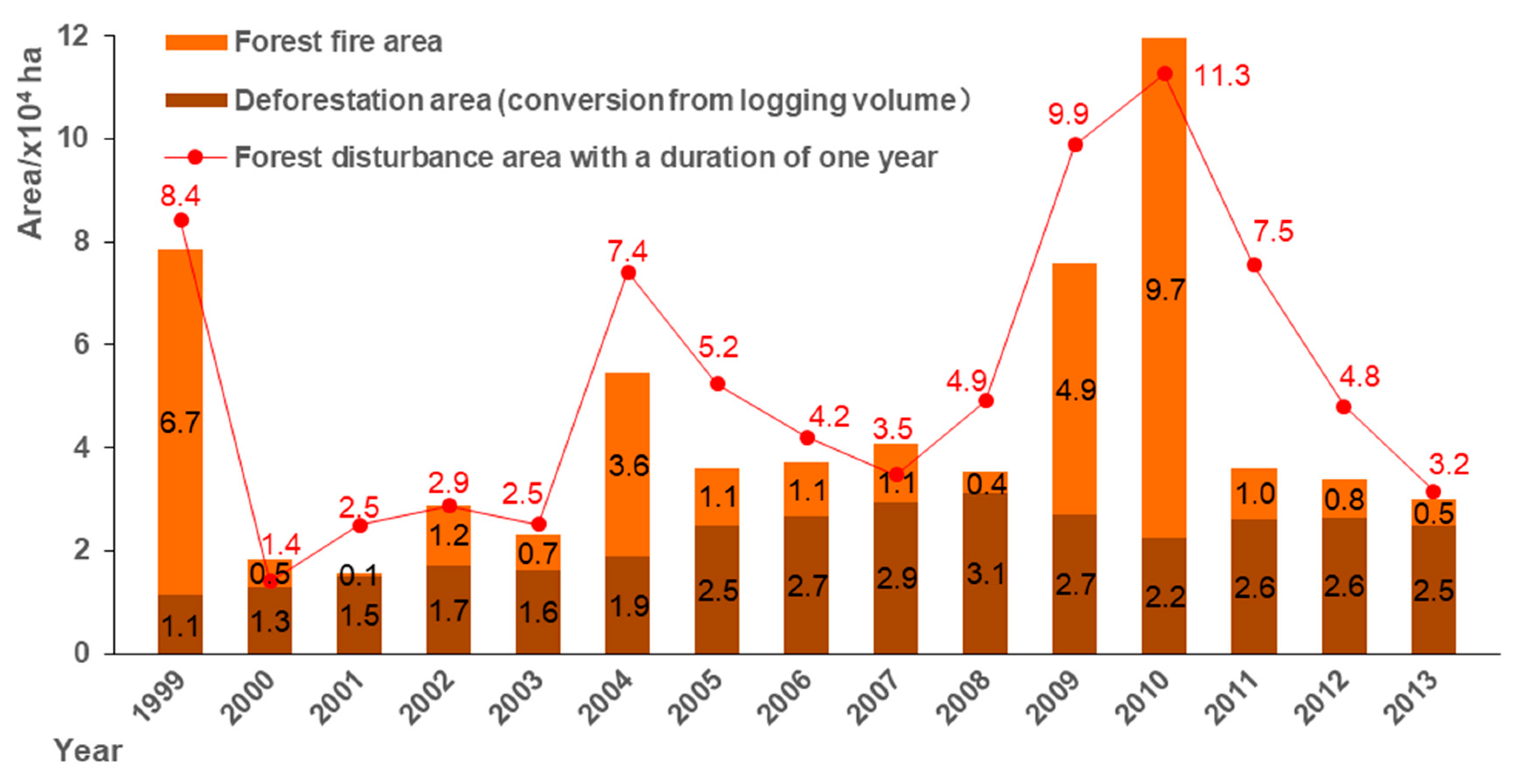
- What is the relationship between forest change (especially forest disturbance) and regional physical geography and economic and societal development?
2. Data and Methods
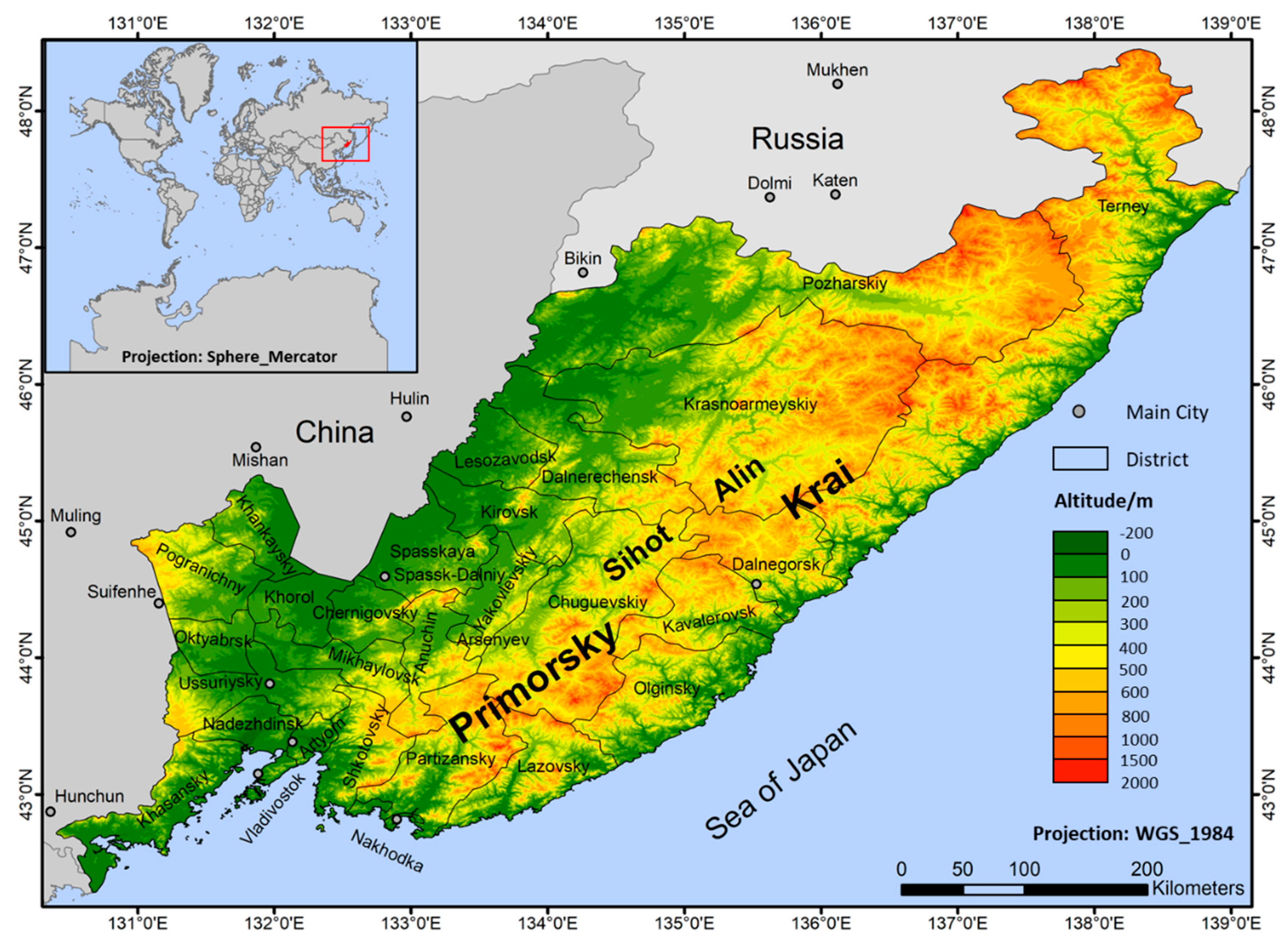
2.1. Research Area
2.2. Basic Data
2.3. Forest Change Mapping
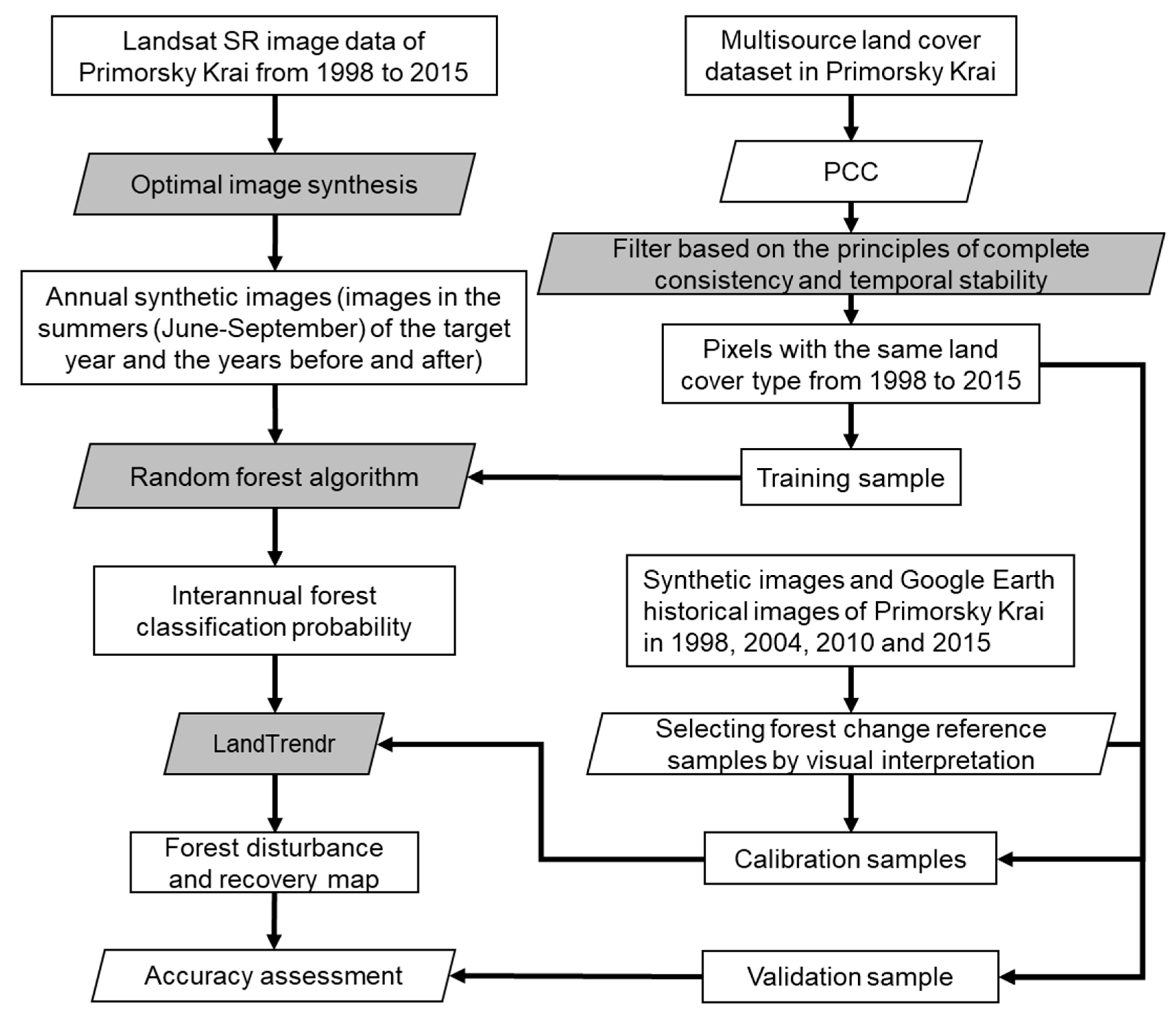
2.3.1. Overall Technical Process
- The best pixel synthesis method was applied, and Landsat SR synthetic images with no clouds and no shadows from 1998 to 2015 in the research area were constructed from the massive image library provided by the GEE. See Section 2.3.2 for the specific methods.
- Based on four classic LULC products, i.e., MCD12Q1, CCI, GlobalLand30, and FROM–GLC, training and calibration samples were determined according to the principles of complete consistency and temporal stability of the pixel attributes (i.e., land type attributes) [27,44]. The specific method is described in Section 2.3.3.
- The RF classification method was applied to classify the yearly images from 1998 to 2015 and to obtain yearly and pixel–by–pixel forest–type probability values. The specific method is provided in Section 2.3.4.
- The LandTrendr algorithm was used to perform time–series segmentation on the yearly and pixel–by–pixel forest–type probability sequences obtained in the previous step. Through repeated comparison experiments, the key time–series segmentation parameters were determined. The specific method is described in Section 2.3.5.
2.3.2. Preparation of Time–Series Satellite Imagery
2.3.3. Selecting the Training and Validation Samples
2.3.4. Random Forest Classification
2.3.5. Determining the Forest Classification and Change Thresholds
3. Results
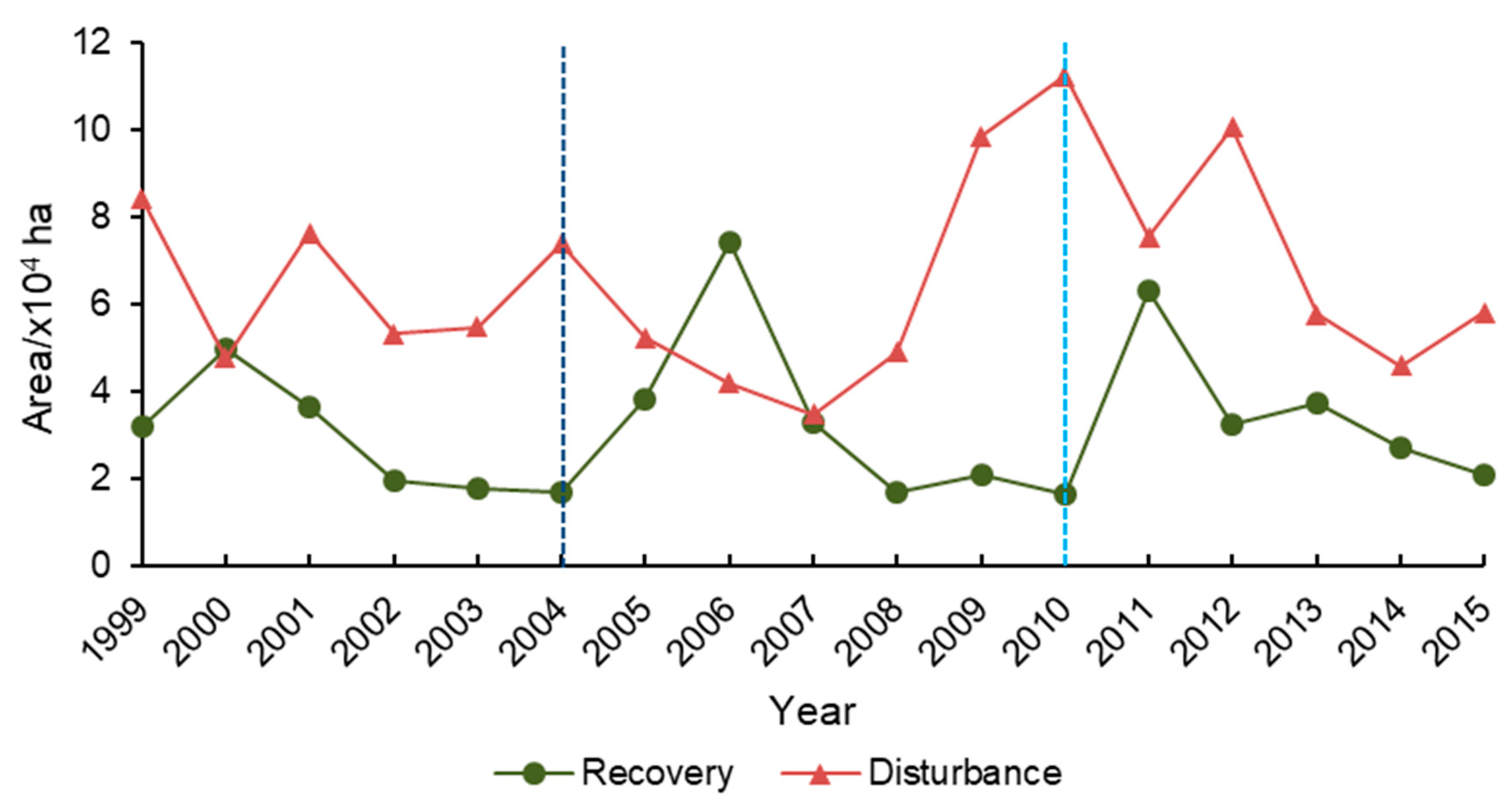
3.1. Quantitative Characteristics of Forest Change
3.2. Accuracy Assessment
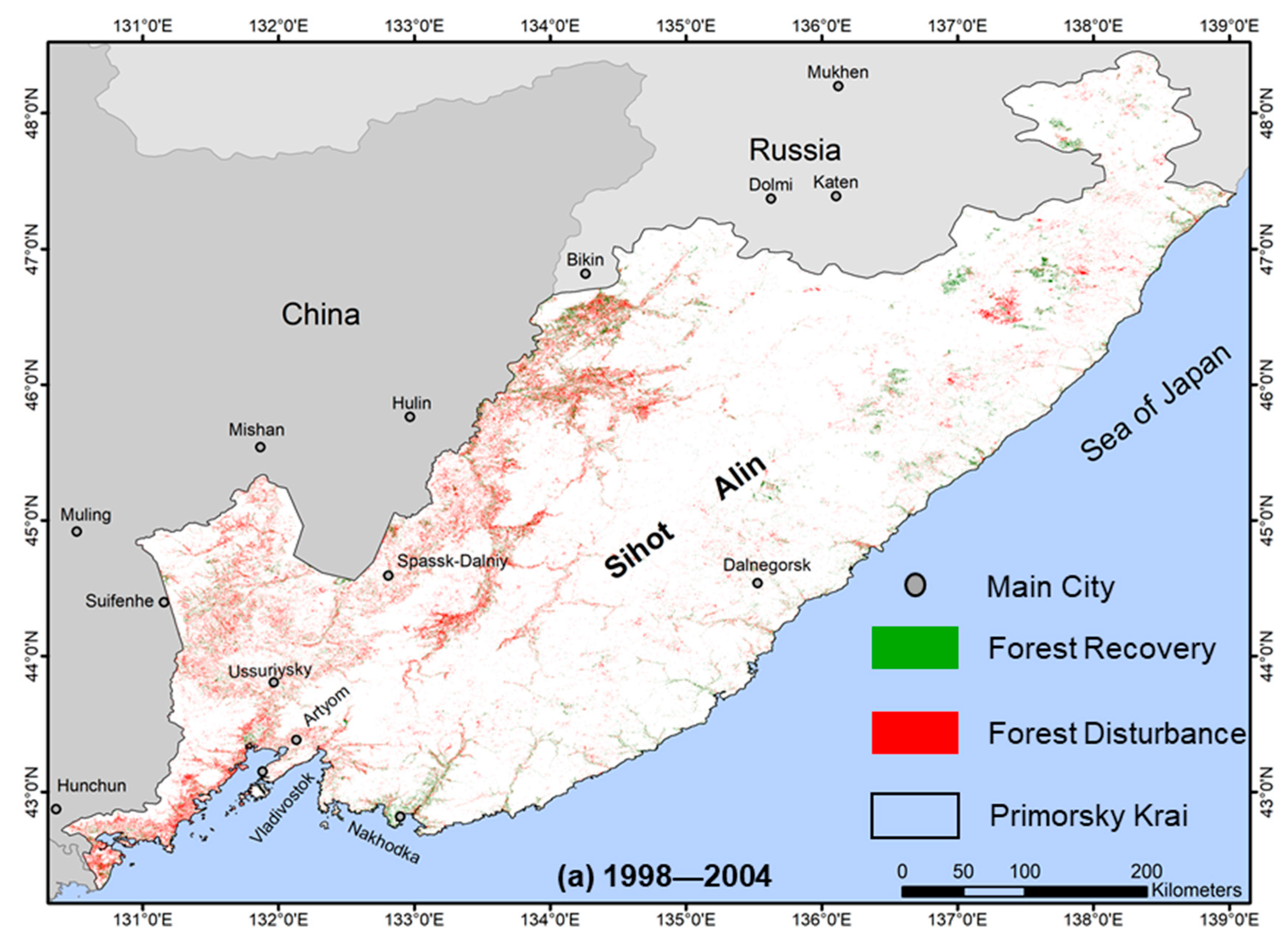
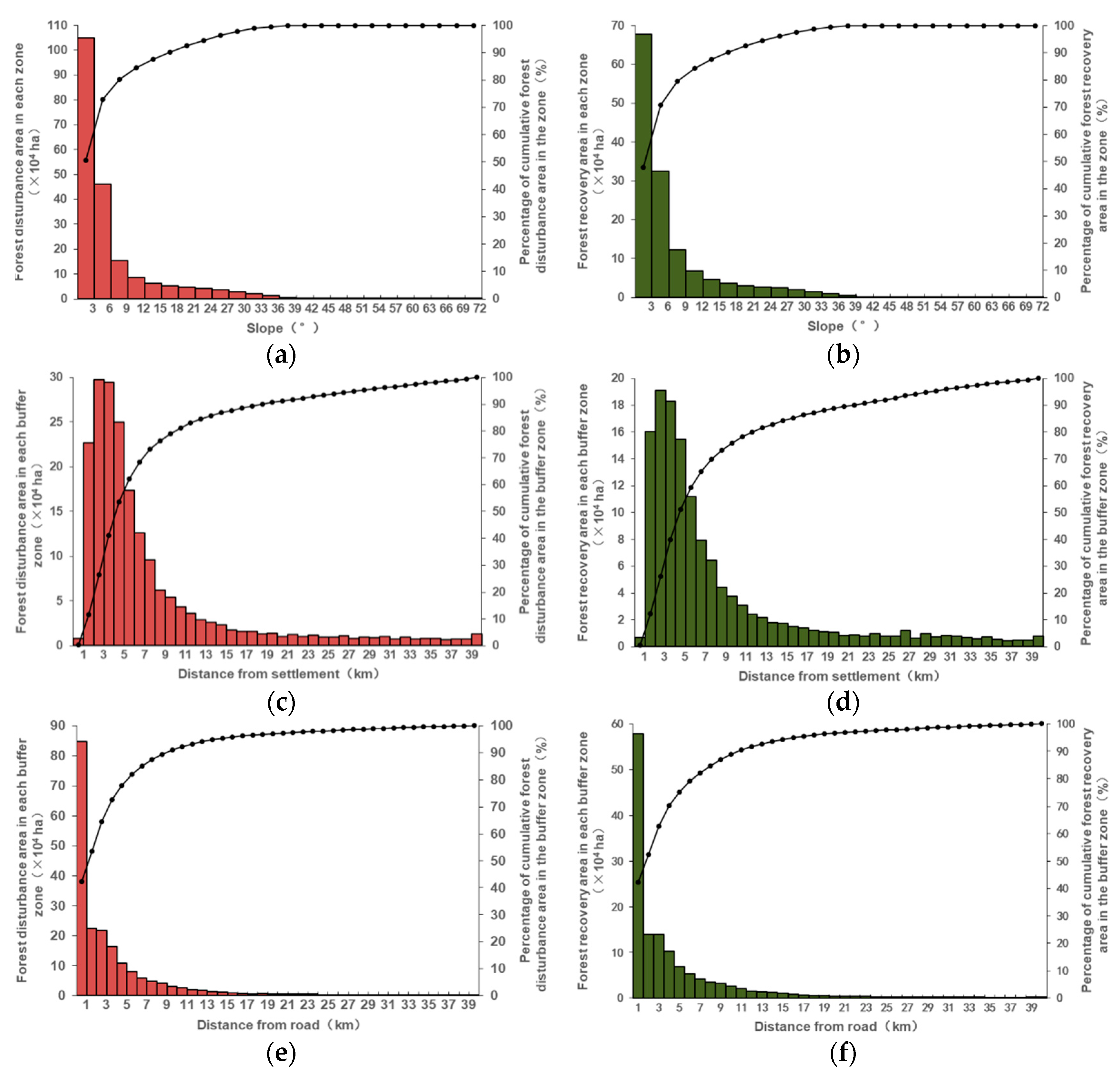
3.3. Spatial Characteristics of Forest Disturbance and Recovery
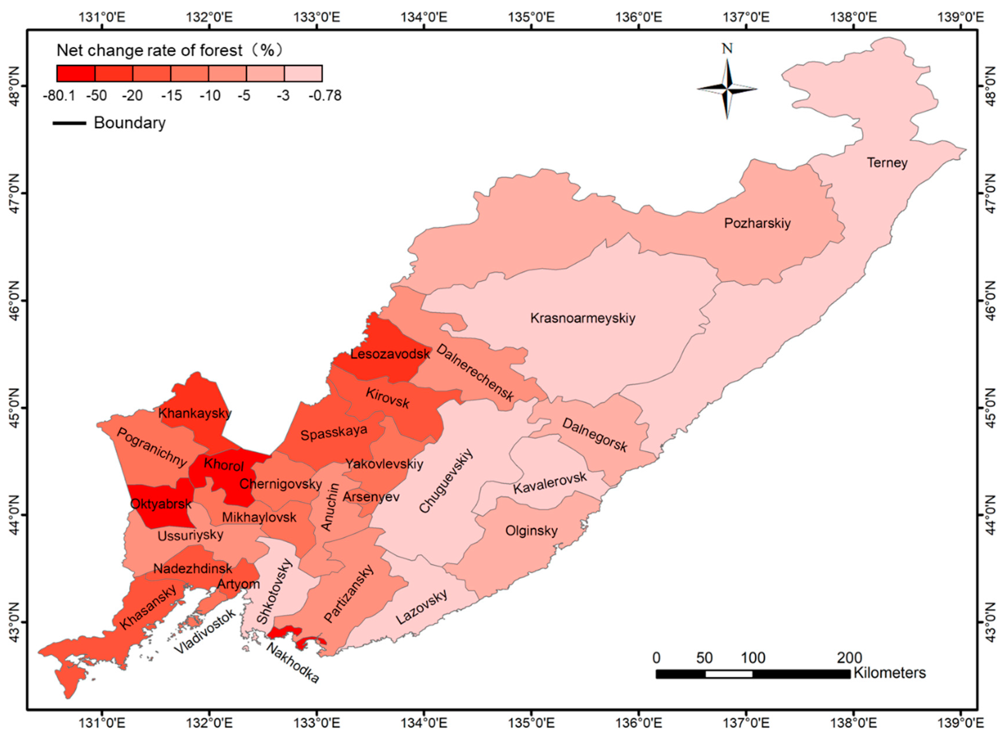
3.4. Spatial Distribution Pattern of the Net Forest Change
4. Discussion
4.1. New Discoveries and Their Potential Applications
4.2. Uncertainties of the Forest Change Detection Algorithm
5. Conclusions
Supplementary Materials
Author Contributions
Funding
Acknowledgments
Conflicts of Interest
References
- Dixon, R.K.; Solomon, A.M.; Brown, S.; Houghton, R.A.; Trexier, M.C.; Wisniewski, J. Carbon Pools and Flux of Global Forest Ecosystems. Science 1994, 263, 185–190. [Google Scholar] [CrossRef] [PubMed]
- Bonan, G.B. Forests and Climate Change: Forcings, Feedbacks, and the Climate Benefits of Forests. Science 2008, 320, 1444–1449. [Google Scholar] [CrossRef] [PubMed] [Green Version]
- Liu, S.; Wei, X.; Li, D.; Lu, D. Examining Forest Disturbance and Recovery in the Subtropical Forest Region of Zhejiang Province Using Landsat Time-Series Data. Remote Sens. 2017, 9, 479. [Google Scholar] [CrossRef] [Green Version]
- Desclée, B.; Bogaert, P.; Defourny, P. Forest change detection by statistical object-based method. Remote Sens. Environ. 2006, 102, 1–11. [Google Scholar] [CrossRef]
- Turner, D.P.; Ritts, W.D.; Kennedy, R.E.; Gray, A.N.; Yang, Z. Effects of harvest, fire, and pest/pathogen disturbances on the West Cascades ecoregion carbon balance. Carbon Balance Manag. 2015, 10, 12. [Google Scholar] [CrossRef] [Green Version]
- Houghton, R.A. Aboveground Forest Biomass and the Global Carbon Balance. Glob. Chang. Biol. 2010, 11, 945–958. [Google Scholar] [CrossRef]
- Yanping, L. A Survey of Russia’s Primorskij Kraj. Dong Jiang J. 2001, 18, 37–40. [Google Scholar]
- Vandergert, P.; Newell, J. Illegal logging in the Russian far east and Siberia. Int. For. Rev. 2003, 5, 303–306. [Google Scholar] [CrossRef] [Green Version]
- Loboda, T.V.; Zhang, Z.; O’Neal, K.J.; Sun, G.; Csiszar, I.A.; Shugart, H.H.; Sherman, N.J. Reconstructing disturbance history using satellite-based assessment of the distribution of land cover in the Russian Far East. Remote Sens. Environ. 2012, 118, 241–248. [Google Scholar] [CrossRef] [Green Version]
- Gul, L.P.; Krupskaya, L.T.; Golubev, D.A.; Yu Filatova, M.; Kolobanov, K.A. The restoration of the Far Eastern forests in modern conditions and their effective use. IOP Conf. Ser. Earth Environ. Sci. 2019, 316, 012008. [Google Scholar] [CrossRef]
- Nikolaeva, A.S.; Kelly, M.; O’Hara, K.L. Differences in Forest Management Practices in Primorsky Krai: Case Study of Certified and Non-certified by Forest Stewardship Council Forest Concessions. J. Sustain. For. 2019, 38, 471–485. [Google Scholar] [CrossRef]
- Aksenov, D.E.; Dubinin, M.Y.; Karpachevskiy, M.L.; Liksakova, N.S.; Skvortsov, V.E.; Smirnov, D.Y.; Yanitskaya, T.O. Mapping High Conservation Value Forests of Primorsky Kray, Russian Far East; World Resources Institute: Moscow, Russia, 2006. [Google Scholar]
- Petropavlovskii, B.S. Mathematical and cartographic modeling of optimal sites for the growth of forest-forming species (for Primorsky krai as an example). Contemp. Probl. Ecol. 2011, 4, 563–567. [Google Scholar] [CrossRef]
- Vivchar, A. Wildfires in Russia in 2000–2008: Estimates of burnt areas using the satellite MODIS MCD45 data. Remote Sens. Lett. 2011, 2, 81–90. [Google Scholar] [CrossRef]
- Krylov, A.; McCarty, J.L.; Potapov, P.; Loboda, T.; Tyukavina, A.; Turubanova, S.; Hansen, M.C. Remote sensing estimates of stand-replacement fires in Russia, 2002–2011. Environ. Res. Lett. 2014, 9, 105007. [Google Scholar] [CrossRef]
- Giglio, L.; Loboda, T.; Roy, D.P.; Quayle, B.; Justice, C.O. An active-fire based burned area mapping algorithm for the MODIS sensor. Remote Sens. Environ. 2009, 113, 408–420. [Google Scholar] [CrossRef]
- Roy, D.P.; Boschetti, L.; Justice, C.O.; Ju, J. The collection 5 MODIS burned area product—Global evaluation by comparison with the MODIS active fire product. Remote Sens. Environ. 2008, 112, 3690–3707. [Google Scholar] [CrossRef]
- Potapov, P.; Hansen, M.C.; Stehman, S.V.; Loveland, T.R.; Pittman, K. Combining MODIS and Landsat imagery to estimate and map boreal forest cover loss. Remote Sens. Environ. 2008, 112, 3708–3719. [Google Scholar] [CrossRef]
- Potapov, P.; Yaroshenko, A.; Turubanova, S.; Dubinin, M.; Laestadius, L.; Thies, C.; Aksenov, D.; Egorov, A.; Yesipova, Y.; Glushkov, I. Mapping the world’s intact forest landscapes by remote sensing. Ecol. Soc. 2008, 13, 2. [Google Scholar] [CrossRef] [Green Version]
- Bartalev, S.A.; Egorov, V.A.; Loupian, E.A.; Uvarov, I.A. Multi-year circumpolar assessment of the area burnt in boreal ecosystems using SPOT-VEGETATION. Int. J. Remote Sens. 2007, 28, 1397–1404. [Google Scholar] [CrossRef]
- Hansen, M.C.; Potapov, P.V.; Moore, R.; Hancher, M.; Turubanova, S.A.; Tyukavina, A.; Thau, D.; Stehman, S.V.; Goetz, S.J.; Loveland, T.R.; et al. High-resolution global maps of 21st-century forest cover change. Science 2013, 342, 850–853. [Google Scholar] [CrossRef] [Green Version]
- Gorelick, N.; Hancher, M.; Dixon, M.; Ilyushchenko, S.; Thau, D.; Moore, R. Google Earth Engine: Planetary-scale geospatial analysis for everyone. Remote Sens. Environ. 2017, 202, 18–27. [Google Scholar] [CrossRef]
- Goldblatt, R.; You, W.; Hanson, G.; Khandelwal, A. Detecting the Boundaries of Urban Areas in India: A Dataset for Pixel-Based Image Classification in Google Earth Engine. Remote Sens. 2016, 8, 634. [Google Scholar] [CrossRef] [Green Version]
- Xiong, J.; Thenkabail, P.S.; Gumma, M.K.; Teluguntla, P.; Poehnelt, J.; Congalton, R.G.; Yadav, K.; Thau, D. Automated cropland mapping of continental Africa using Google Earth Engine cloud computing. ISPRS J. Photogramm. Remote Sens. 2017, 126, 225–244. [Google Scholar] [CrossRef] [Green Version]
- Midekisa, A.; Holl, F.; Savory, D.J.; Andradepacheco, R.; Gething, P.W.; Bennett, A.; Sturrock, H. Mapping land cover change over continental Africa using Landsat and Google Earth Engine cloud computing. PLoS ONE 2017, 12, e0184926. [Google Scholar] [CrossRef] [PubMed]
- Hu, Y.; Dong, Y. An automatic approach for land-change detection and land updates based on integrated NDVI timing analysis and the CVAPS method with GEE support. ISPRS J. Photogramm. Remote Sens. 2018, 146, 347–359. [Google Scholar] [CrossRef]
- Hu, Y.; Hu, Y. Land Cover Changes and Their Driving Mechanisms in Central Asia from 2001 to 2017 Supported by Google Earth Engine. Remote Sens. 2019, 11, 554. [Google Scholar] [CrossRef] [Green Version]
- Zheng-xing, W.; Ya-qin, W. Effect of Satellite Temporal Resolution on Land Cover Change Detection. J. Nat. Resour. 2012, 27, 2153–2165. [Google Scholar]
- Zhao, Z.; Meng, Y.; Yue, A.; Huang, Q.; Kong, Y.; Yuan, Y.; Liu, X.; Lin, L.; Zhang, M. Review of remotely sensed time series data for change detection. J. Remote Sens. 2016, 20, 1110–1125. [Google Scholar]
- Wenjuan, S.; Mingshi, L. Mapping disturbance and recovery of plantation forests in southern China using yearly Landsat time series observations. Acta Ecol. Sin. 2017, 37, 1438–1449. [Google Scholar]
- Kennedy, R.E.; Yang, Z.; Cohen, W.B. Detecting trends in forest disturbance and recovery using yearly Landsat time series: 1. LandTrendr—Temporal segmentation algorithms. Remote Sens. Environ. 2010, 114, 2897–2910. [Google Scholar] [CrossRef]
- Bost, D.S. Assessing Spatio-Temporal Patterns of Forest Decline Across a Diverse Landscape in the Klamath Mountains Using a 28-Year LANDSAT Time-Series Analysis. Master’s Thesis, Humboldt State University, Arcata, CA, USA, 2018. [Google Scholar]
- Zhu, Z.; Woodcock, C.E. Continuous change detection and classification of land cover using all available Landsat data. Remote Sens. Environ. 2014, 144, 152–171. [Google Scholar] [CrossRef] [Green Version]
- Verbesselt, J.; Hyndman, R.; Newnham, G.; Culvenor, D. Detecting trend and seasonal changes in satellite image time series. Remote Sens. Environ. 2010, 114, 106–115. [Google Scholar] [CrossRef]
- Yin, H.; Pflugmacher, D.; Kennedy, R.E.; Sulla-Menashe, D.; Hostert, P. Mapping Annual Land Use and Land Cover Changes Using MODIS Time Series. IEEE J. Sel. Top. Appl. Earth Obs. Remote Sens. 2014, 7, 3421–3427. [Google Scholar] [CrossRef]
- Yin, H.; Pflugmacher, D.; Li, A.; Li, Z.; Hostert, P. Land use and land cover change in Inner Mongolia-understanding the effects of China’s re-vegetation programs. Remote Sens. Environ. 2018, 204, 918–930. [Google Scholar] [CrossRef]
- Karaivanov. International cooperation in forestry in Primorsky Krai. Sib. Stud. 2011, 38, 22–23. [Google Scholar]
- Bai, J.; Chen, X.; Li, J.; Yang, L. Changes of inland lake area in arid Central Asia during 1975–2007: A remote-sensing analysis. J. Lake Sci. 2011, 23, 80–88. [Google Scholar]
- Li, D.; Zhao, X.; Li, X. Remote sensing of human beings—A perspective from nighttime light. Acta Geod. Cartogr. Sin. 2016, 19, 69–79. [Google Scholar] [CrossRef] [Green Version]
- Friedl, M.A.; Sulla-Menashe, D.; Tan, B.; Schneider, A.; Ramankutty, N.; Sibley, A.; Huang, X. MODIS Collection 5 global land cover: Algorithm refinements and characterization of new datasets. Remote Sens. Environ. 2010, 114, 168–182. [Google Scholar] [CrossRef]
- Chen, J.; Jin, C.; Liao, A.; Xing, C.; Chen, L.; Chen, X.; Shu, P.; Gang, H.; Zhang, H.; Chaoying, H.E. Concepts and Key Techniques for 30 m Global Land Cover Mapping. Acta Geod. Cartogr. Sin. 2014, 43, 551–557. [Google Scholar]
- Gong, P.; Wang, J.; Yu, L.; Zhao, Y.; Zhao, Y.; Liang, L.; Niu, Z.; Huang, X.; Fu, H.; Liu, S. Finer resolution observation and monitoring of global land cover: First mapping results with Landsat TM and ETM+ data. Int. J. Remote Sens. 2013, 34, 2607–2654. [Google Scholar] [CrossRef] [Green Version]
- Farr, T.G.; Rosen, P.A.; Caro, E.; Crippen, R.; Duren, R.; Hensley, S.; Kobrick, M.; Paller, M.; Rodriguez, E.; Roth, L. The Shuttle Radar Topography Mission. Rev. Geophys. 2007, 45, 361. [Google Scholar] [CrossRef] [Green Version]
- Hu, Y.; Zhang, Q.; Zhang, Y.; Yan, H. A Deep Convolution Neural Network Method for Land Cover Mapping: A Case Study of Qinhuangdao, China. Remote Sens. 2018, 10, 2053. [Google Scholar] [CrossRef] [Green Version]
- Roy, D.P.; Kovalskyy, V.; Zhang, H.K.; Vermote, E.F.; Yan, L.; Kumar, S.S.; Egorov, A. Characterization of Landsat-7 to Landsat-8 reflective wavelength and normalized difference vegetation index continuity. Remote Sens. Environ. 2016, 185, 57–70. [Google Scholar] [CrossRef] [Green Version]
- Nostrand, V.; Craig, R. Applied Regression Analysis: A Research Tool. Technometrics 1990, 32, 95–96. [Google Scholar] [CrossRef]
- Zhu, Z.; Woodcock, C.E. Object-based cloud and cloud shadow detection in Landsat imagery. Remote Sens. Environ. 2012, 118, 83–94. [Google Scholar] [CrossRef]
- Yang, L.; Stehman, S.V.; Smith, J.H.; Wickham, J.D. Thematic accuracy of MRLC land cover for the eastern United States. Remote Sens. Environ. 2001, 76, 418–422. [Google Scholar] [CrossRef]
- Dong, J.; Xiao, X.; Menarguez, M.A.; Zhang, G.; Qin, Y.; Thau, D.; Biradar, C.; Iii, B.M. Mapping paddy rice planting area in northeastern Asia with Landsat 8 images, phenology-based algorithm and Google Earth Engine. Remote Sens. Environ. 2016, 185, 142–154. [Google Scholar] [CrossRef] [Green Version]
- Gislason, P.O.; Benediktsson, J.A.; Sveinsson, J.R. Random Forests for land cover classification. Pattern Recognit. Lett. 2006, 27, 294–300. [Google Scholar] [CrossRef]
- Gomez, C.; White, J.C.; Wulder, M.A. Optical remotely sensed time series data for land cover classification: A review. ISPRS J. Photogramm. Remote Sens. 2016, 116, 55–72. [Google Scholar] [CrossRef] [Green Version]
- Kennedy, R.E.; Yang, Z.; Gorelick, N.; Braaten, J.; Cavalcante, L.; Cohen, W.B.; Healey, S. Implementation of the LandTrendr Algorithm on Google Earth Engine. Remote Sens. 2018, 10, 691. [Google Scholar] [CrossRef] [Green Version]
- Xu, H.; Wei, Y.; Liu, C.; Li, X.; Fang, H. A Scheme for the Long-Term Monitoring of Impervious−Relevant Land Disturbances Using High Frequency Landsat Archives and the Google Earth Engine. Remote Sens. 2019, 11, 1891. [Google Scholar] [CrossRef] [Green Version]
- Newell, J.; Wilson, E. TheRussian Far East: Forests; Biodiversity Hotspots and Industrial Developments; Friends of the Earth: Tokyo, Japan, 1996. [Google Scholar]
- White, J.C.; Wulder, M.A.; Hermosilla, T.; Coops, N.C.; Hobart, G.W. A nationwide annual characterization of 25years of forest disturbance and recovery for Canada using Landsat time series. Remote Sens. Environ. 2017, 194, 303–321. [Google Scholar] [CrossRef]
- Sulla-Menashe, D.; Kennedy, R.E.; Yang, Z.; Braaten, J.; Krankina, O.N.; Friedl, M.A. Detecting forest disturbance in the Pacific Northwest from MODIS time series using temporal segmentation. Remote Sens. Environ. 2014, 151, 114–123. [Google Scholar] [CrossRef]
- Kuemmerle, T.; Chaskovskyy, O.; Knorn, J.; Radeloff, V.C.; Kruhlov, I.; Keeton, W.S.; Hostert, P. Forest cover change and illegal logging in the Ukrainian Carpathians in the transition period from 1988 to 2007. Remote Sens. Environ. 2009, 113, 1194–1207. [Google Scholar] [CrossRef]
- Shanyou, Z.; Ying, Z.; Hailong, Z.; Yun, C.; Guixin, Z. Progress of researches on monitoring large-area forest disturbance by Landsat satellite images. Remote Sens. Land Resour. 2014, 26, 5–10. [Google Scholar]
- Tucker, C.; Townshend, J. Strategies for monitoring tropical deforestation using satellite data. Int. J. Remote Sens. 2000, 21, 1461–1471. [Google Scholar] [CrossRef]
- Skole, D.; Tucker, C. Tropical deforestation and habitat fragmentation in the Amazon: Satellite data from 1978 to 1988. Science 1993, 260, 1905–1910. [Google Scholar] [CrossRef] [Green Version]
- Eikeland, S.; Eythorsson, E.; Ivanova, L. From Management to Mediation: Local Forestry Management and the Forestry Crisis in Post-Socialist Russia. Environ. Manag. 2004, 33, 285–293. [Google Scholar] [CrossRef]
- Cohen, W.B.; Yang, Z.; Healey, S.P.; Kennedy, R.E.; Gorelick, N. A LandTrendr multispectral ensemble for forest disturbance detection. Remote Sens. Environ. 2018, 205, 131–140. [Google Scholar] [CrossRef]
- Dara, A.; Baumann, M.; Kuemmerle, T.; Pflugmacher, D.; Rabe, A.; Griffiths, P.; Hölzel, N.; Kamp, J.; Freitag, M.; Hostert, P. Mapping the timing of cropland abandonment and recultivation in northern Kazakhstan using annual Landsat time series. Remote Sens. Environ. 2018, 213, 49–60. [Google Scholar] [CrossRef]
- He, Y.; Prishchepov, A.V.; Kuemmerle, T.; Bleyhl, B.; Buchner, J.; Radeloff, V.C. Mapping agricultural land abandonment from spatial and temporal segmentation of Landsat time series. Remote Sens. Environ. 2018, 210, 12–24. [Google Scholar]


| Data | Year(s) | Temporal Resolution | Spatial Resolution | Data Sources |
|---|---|---|---|---|
| Landsat 5 * | 1990–2012 | 16 days | 30 m | http://landsat.usgs.gov/ |
| Landsat 7 * | 1999–2015 | 16 days | 30 m | http://landsat.usgs.gov/ |
| Landsat 8 * | 2013–2015 | 16 days | 30 m | http://landsat.usgs.gov/ |
| SRTM3 * | 2000 | – | 30 m | http://www2.jpl.nasa.gov/srtm |
| MCD12Q1.006 * | 2001–2015 | 1 year | 500 m | https://lpdaac.usgs.gov/dataset_discovery/modis/modis_products_table/mcd12q1 |
| GlobeLand30 | 2000 and 2010 | – | 30 m | http://www.globeland30.com |
| CCI | 1998–2015 | 1 year | 300 m | https://www.esa-landcover-cci.org/ |
| FROM–GLC | 2015 | – | 30 m | http://data.ess.tsinghua.edu.cn/data/Simulation/ |
| OSM | Up to date | – | – | https://www.openstreetmap.org/ |
| Forest Recovery | Forest Disturbance | |
|---|---|---|
| 1998–2004 | StartYear ≥ 1990; EndYear > 1998; StartVal < 0.56; EndVal ≥ 0.56 | Mag > 0.36 |
| 2004–2010 | StartYear ≥ 1994; EndYear > 2004; StartVal < 0.65; EndVal ≥ 0.65 | Mag > 0.42 |
| 2010–2015 | StartYear ≥ 2003; EndYear > 2010; StartVal < 0.60; EndVal ≥ 0.60 | Mag > 0.40 |
| N | S | D | R | UA (%) | PA (%) | OA (%) | ||
|---|---|---|---|---|---|---|---|---|
| 1998–2004 | N | 36 | 0 | 5 | 3 | 81.82 | 72.00 | 84.29 |
| S | 1 | 49 | 0 | 6 | 87.50 | 98.00 | ||
| D | 9 | 0 | 52 | 1 | 83.87 | 86.67 | ||
| R | 4 | 1 | 3 | 40 | 83.33 | 80.00 | ||
| 2004–2010 | N | 40 | 0 | 0 | 2 | 95.24 | 80.00 | 87.80 |
| S | 1 | 48 | 4 | 7 | 80.00 | 96.00 | ||
| D | 5 | 1 | 48 | 0 | 88.89 | 92.31 | ||
| R | 4 | 1 | 0 | 44 | 89.80 | 83.02 | ||
| 2010–2015 | N | 42 | 0 | 1 | 5 | 87.50 | 84.00 | 86.47 |
| S | 1 | 49 | 4 | 6 | 81.67 | 98.00 | ||
| D | 5 | 0 | 47 | 0 | 90.38 | 85.45 | ||
| R | 2 | 1 | 3 | 41 | 87.23 | 78.85 | ||
| 1998–2015 | 86.17 |
© 2020 by the authors. Licensee MDPI, Basel, Switzerland. This article is an open access article distributed under the terms and conditions of the Creative Commons Attribution (CC BY) license (http://creativecommons.org/licenses/by/4.0/).
Share and Cite
Hu, Y.; Hu, Y. Detecting Forest Disturbance and Recovery in Primorsky Krai, Russia, Using Annual Landsat Time Series and Multi–Source Land Cover Products. Remote Sens. 2020, 12, 129. https://doi.org/10.3390/rs12010129
Hu Y, Hu Y. Detecting Forest Disturbance and Recovery in Primorsky Krai, Russia, Using Annual Landsat Time Series and Multi–Source Land Cover Products. Remote Sensing. 2020; 12(1):129. https://doi.org/10.3390/rs12010129
Chicago/Turabian StyleHu, Yang, and Yunfeng Hu. 2020. "Detecting Forest Disturbance and Recovery in Primorsky Krai, Russia, Using Annual Landsat Time Series and Multi–Source Land Cover Products" Remote Sensing 12, no. 1: 129. https://doi.org/10.3390/rs12010129