Individual Grapevine Analysis in a Multi-Temporal Context Using UAV-Based Multi-Sensor Imagery

Abstract

The use of unmanned aerial vehicles (UAVs) for remote sensing applications in precision viticulture significantly increased in the last years. UAVs’ capability to acquire high spatiotemporal resolution and georeferenced imagery from different sensors make them a powerful tool for a better understanding of vineyard spatial and multitemporal heterogeneity, allowing the estimation of parameters directly impacting plants’ health status. In this way, the decision support process in precision viticulture can be greatly improved. However, despite the proliferation of these innovative technologies in viticulture, most of the published studies rely only on data from a single sensor in order to achieve a specific goal and/or in a single/small period of the vineyard development. In order to address these limitations and fully exploit the advantages offered by the use of UAVs, this study explores the multi-temporal analysis of vineyard plots at a grapevine scale using different imagery sensors. Individual grapevine detection enables the estimation of biophysical and geometrical parameters, as well as missing grapevine plants. A validation procedure was carried out in six vineyard plots focusing on the detected number of grapevines and missing grapevines. A high overall agreement was obtained concerning the number of grapevines present in each row (99.8%), as well as in the individual grapevine identification (mean overall accuracy of 97.5%). Aerial surveys were conducted in two vineyard plots at different growth stages, being acquired for RGB, multispectral and thermal imagery. Moreover, the extracted individual grapevine parameters enabled us to assess the vineyard variability in a given epoch and to monitor its multi-temporal evolution. This type of analysis is critical for precision viticulture, constituting as a tool to significantly support the decision-making process.

1. Introduction

The need to assess vineyard spatiotemporal variability is crucial in viticulture, as it is directly related to grapevine health status and yield [1], which can be achieved through precision viticulture (PV). Derived from precision agriculture (PA) concepts [2], in PV, different technologies for vineyard management and grape production are employed for data acquisition and processing, aiming, among others, to maximize the oenological potential of vineyards, according to their spatiotemporal variability, by adopting site-specific management practices to increase both quality and yield [3,4]. Thus, individual grapevine identification is important to precisely assess the vineyard status by estimating several metrics for each plant. In this way, a better knowledge of grapevine (Vitis vinifera L.) development and spatial heterogeneity within the vineyard [1], along with the factors influencing it [5], can be reached enabling individual plant treatments.

Traditional airborne remote sensing platforms such as satellites and manned aircraft, both suitable for applications requiring a regional coverage, were used in PV to detect grapevine varieties [6], vigour assessment [7,8], vineyard disease mapping [9], leaf area index (LAI) and canopy density estimation [10,11]. However, given their coarser spatial resolution, crop and non-crop data are often mixed or represent multiple plants, lacking true individual grapevine information [12]. Nevertheless, data from these platforms can still deliver a general overview of vineyards, at least at a plot level [13]. To overcome this scale-related issue, some approaches rely on proximal remote sensing [14,15,16]. However, these approaches are time-consuming, requiring passage through the whole vineyard and some issues can occur due to the terrains’ topography and possible obstacles in between the vine rows [17]. Vibrations induced by the vehicles can interfere in data quality and the high costs of LiDAR sensors constitute a drawback to their widespread adoption.

On the other hand, unmanned aerial vehicles (UAVs) provide aerial remote sensed data, with high temporal and spatial resolutions, and at lower costs for small to medium area coverages when compared to traditional airborne platforms [18]. UAVs are capable of acquiring high-resolution georeferenced data from different sensors exploring different parts of the electromagnetic spectrum [19]. The georeferenced images driven from these sensors can be used to compute orthorectified outcomes through photogrammetric processing [20]: orthophoto mosaics, digital elevation models (DEM) and spectral indices [19] are among the most used. The normalized difference vegetation index (NDVI) [21] is a vegetation index widely used in different remote sensing platforms for different purposes [19]. In the scope of PV, it is known to be correlated with LAI [22], vegetative vigour [23] and yield [24]. In turn, the crop water stress index (CWSI) [25] is used in different studies to assess vineyard water status [26,27,28,29]. In PA, crop surface models (CSM) were used in different annual crops [30,31,32,33], where good agreements with crop height and biomass were observed. CSMs were also used in olive groves [34], chestnut trees [35] and lychee trees [36]. As for PV, CSMs demonstrated a high agreement with grapevines’ height [22,37,38] and with vineyard vigour [39,40]. Its usage also enabled the estimation of grapevine volume [22,24,37,38]. Regarding vineyard vegetation detection, several methods were already proposed based on different approaches using the photogrammetric outcomes from UAV-based imagery by applying image processing techniques, machine learning methods and by filtering dense point clouds and DEMs [41,42,43,44,45,46,47,48,49]. Those methods are capable of distinguishing grapevine from non-grapevine vegetation and to extract different vineyard macro properties such as the number of vine rows, row spacing, width and height, potential missing plants and vineyard vigour maps.

In what concerns UAV-based approaches for individual identification of plants, the published studies mostly focus on tree detection within both forest and agriculture contexts [50,51,52]. The outcomes resulting from photogrammetric processing can be used to estimate individual geometrical and biophysical grapevine parameters, providing a plant-specific application for PV [53]. In this scope, De Castro et al. [38] proposed an object-based image analysis (OBIA) method using very high-resolution vineyard DSMs (1 cm ground sample distance—GSD) to estimate grapevine vegetation within vineyard plots. The method is based on a chessboard algorithm to consider pixels as grapevines. Grapevines are then divided by considering the spacing between plants, wherein missing plants are also estimated. Different geometrical properties were extracted per grapevine for: area, height, width, length, and volume. Matese and Di Genaro [54] assessed missing plant detection in a semi-automatic procedure by filtering the DSM (1 cm GSD) in a 40 × 60 m experimental vineyard plot and by manually placing polygons of 1.00 × 0.60 m, representing each grapevine plant and, then, analysing the number of pixels intercepted by each polygon by using a five-classes approach based on quantiles to verify the probability of a missing plant presence. Primicerio et al. [53] used a binary multivariate-logistic regression model for the individual detection of grapevines, including missing grapevines, in orthophoto mosaics. Grapevine vegetation segmentation was addressed by the method proposed by Comba et al. [41]. While De Castro et al. [38] only focused on the extraction of grapevine geometric parameters, Primicerio et al. [53] and Matese and Di Genaro [54] mainly relied on the detection of the presence/absence of grapevines. In the previously mentioned studies, it is pointed out that the integration of data from other sensors can enable the extraction of single plant vigour, health and water status, allowing some of the problems of correct representation of vigour zones within the vineyard to be solved. Usually, vineyard vigour maps rely on the averaging and/or interpolation of vegetation indices values [53]. Moreover, De Castro et al. [38] state that grapevine multi-temporal analysis would provide a rapid way to monitor its status when compared to time-consuming and inconsistent in-field observations.

In this study, it is intended to address the gaps that were not covered in those implementations, by performing an individual grapevine estimation for site-specific management in a multi-temporal context, helping winegrowers fully explore the potential of the high-resolution data provided by UAVs and to combine data resultant from the different imagery sensors for a more precise decision support and a quick vineyard inspection. This way, grapevine biophysical and geometric parameters extraction is performed using UAV-based data from different imagery sensors, namely: RGB, for grapevine vegetation detection and geometrical features extraction; multispectral, for feature extraction from vegetation indices; and thermal infrared (TIR) imagery for grapevine temperature and water status estimations.

Next section characterizes the study areas, describes the data acquisition and processing, presents the method used for vineyard segmentation and individual grapevine estimation, as well as the validation procedures. The obtained results are shown in Section 3, considering grapevine estimation accuracy and the multi-temporal analysis. Section 4 discusses this study’s findings. Section 5 addresses the main conclusions and presents potential future developments using the proposed method.

2. Materials and Methods

Aerial surveys were conducted in different vineyards, in the context of this study, and the most significant of their characteristics are shown in

Table 1. Characteristics of the analysed vineyard plots, indicating the original number of grapevines and missing grapevines; its number of rows, spacing, and height.

Vineyard plot	Coordinates (Lat., Lon.)	Area (ha)	Number of Grapevines		Rows
			Original	Missing	Number	Spacing (m)	Height (m)
A	41°17′12.1″ N 7°44′15.2″ W	0.36	1440	381	34	1.20	1.4–1.7
B	41°39′24.2″ N 8°22′24.5″ W	0.19	234	0	7	2.00	2.8
C	41°17′08.6″ N 7°44′13.6″ W	0.35	1439	448	36	1.20	1.4–1.7
D	41°17′13.2″ N 7°44′08.7″ W	0.30	1228	320	22	1.20	1.4–1.7
E	41°17′08.1″ N 7°44′09.9″ W	0.57	2266	416	55	1.25	1.4
F	41°17′09.5″ N 7°44′09.1″ W	0.32	1224	405	45	1.25	1.4

. Except for vineyard B, the analysed plots are located in the campus of the University of Trás-os-Montes e Alto Douro (UTAD, Vila Real, Portugal), in the Douro demarcated region. They are rainfed irrigated and trained in double guyot system. Vineyard B is located at Quinta do Suco (Amares, Braga, Portugal), in the Vinhos Verdes region, it is trained in a single cordon and is irrigated through an irrigation system. Both training systems are the most common in these wine regions [55]. The selection of these vineyard plots was based on the fact they present different row orientation, diverse levels of missing grapevines (0% to 33%) and plant height. The surveyed vineyard plots are presented in Figure 1.

Aerial imagery acquisition was performed using two UAVs, a multi-rotor UAV, the DJI Phantom 4 (DJI, Shenzhen, China) and a fixed-wing UAV, the senseFly’s eBee (senseFly SA, Lausanne, Switzerland). The Phantom 4 was used to acquire RGB and multispectral imagery at lower flight heights, whereas eBee was used to survey a larger area for TIR imagery acquisition, which included the studied areas. RGB imagery was acquired using Phantom 4 native camera, FCC 3 model, a CMOS sensor with 12.4 MP resolution mounted in a 3-axis electronic gimbal. Multispectral imagery acquisition was conducted using the Parrot SEQUOIA (Parrot SA, Paris, France), using green (550 nm), red (660 nm), red-edge (735 nm), and near-infrared (790 nm) bands, with 1.2 MP resolution. The radiometric calibration is performed based on the irradiance measured by the sensor located at the top of the UAV and using the reflectance from the calibration target (Airinov, Paris, France) prior to each flight. TIR imagery was acquired using thermoMAP (senseFly SA, Lausanne, Switzerland) which can acquire TIR data between 7500 nm to 13500 nm with 640 × 512 pixels and with a temperature resolution of 0.1 °C. The sensor’s calibration is automatically performed in-flight.

UAV flight campaigns performed with the multi-rotor UAV were conducted with 80% front overlap and 70% side overlap at ≈40 m height from the take-off point in a double-grid configuration, resulting in GSDs of approximately 2 cm for RGB imagery and approximately 5 cm for multispectral imagery. While the flights conducted with the fixed-wing UAV had 90% front overlap and 70% side overlap and were performed at 75 m height in a single grid, these specifications were selected according to manufacturer recommendations, obtaining an approximate GSD of 18 cm. The preparation and execution of flight campaigns of the multi-rotor UAV took 20 min, while the fixed-wing UAV took 30 min.

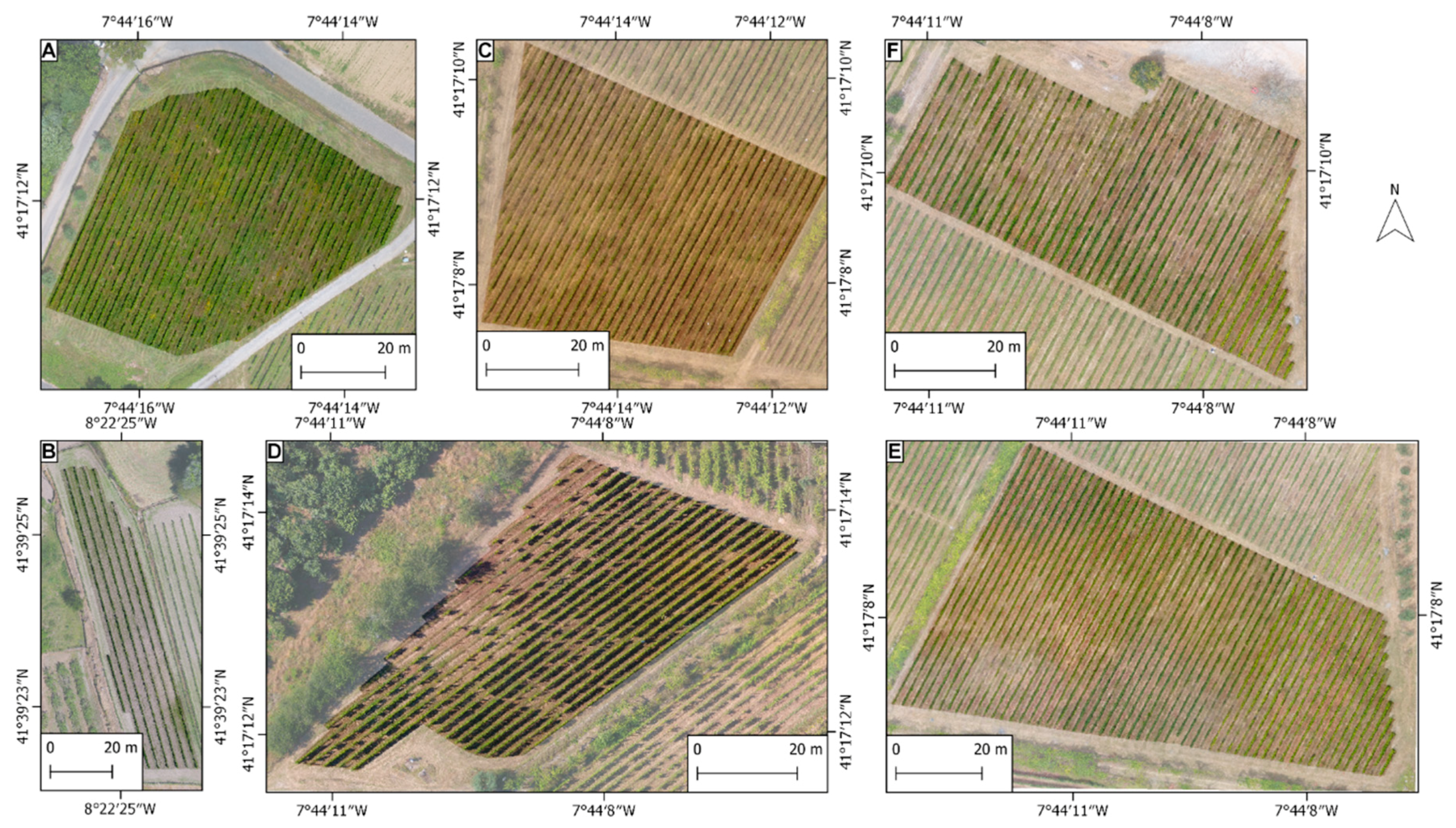
2.1. Data Acquisition

2.1.1. Validation Dataset

A validation dataset, composed of all the surveyed vineyard plots (A to F), was created for accuracy assessment of the individual grapevine detection procedure. Specifically, for the estimation of the number of grapevines and for canopy gaps detection, i.e., parts of vine rows where no grapevine canopy is present (missing plants). For this purpose, only RGB data was considered. The data was collected between May to August 2018 at the following at days of the year (DOY):136 (vineyard plot B); 186 (vineyard plot A); 197 (vineyard plot D); 215 (vineyard plot C); and 219 (vineyard plots E and F).

2.1.2. Multi-Temporal Dataset

Vineyard plots A and B were used for multi-temporal analysis and were surveyed using different UAV-based sensors, namely, RGB, MSP and TIR. The context of these vineyard plots is different: vineyard plot A, located at UTAD campus, is mainly used for experimental purposes, while plot B is a commercial vineyard. Vineyard plot B was selected to be surveyed throughout the vegetative growth cycle. It is composed of seven rows of two white grapevine varieties, four rows of cv. Alvarinho and three rows of cv. Loureiro. Vineyard plot A had a higher incidence of missing grapevines and suffered from powdery and downy mildew due to the conjugation of high air temperature and high humidity levels. These fungi affect the grapevines yield and leaves causing potential losses [56]. It is composed of a collection of recommended Portuguese grapevine varieties.

In the case of vineyard plot A, flight campaigns were conducted in the first and fourth weeks of July and in the third week of August and September (2018), with an average time distance of approximately 26 days in between flight campaigns, covering most parts of the fruit set and veraison phenological stages. As for vineyard B, the flight period is broader encompassing most parts of the grapevine’s phenological development, from the third week of May 2018 until the second week of October 2018, after grape harvesting. The remaining campaigns were performed on the third week of June and July, and on the second week of August 2018. The temporal mean distance between campaigns is 37 days.

For an accurate multi-temporal analysis, six ground control points (GCP) were acquired in different points from the surroundings of each analysed vineyard plot using a GNSS receiver in RTK mode in the TM06/ETRS89 coordinate system to perform imagery alignment during the photogrammetric processing. In order to ensure GCPs’ recognition in TIR imagery, aluminium foil was used, as in Hartmann et al. [57]. Figure 2 presents an example of the aluminium target appearance thermal and RGB images.

2.2. Data Processing

The data acquired in each flight campaign passed through a pre-processing stage by means of photogrammetric processing for computation of different orthorectified outcomes. After this stage, the data was used as input for individual grapevine estimation and computation of different vineyard-related parameters.

2.2.1. Data Pre-Processing

Pix4Dmapper Pro (Pix4D SA, Lausanne, Switzerland) was used for photogrammetric processing. It supports the imagery from all the sensors used in this study, allowing the generation of 3D point clouds using Structure from Motion (SfM) algorithms and, therefore, different orthorectified outcomes. However, depending on the source data, different outcomes were computed. This way, when processing RGB imagery, orthophoto mosaics, DSMs and DTMs were generated. Moreover, crop surface models (CSM) were computed subtracting the DTM altitude values from the DSM. The G% index [58] was computed according to [48], from the RGB orthophoto mosaic, as in (1), by normalizing the green band with the sum of all bands. The data from other sensors used in this study can also generate CSM, but they suffer from smoothing effects since they have less spatial resolution and, therefore, lack of detail [39].

$$\mathrm{G}\%=\mathrm{Green}/\left(\mathrm{Red}+\mathrm{Green}+\mathrm{Blue}\right)$$

(1)

The NDVI was computed using multispectral imagery. Using TIR imagery, the land surface temperature (LST) was computed. However, since crop temperature varies along the day and epoch of the year, it can penalize the multi-temporal data analysis representativeness [28]. Thus, to ensure the most representative results from TIR data, LST from each flight campaign was used to compute the CWSI [25]. This index relies on the usage of upper and lower temperature bounds (T_wet and T_dry) which, respectively, correspond to the temperatures of a well-watered leaf and a non-transpiring leaf. Since GSDs from different sensors were also different, to enable data integration, it was necessary to standardize the GSD. This operation was directly performed in the photogrammetric software, using the gaussian average, being the data resampled to 5 cm GSD. Obviously, this procedure did not improve the resolution of the thermal data, as in practice the original pixel was split divided allowing a direct comparison. This ensures the resolution of the remaining information is maintained and, at the same time, making the image processing stage quicker, and preserving all relevant information. CSM and G% were computed using QGIS software, an open source geographical information system (GIS).

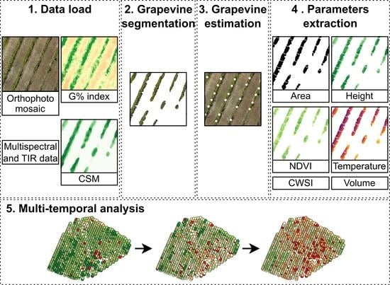
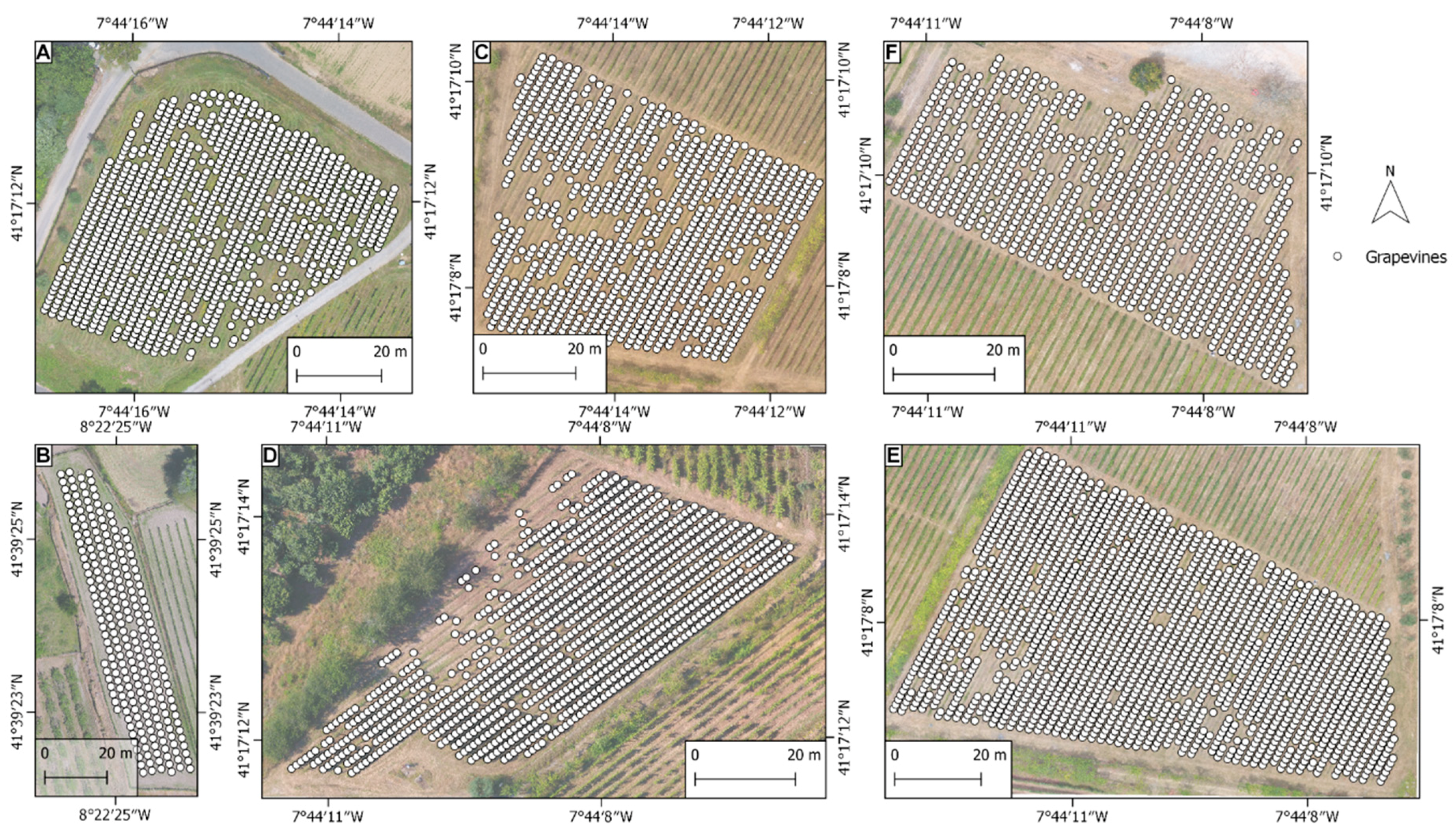
2.2.2. Vine Rows Estimation and Individual Grapevine Estimation

The detection of vineyard vegetation and vine rows was accomplished using the method from Pádua et al. [48]. Figure 3 presents the main stages of the method for individual grapevine estimation and parameters extraction.

Vegetation detection relies on the combination of CSM and G% with image processing techniques for a given vineyard plot P. Both CSM and G% are binarized by thresholding, automatically using the Otsu’s method [59] for G%, and using a height range for the CSM. The resulting images are combined resorting in a new binary image V representing the estimated vineyard vegetation, forming a different group of pixels (clusters). Then, the detected clusters are dilated according to their orientation resulting in the vine rows estimations. By eroding this image, a new image S with the rows central lines is obtained. Considering the equidistance space d between grapevines’ trunks along with S, grapevine plants can be estimated. This is the common scenario in modern vineyards where grapevines are mechanically implanted [53]. This way, points are positioned along the vine rows and then dilated with a morphological line structuring element with the same orientation as the vine rows. Depending on the vineyard training system, the trunk’s position can vary, being in the middle or in edges of the grapevine area. Taking this into account, the grapevines are correctly positioned. The resulting binary image is subjected to a thickening morphological operation, by adding pixels to the border of the clusters but maintaining the clusters as unconnected. The binary image G forms the area where vegetation from each grapevine is confined since they are trained with wires to grow vertically and horizontally in between rows.

2.2.3. Parameters Extraction

By estimating the area of where each grapevine is present within a given plot, it is possible to individually estimate different parameters from biological and physical characteristics. This way, the outcomes from different sensors can be useful to provide grapevine parameters.

This procedure uses the estimated grapevine vegetation V along with G, both are combined as in (2). The result of this combination in a new image E, representing the vegetation for each estimated grapevine, enabling the extraction of biophysical and geometric grapevine parameters from the UAV-based photogrammetric outcomes.

$$e_{i,j}=\{\begin{array}{c}1,\mathrm{if}{v}_{i,j}=1\wedge g_{i,j}=1\\ \mathrm{NaN}, \mathrm{otherwise}\end{array}$$

(2)

Depending on the available data, different parameters can be extracted for each grapevine, namely:

• the area of each grapevine, which is computed by the number of pixels present in each cluster from E multiplied by its squared GSD value;
• the grapevine height, these values are extracted from the CSM, only retrieved in the pixels of E (the remaining CSM pixels are not considered), mean, maximum and minimum values are estimated;
• the volume of the grapevine, it is estimated using both height and area, the different height estimates (mean, maximum and minimum estimated height values) are used to calculate different volume values;
• features are driven from multispectral and TIR imagery, in the case of this study, NDVI, LST and CWSI are masked according to E and its mean, maximum and minimum values are estimated;

Mean value refers to mean value of a given cluster, maximum and minimum values are estimated from the mean value of the higher/lower 10% values, this way, potential outlier pixels are discarded independently from the area of the clusters. Since CWSI needs upper and lower bound temperature values, this was achieved by using the mean temperature values retrieved from LST, considering the mean temperature value of the 10% lowest and highest temperature values to compute T_dry and T_wet, respectively. The estimation of other vegetation indices from different sensors is also supported. In the scope of this study, only NDVI and CWSI are estimated. Still, other parts of the electromagnetic spectrum can also be used. The grapevine mask clusters are associated with the extracted grapevine parameters, which, in turn, are converted to a point shapefile or in a table format. Statistical parameters as the standard deviation of the estimated values are also calculated, but such values are not in the scope of this study.

2.2.4. Multi-Temporal Analysis

The estimated grapevine positions enable its multi-temporal analysis which is crucial to track the grapevine vegetative development over time. This way, the analysis is performed by considering the position of each detected grapevine in a given flight campaign, aiming to individually monitor them regarding the various estimated parameters extracted from the multi-sensor data. This analysis is also performed at the vineyard plot scale, as proposed in Pádua et al. [37].

The multi-temporal analysis is performed by using the detected grapevine estimation in each flight campaign. Using the mask created in G in the first flight campaign upon the estimated grapevine vegetation V from a flight campaign k, it is possible to estimate the different parameters from the available UAV-based data for n flight campaigns. Thus, data from flight campaign k can be used to evaluate the current vineyard status, by statistically assessing the distribution of the different extracted parameters, and to compare it with other flight campaigns. This enables the observation of the grapevines vegetative evolution through the extracted biophysical and geometrical parameters.

2.3. Grapevine Counting Accuracy

For accuracy purposes, the number of estimated grapevines was evaluated. This process was conducted by counting the plants in the vineyard plots, in each vine row, and then different cases were evaluated:

• the total number of estimated grapevines, this value helps to understand the robustness of the method, by considering the total number of grapevines for an analysed vineyard plot;
• the number of existing plants, by cross-referring the actual number of plants observed in-field with the ones estimated from the method; and
• the number of missing grapevines, i.e., grapevines that were missing causing a canopy gap in the vine row.

These values are compared at the vineyard plot level and at the row level.

Grapevine detection was evaluated based on true and false positives (TP/FP) which refer to the number of correct/incorrect estimated grapevines as real grapevines and, similarly, true and false negatives (TN/FN) for non-grapevines. For this purpose, different parameters were evaluated (equation presented in

Table 2. Evaluation parameters in grapevine vegetation classification.

Parameter	Equation
Precision	$Precision=\frac{TP}{TP+FP}$
Recall	$Sensitivity=\frac{TP}{TP+FN}$
False Negative Rate	$FNR=1-\frac{TP}{TP+FN}$
F1score	$F_{1}score=2\left(\frac{Precision\times Recall}{Precision+Recall}\right)$
Overall accuracy	$Accuracy=\frac{TP+TN}{TP+TN+FP+FN}$

), namely:

• precision, the fraction of estimated grapevines that are correctly estimated (TP) rather than wrongly estimated (FP);
• recall, the fraction of grapevines that are correctly detected rather than wrongly estimated;
• false negative rate (FNR), percentage of grapevines falsely classified as being missing;
• F₁score, the harmonic mean of precision and recall measures; and
• overall accuracy, considering all correctly estimated grapevines and missing grapevines in all data.

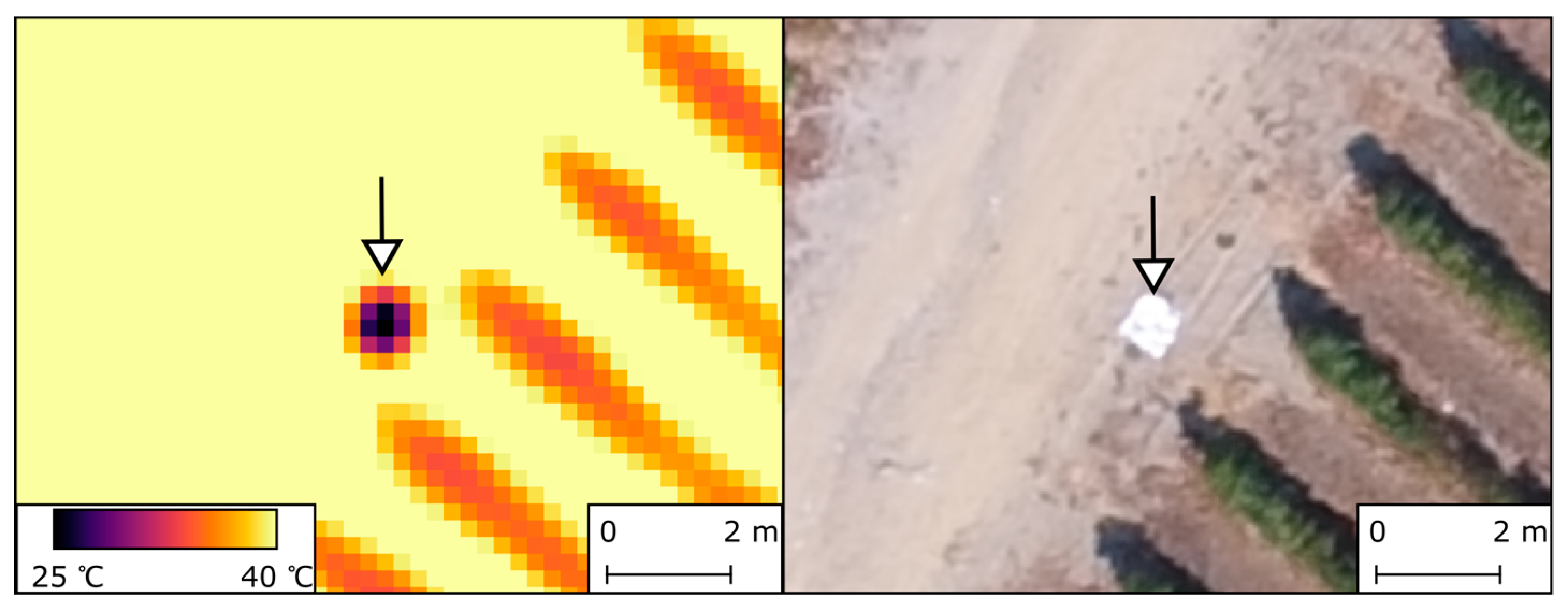
2.4. Data Alignment

Data alignment is crucial in multi-temporal analysis to accurately extract individual grapevine parameters with minor alignment errors. Thus, the photogrammetric processing of the UAV-based imagery from the different sensors was evaluated for each vineyard plot in the flight campaigns encompassed in the multi-temporal dataset. The mean error and root mean square error (RMSE) were used. The RMSE equation is shown in (3), where e_i is the error of each point in a given direction (X, Y, Z) and n the total number of GCPs. This evaluation can further provide the deviation of the acquired UAV-based imagery taken from each sensor along the flight campaigns.

$$\mathrm{RMSE}=\sqrt{\frac{{\sum }_{i=1}^n{e}_i{}^2}{n}}$$

(3)

3. Results

3.1. Grapevine Counting Accuracy

Individual grapevine estimation for different plots of the study area is presented in

Table 3. Number of estimated grapevines when compared to ground truth data observed in-field.

Vineyard Plot	Number of Grapevines		Percentage (%)
	Observed	Estimated
A	1436	1436	100.00
B	234	234	100.00
C	1369	1367	99.85
D	1238	1238	100.00
E	2279	2272	99.69
F	1230	1230	100.00
Total	7786	7777	99.88

. A perfect agreement was observed in vineyards A, B, D, and F, where the number of estimated grapevines per row matched with the ground-truth values. However, for vineyards C and E, the number of estimated vine rows differed by one in each vineyard plot, which was expected since in these vine rows there were no grapevines, thus, these missing grapevines were discarded from further validation. The number of estimated grapevine plants differed by two for vineyard C and seven for vineyard E. Discarding the plants belonging to the undetected vine rows, the overall agreement was 99.88%, missing solely by nine plants (total: 7786, estimated: 7777).

Figure 4 presents the estimated grapevines in each vineyard plot, along with the corresponding numerical assessment shown in

Table 4. Evaluation of the proposed method in the grapevine’s classification for the following parameters: precision, recall, F1score, false negative rate (FNR) and overall accuracy (OA).

Vineyard plot	Precision (%)	Recall (%)	F1score (%)	FNR (%)	OA (%)
A	99.22	98.71	98.96	1.29	98.33
B	100.00	100.00	100.00	0.00	100.00
C	100.00	93.98	96.90	6.02	95.17
D	99.90	96.62	98.23	3.38	97.09
E	99.71	97.67	98.68	2.33	97.58
F	99.00	97.07	98.03	2.93	96.75
Mean	99.64	97.34	98.47	2.66	97.49

. The precision rate was above 99% (mean value of 99.59%), reaching 100% in vineyard B. Regarding recall, also quantifying FN; a mean value of 98.06% was obtained, being the lowest recall value obtained in vineyard C (93.98%). These cases reflect the number of grapevines that were incorrectly classified as missing grapevines (FN). Consequently, FNR was approximately 3% (vineyards C, D and F), while the mean FNR reached 1.94%. In what concerns the harmonic mean of precision and recall metrics (F1score), its mean value is above 98%. The lower value for this metric was observed for vineyard plot F (96.75%), in opposition to vineyards A and B (99%), which had better ranks. For the remaining plots, F1score was within the range of 97–98%. Focusing on accuracy metrics, an overall value of 98% was obtained, with minimum occurrences above 96%. These results seem to represent a good overall agreement concerning individual grapevine classification.

3.2. Multi-Temporal Vineyard Monitoring

Since the used methods anticipated a multi-temporal context application supported through different photogrammetric outcomes from which individual grapevine parameters can be extracted, an analysis using UAV-based RGB, multispectral, and TIR imagery was conducted in vineyards A and B. Moreover, for this type of application, it is important to ensure a reliable imagery alignment, which was also evaluated.

3.2.1. Data Alignment

The spatial accuracy of each orthorectified outcomes, generated from the photogrammetric processing, were evaluated in their mean spatial deviations (X, Y, Z) and mean RMSE. In this case, the UAV-based imagery acquired from RGB, multispectral and TIR sensors, with different spatial resolutions, were used along with georeferenced GCPs. The projection errors obtained in vineyards A and B for each sensor are presented in

Table 5. Mean error, root mean square error (RMSE) and projection errors for the alignment of each project during photogrammetric processing in both analysed vineyard plots, at each flight campaign (F#).

Vineyard Plot	Sensor	F#	Mean (cm)	RMSE (cm)	Projection Error (Pixel)
A	RGB	F1	−0.19	3.15	1.30
		F2	−0.19	4.55	1.21
		F3	0.08	3.65	0.57
		F4	0.06	3.09	0.58
	MSP	F1	0.78	5.47	0.71
		F2	−0.40	5.90	0.43
		F3	0.41	8.22	1.25
		F4	0.24	9.82	0.51
	TIR	F1	0.72	12.39	0.65
		F2	−0.98	13.34	0.54
		F3	3.82	19.38	0.74
		F4	4.70	16.87	0.90
B	RGB	F1	−0.37	3.68	1.30
		F2	0.02	2.20	0.63
		F3	0.00	1.73	0.57
		F4	−0.03	1.81	0.57
		F5	−0.01	1.76	0.58
	MSP	F1	−0.63	4.66	0.50
		F2	0.24	4.38	0.85
		F3	−1.16	3.84	0.93
		F4	−0.76	4.99	0.53
		F5	0.11	6.35	0.75
	TIR	F1	2.84	11.30	0.47
		F2	3.14	16.52	0.76
		F3	2.35	15.55	0.66
		F4	2.60	14.02	0.59
		F5	1.55	14.30	0.77

, for each flight campaign. Overall, the errors are lower for RGB, below 5 cm; followed by multispectral imagery, with errors ranging from 5 cm to 10 cm; and when processing TIR imagery, higher error rates were obtained ranging from 10 cm to 20 cm. Pixel projection error was similar in all sensors, i.e., from approximately 0.5 to 1 pixel, being generally higher for RGB imagery. The overall mean RMSE values in vineyard A were 3.61 cm for the RGB imagery, 7.35 cm for the multispectral imagery, and 15.50 cm for the TIR imagery, while in vineyard B they were, respectively, 2.24 cm, 4.84 cm, and 14.34 cm. The mean pixel projection error of all campaigns was lower than one pixel in all sensors; it was higher in the RGB, followed by the multispectral and TIR imagery.

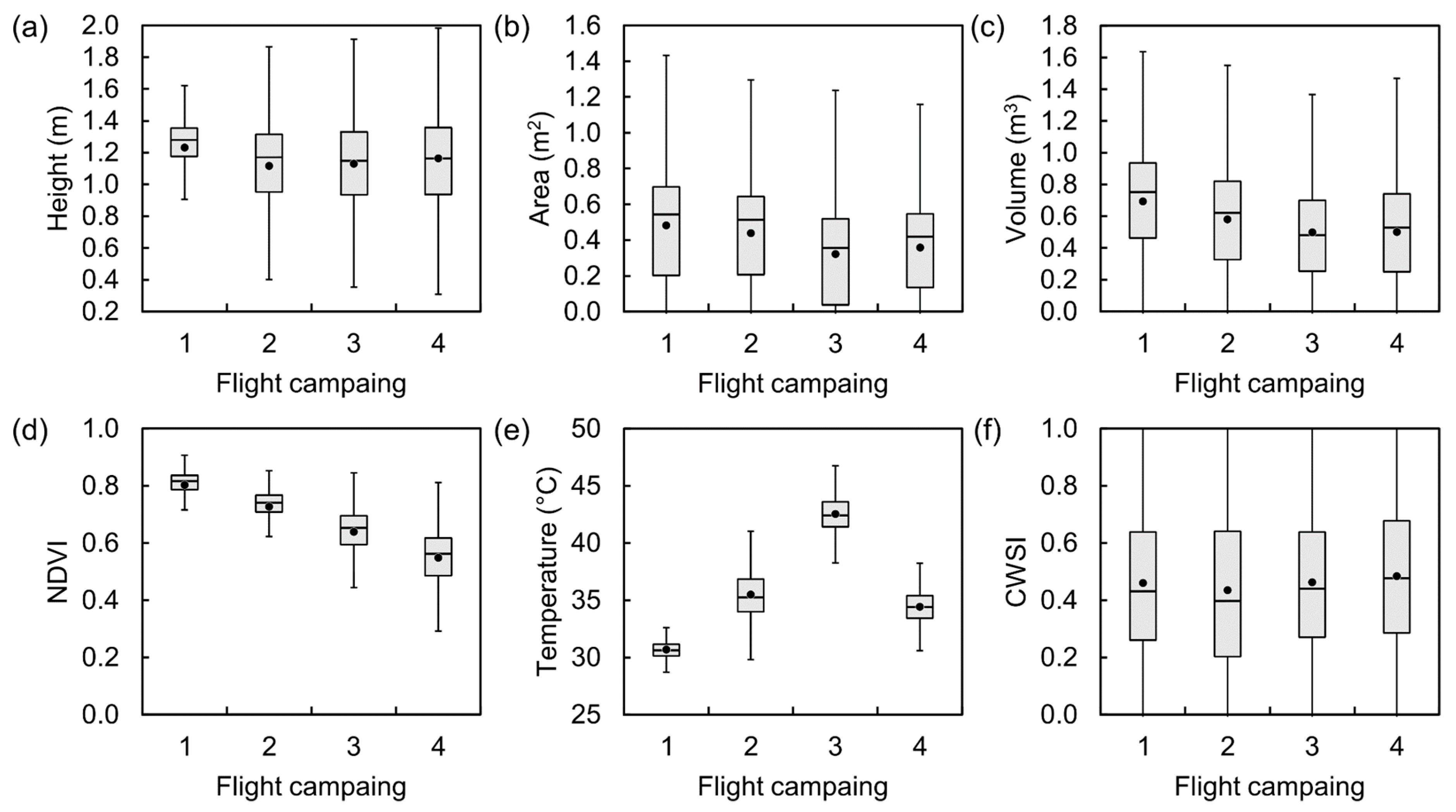
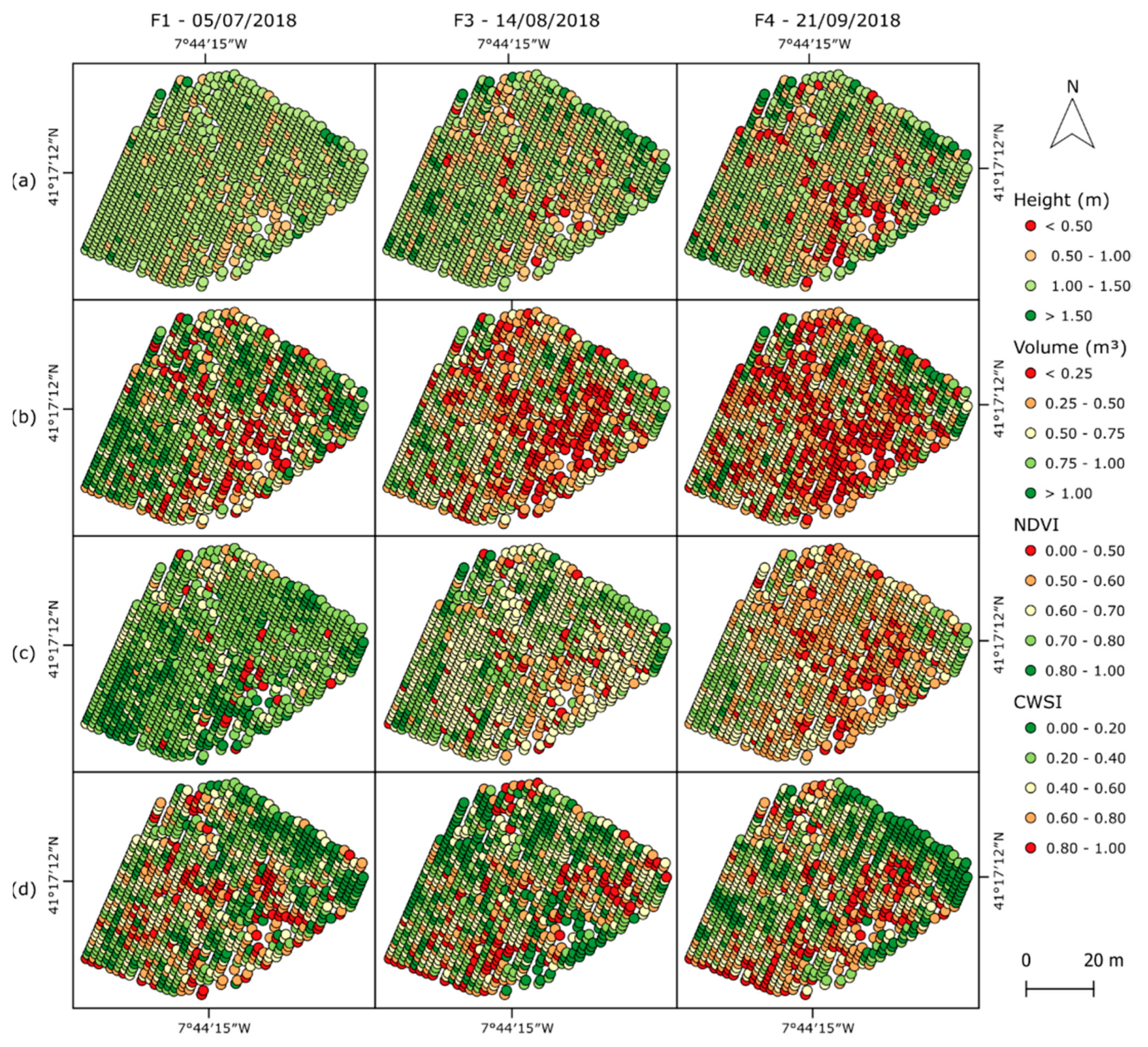
3.2.2. Vineyard Plot A

The applied method enables the estimation of vegetation (grapevine and. inter-row vegetation) present in the vineyard plot. In between the flight campaigns, an increment of grapevine vegetation area was observed from the first to the second flight campaign (from 675 m² to 782 m², corresponding to a 16% increase). From the second to the third flight campaign, there was a decline of 35% (−272 m²). For the remaining flight campaigns, the grapevine vegetation area remained unchanged (around 500 m²). The same behaviour was observed in grapevine volume, where 877 m³ was estimated in the first flight campaign, 939 m³ (growth of 7%) for the second flight campaign, followed by 619 m³ (decline of 34%) and 610 m³ (decline of 1%), for the third and fourth flight campaigns, respectively. Focusing on the inter-row vegetation, its area declined from the first to second flight campaigns (from 1221 m² to 6 m²), and then remained unchanged on subsequent flights (lower than 90 m²).

Figure 5 provides the distribution of the mean values of the different parameters extracted from the estimated grapevine plants. The flight campaigns were carried out with a significant vegetation development from fruit set to harvest. This way, the height distribution in the different flight campaigns (Figure 5a) did not vary significantly, starting with a mean height of 1.23 m in the first flight campaign, and stabilizing around 1.13 m in the remaining campaigns. In what concerns the grapevine area and volume (Figure 5b,c), both parameters presented a similar behaviour, declining from the first to the last flight campaign. The grapevines mean area starts at 0.44 m² in the first campaign and a progressive decrease can be observed until the last campaign, in which the grapevine mean area ends up at 0.32 m². In terms of the mean grapevine canopy volume, it is 0.69 m³ in the first flight campaign, 0.58 m³ in the second one and 0.50 m³ in the remaining flight campaigns. Considering the distribution of the NDVI values (Figure 5d), a decline was verified when comparing the values of the previous campaigns sequence in which 0.80, 0.73, 0.66, and 0.55 of grapevine mean NDVI were respectively reached. Regarding the parameters extracted from the thermal infrared imagery, both grapevine temperature and CWSI (Figure 5e,f) presented distinct distributions. The temperature values were lower in the first flight campaign and higher in the third flight campaign. Despite the mean temperature variability through the flight campaigns, CWSI distribution is similar.

Figure 6 presents the main parameters extracted for the estimated grapevines. The grapevine’s height distribution (Figure 6a) suffered a decline along the flight campaigns. In fact, 87% of estimated heights were higher than 1.0 m in the first flight campaign, falling to 77% in the second flight campaign, 64% in the third and 72% in the fourth flight campaign. Regarding plants with heights lower 0.5 m, no estimates were presented in the first flight campaign, whereas in the following campaigns this number represented 0.3%, 8% and 2%, of the total estimates. Individual grapevine canopy volume (Figure 6b) presented a similar trend. In the first flight campaign, 53% of the grapevines showed a volume greater than 0.75 m³, while in the following flight campaigns only 39%, 24% and 19% were greater than 0.75 m³. Regarding plants with a volume greater than 1 m³, they represented 19%, 10%, 6% and 4% of the estimated grapevines. Considering individual grapevine NDVI values (Figure 6c) bigger than 0.7, a total of 85% higher were identified in the first flight campaign, 60% in the second, 38% in the third, and 16% in fourth flight campaign. Focusing on the CWSI (Figure 6d), 75% of the grapevine plants were lower than 0.6 in the first three flight campaigns, while in the last flight campaign this value is 70%.

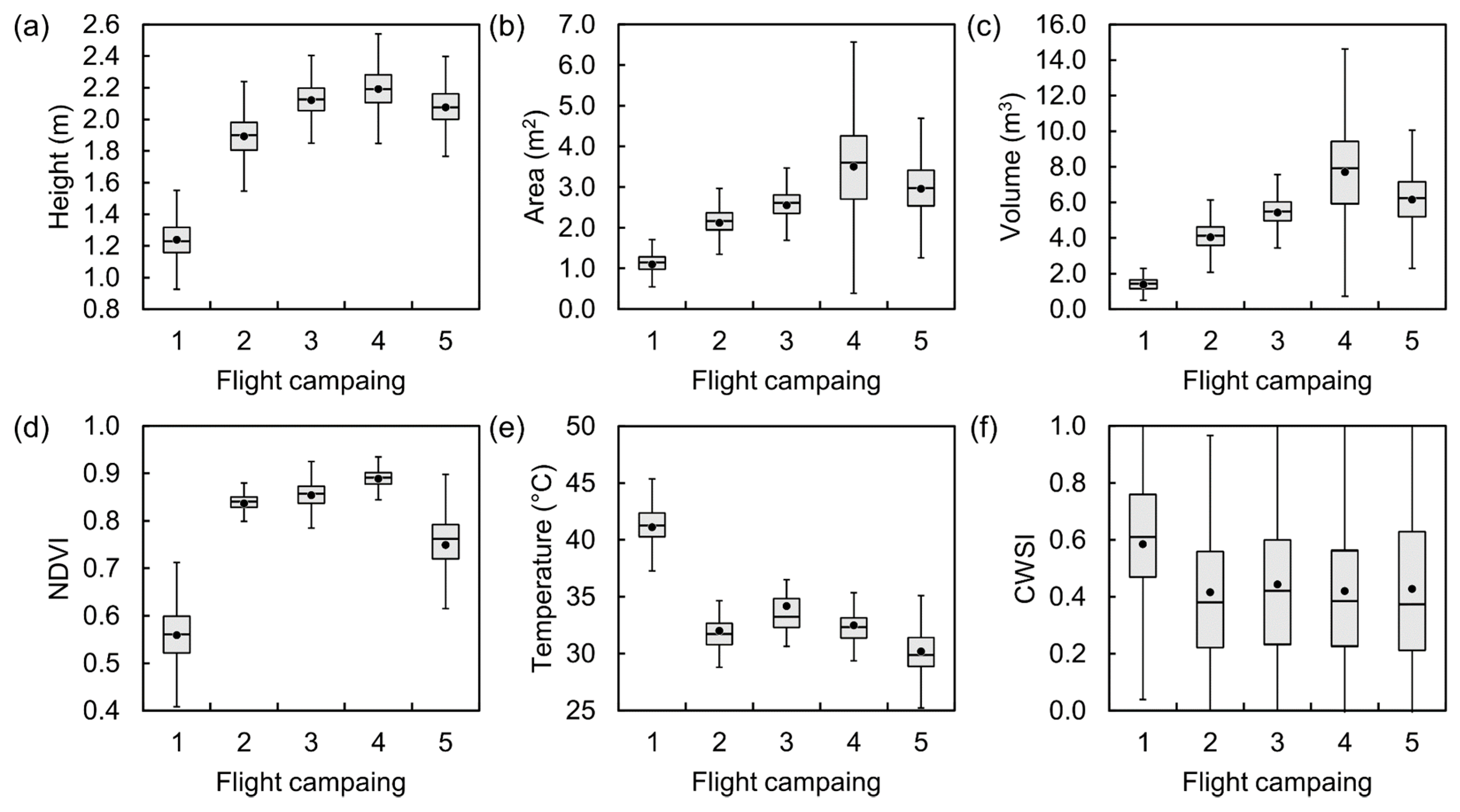
3.2.3. Vineyard Plot B

In what concerns vineyard B, a broader period was analysed (from May to October 2018), encompassing most of the vineyard vegetative development from flowering to harvesting. A growth trend of the grapevine vegetation area and volume is observed across the first four flight campaigns (growth of 218%, from 262 m² to 833 m² and 463%, from 339 m³ to 1301 m³). In the last campaign, a decline of 15% (−128 m²) in area and 21% (−401 m³) in volume was verified. From the second to third flight campaigns, there was a canopy management operation (leaf removal), due to the smaller growth area in between these flights (20% and 101 m²). As for inter-row vegetation, this value increases until July (from 34 m² to 546 m²) and decreases in August (34 m²), with a small growth in October (to 83 m²).

The estimation of the individual grapevines position in the vineyard enabled us to estimate several parameters. Their distribution is presented in Figure 7. Height distribution (Figure 7a) was lower in the first flight campaign with a mean value of 1.24 m, then increased until the fourth flight campaign and declined in the last one. Similar trends were observed in other geometrical parameters such as area and volume (Figure 7b,c), as well as in the NDVI (Figure 7d). Indeed, from the first to the second flight campaigns, a significant growth was registered. The mean grapevine area increased almost to double (from 1.10 m² to 2.12 m²), and the mean grapevine volume increased 193% (from 1.38 m³ to 4.04 m³). In what concerns the grapevines NDVI values, the mean value ranged from 0.56 in the first flight campaign, to 0.84 in the second, 0.86 in the third, 0.89 in the fourth and declined to 0.76 in the last flight. As for LST (Figure 7e) and CWSI (Figure 7f) values, a different trend was observed, the first flight campaign presented a higher temperature than the remaining ones (approximately 10 °C higher), while CWSI values spanned towards higher values in the first flight campaign and lower values in remaining flight campaigns, where most of the data is located below 0.5.

The individual grapevine values estimated for each parameter in the most representative flight campaigns are presented in Figure 8. From the first to the remaining flight campaigns (Figure 8a–c), an overall numerical increase of assessed characteristics can be noted, while a decline from the fourth to fifth flight campaign is better observed in the NDVI, rather than with height or volume. Most of the height values (Figure 8a) in the first flight campaign are below 1.5 m, whereas in the remaining flight campaigns they are higher than 1.5 m. As for grapevine canopy volume (Figure 8b), in the first flight campaign all plants show a value below 4 m³, estimations made upon data from the second flight campaign point out a rate of 57% of grapevine plants greater than 4m³, being above 94% in the remaining flight campaigns. NDVI values (Figure 8c) are lower than 0.7 in the first flight campaign (0.56 mean value) and higher than it in the remaining flight campaigns, excluding the last one where 82% of the grapevines were higher than 0.7. For CWSI, 53% of the grapevines presented a value higher than 0.6 in the first flight campaign, but in the remaining campaigns it is lower, as an example, it represents 21% and 28%, respectively, in the fourth and fifth campaigns.

4. Discussion

4.1. Grapevine Counting Accuracy

The results presented in Section 3.1 document the method’s effectiveness in the individual grapevine estimation using the six vineyard plots analysed. As for the number of grapevines presented in each vineyard plot (Table 3), the method showed 100% accuracy for vineyard plots A, B, D and F. However, for vineyard plots C and E, there was an under-estimation in the number of grapevines in both cases, due to the lack of one plant per vine row. Still, a mean accuracy value of 99.88% was achieved. This is related to the way that the vine rows were estimated, the distance of the rows was smaller than its ground-truth, possibly related to the automatic vine row orientation used during their estimation. Furthermore, as stated in the results section, there were two vine rows that were not detected, one in vineyard plot C (three grapevines) and another in vineyard D (five grapevines). However, since there were no grapevines present in those plots, they were discarded from this evaluation procedure.

As for grapevine identification, the results from the performed evaluation were slightly lower (Table 4), which is related to FP and FN estimations for grapevines. Nevertheless, a mean overall accuracy of 97.5% was achieved. It can be stated that the method tends to overestimate grapevines rather than underestimate since more FN cases were identified (a mean of 2.0% and a mean of 0.4% FP). In vineyard A, the percentage of FP and FN was 1.6% representing, respectively, 8 and 10 cases. The higher number of FP was verified in vineyard F with 10 cases (1%), whereas a higher number of FN was reached in vineyard E with 49 cases (2.4%). However, vineyard F had the highest percentage of FN cases with 3% (30 occurrences). Cases of grapevines classified as missing (FP) can be justified by erroneous three-dimensional reconstruction of the surveyed vineyard plots. Increasing the imagery overlap in the mission plan stage can help to mitigate this issue since more common tie points will be found in correspondent images. The grapevine plants from the commercial vineyard (vineyard plot B) were correctly estimated, as this plot only composed seven vine rows and had only two missing grapevine plants. In Primicerio et al. [53], this issue was addressed by evaluating a total of 211 missing plants (incidence of 9.4%), in which the parameter found with most correlation was the grapevine area. Different area thresholds were considered, based on the cardinality of each cluster attributed to grapevine plants, wherein lower values showed to be more suitable for missing plant discrimination but inducing the FP number growth, while higher values result in the inverse behaviour. In Matese and Di Genaro [54], the results demonstrated 80% accuracy in missing plants detection with the application of their method. Authors stated that FP results (plants estimated as a missing plant) were related to their low vegetative development, while FN results (missing plant classified as a plant) were related to the high presence of weeds and overlap of adjacent plants. However, neither of these studies considered height properties. In De Castro et al. [38] an overall accuracy of 95.3% was obtained in the analysis of three vineyard plots in Northeastern Spain at two different epochs (July and September). Similarly, to this study, according to the authors, most of the misclassification cases were related to grapevines lower vegetative development (thin branches and fewer leaves) which led to issues in the 3D canopy reconstruction through photogrammetric processing. Regarding FN cases, it can be justified by the growth of adjacent grapevines which tends to cover missing spots in the wires, making it difficult to estimate missing plants. This way, as a future direction, machine learning classification should be considered to detect the number of missing grapevines. Moreover, as stated by Matese and Di Genaro [54], by selecting an anticipated period to conduct this type of survey would increase the results accuracy, by having plants with less vegetative development, which would avoid the presence of adjacent grapevine vegetation in missing plant areas.

4.2. Data Alignment

Since one of the main goals of this study is to extract grapevine properties from different outcomes through photogrammetric processing of UAV-based imagery from different sensors, a correct data alignment must be ensured to mitigate data alignment errors. Aiming to reduce geolocation errors from a few metres to some centimetres [60]. In Turner et al. [61] the same tendency was inferred, when compared to the results obtained in this study. More specifically, the overall RMSE values were approximately 1.9 cm for RGB imagery (1 cm GSD), 6.4 cm for multispectral imagery (3 cm GSD), and 17.8 cm for TIR imagery (10 cm GSD). In their study, the authors used a higher number of GCPs along with a lower flight height and almost half of the spatial resolution used in this study. The need of GCPs for multi-sensor data alignment will be mitigated by the technological development of sensors by combining visible, multispectral and TIR data into a single sensor, this is the case of the MicaSense Altum (MicaSense Inc., Washington, United States of America) which provides radiometrically corrected blue, green, red, red edge, NIR spectral bands along with TIR imagery. This way, in a single UAV flight, all data is acquired and photogrammetric processing can be achieved in a single project.

4.3. Multi-Temporal Vineyard Monitoring

By analysing the results obtained through the method application in both vineyards A and B (Section 3.2.2 and Section 3.2.3), the spatial grapevine variability is noticeable. Furthermore, the multi-temporal analysis enabled us to track the changes throughout the analysed periods.

In what concerns the experimental vineyard (vineyard A), it presented a higher incidence of missing grapevines, which is associated with the occurrence of phytosanitary problems and to the presence of different grapevine varieties, wherein a higher data variability is clearly visible (Figure 6). Areas with a better grapevine overall status, are located in the upper right and bottom left parts of the vineyard. Higher NDVI values and grapevine volume were detected in those areas throughout the flight campaigns, as this is more notorious in all flight campaigns for the estimated grapevine volume and in the first three flight campaigns for NDVI. With respect to CWSI, only the first and last two flight campaigns highlighted this behaviour. On the other hand, the southern central part showed the lowest results. The grapevines in this region presented a lower volume, particularly in the last two flight campaigns, along with higher CWSI values (potential water stress) and lower NDVI values.

The commercial vineyard plot (vineyard B) presented a high vegetative dynamic over the analysed period, its parameters grew throughout the flight campaigns and declined after the harvest season (Figure 7). Its geometrical features (height, area, and volume) along with NDVI showed a higher development from the first to second flight campaigns. These results are related to both phenological stages and training systems implemented in the Vinho Verde wine region. This vineyard presented overall good results as confirmed by the estimated grapevine values in the flight campaigns (Figure 8). The northern part presented a higher grapevine volume when analysing each flight campaign, while for NDVI this was only verified in the last two campaigns. The southern part presented some water stress signs (Figure 8d) in the last two flight campaigns, along with lower grapevine volume verified on all flight campaigns, and lower NDVI values were only observed in the last flight campaign. Regarding CWSI, the inferior grapevine vegetative development verified in the first flight campaign led to the estimation of potential water stress in the upper part of the vineyard, while in the last flight campaign the higher CWSI agreed with the lower NDVI values.

When comparing the commercial (vineyard B) and the experimental (vineyard A) vineyard, the former obtained better results in almost all parameters. A higher spatial heterogeneity was verified in vineyard A, while vineyard B presented a more homogeneous development, as can be seen when analysing the grapevine canopy volume and NDVI. However, some similar trends were detected in both vineyards, an overall decline of the NDVI values in the last flight campaigns and an agreement between NDVI with the estimated grapevine volume and with the CWSI values was observed. The decline of NDVI in the last flight campaigns can be related to the leaf senescence and, consequently, its discolouration [62,63]. The relationships among the NDVI and volume relationships were verified in other studies [24] that showed that both of these parameters are related with LAI, which in fact, is also verified in this study.

Grapevines located in the southern parts (first plant of the rows) of the analysed vineyards presented potential water stress in the CWSI, an observation that gains meaning in the last two flight campaigns of vineyard B and in the first, third and fourth flight campaigns in vineyard A. This can be considered as outliers, since higher temperatures are observed due to heat advection from the soil in proximity to the edges of the rows of the grapevine canopy, which can affect, in a significant manner, the air temperature, with an increase in the loss of water by evapotranspiration [64]. These results corroborated with Tucci et al. [65] where external rows in a terraced vineyard presented higher temperatures due to solar exposition and shadowing effects when compared with internal vine rows. Although the individual grapevine temperature is estimated, this parameter showed to be ineffective to be evaluated in a multitemporal analysis. It is useful to understand the global temperature context on the flight campaign day. The CWSI trends shown a more stabilized distribution since this index represents a normalization throughout the flight campaigns. Moreover, other TIR-based indices can be computed, as it is the case of stomatal conductance indices Ig and I3 [66], which, respectively, implicated increases with stomatal conductance and correlates it with stomatal resistance. The same applies to other multispectral-based vegetation indices and to hyperspectral data, as long as it comes in an orthorectified format. Usually, published studies resort to NDVI to produce vigour maps and use that information to improve the decision support at the vineyard plot scale [13,23,67]. The approach proposed in this study provides a more incisive analysis. Multi-sensor parameters are extracted at the plant level and are not exclusively relying on qualitative analysis.

5. Conclusions

This study explores the usage of UAV-based photogrammetric outcomes to extract individual grapevine geometrical and biophysical parameters within vineyard plots. Missing plants and other vegetation are detected but not considered to perform multi-temporal analysis over a series of flight campaigns. Three different types of sensors (RGB, multispectral and TIR) were used. By estimating vine rows and the individual position of each plant, several parameters can be extracted at the plot level, namely the: number of vine rows; number of plants; and number of missing plants and grapevine vegetation area; and at the plant level, the: position; length; width; area; volume; vigour (driven from NDVI); temperature from (TIR) and water status (driven from CWSI). The two multi-temporal analyses conducted in the two different vineyards presented in this study confirmed the method’s suitability for plant-specific analysis, allowing us to assess the different estimated parameters and to establish relationships among them and between flight campaigns. This way, the methods employed in this study enable an overview of the current status of the grapevine plants and the monitoring of their evolution over time. The estimated geometrical and biophysical parameters can significantly help farmers and/or winemakers understand the current vineyard overall status and can be used as a decision support tool to apply treatments in certain plants and to observe their response with multi-temporal analysis, helping to improve grapevines health. Moreover, it can be used to compare growth seasons from different years by extending the flight campaigns.

The potential of the method can be extended for different applications, it can help in the decision support by means of grapevine growth and status evaluation, and the individual grapevine water status estimation. Moreover, the different extracted parameters can be used to create datasets for supervised and unsupervised classification methods for disease detection and to improve the results in the detection of missing grapevines. The extracted individual grapevine parameters can be used for computation of prescription maps for individual grapevine treatment in PV plant-specific applications and to estimate individual grapevine production. The topographical data produced from the photogrammetric processing along with the position of each grapevine and its estimated parameters can be used to reproduce a 3D virtual vineyard environment. As such, this information can be used in augmented reality applications for easier vineyard in-field inspections.

References

1. Proffitt, A.P.B.; Bramley, R.; Lamb, D.; Winter, E. Precision Viticulture: A New Era in Vineyard Management and Wine Production; Winetitles: Ashford, Australia, 2006; ISBN 978-0-9756850-4-4. [Google Scholar]
2. Zarco-Tejada, P.J.; Hubbard, N.; Loudjani, P. Precision Agriculture: An Opportunity for EU Farmers-Potential Support with the CAP 2014–2020; Joint Research Centre (JRC) of the European Commission Monitoring Agriculture ResourceS (MARS): Brussels, Belgium, 2014. [Google Scholar]
3. Matese, A.; Di Gennaro, S.F. Technology in precision viticulture: A state of the art review. Int. J. Wine Res. 2015, 7, 69–81. [Google Scholar] [CrossRef] [Green Version]
4. Zhang, C.; Kovacs, J.M. The Application of Small Unmanned Aerial Systems for Precision Agriculture: A Review. Precis. Agric. 2012, 13, 693–712. [Google Scholar] [CrossRef]
5. Steyn, J.; Tudó, J.L.A.; Benavent, J.L.A. Grapevine vigour and within vineyard variability: A review. Int. J. Sci. Eng. Res. 2016, 7, 1056–1065. [Google Scholar]
6. Karakizi, C.; Oikonomou, M.; Karantzalos, K. Spectral Discrimination and Reflectance Properties of Various Vine Varieties from Satellite, UAV and Proximate Sensors. Int. Arch. Photogramm. Remote Sens. Spat. Inf. Sci. 2015, 40, 31. [Google Scholar] [CrossRef] [Green Version]
7. Tisseyre, B.; Ojeda, H.; Taylor, J. New technologies and methodologies for site-specific viticulture. J. Int. Des. Sci. De La Vigne Et Du Vin 2007, 41, 63–76. [Google Scholar] [CrossRef]
8. Martín, P.; Zarco-Tejada, P.; González, M.; Berjón, A. Using hyperspectral remote sensing to map grape quality inTempranillo’vineyards affected by iron deficiency chlorosis. Vitis-Geilweilerhof 2007, 46, 7. [Google Scholar]
9. Hall, A.; Lamb, D.W.; Holzapfel, B.; Louis, J. Optical remote sensing applications in viticulture-a review. Aust. J. Grape Wine Res. 2002, 8, 36–47. [Google Scholar] [CrossRef]
10. Johnson, L.; Roczen, D.; Youkhana, S.; Nemani, R.; Bosch, D. Mapping vineyard leaf area with multispectral satellite imagery. Comput. Electron. Agric. 2003, 38, 33–44. [Google Scholar] [CrossRef]
11. Johnson, L.F.; Roczen, D.; Youkhana, S. Vineyard canopy density mapping with IKONOS satellite imagery. In Proceedings of the Third International Conference on Geospatial Informationin Agriculture and Forestry, Denver, CO, USA, 5–7 November 2001. [Google Scholar]
12. Matese, A.; Primicerio, J.; Di Gennaro, F.; Fiorillo, E.; Vaccari, F.P.; Genesio, L. Development and Application of an Autonomous and Flexible Unmanned Aerial Vehicle for Precision Viticulture. Acta Hortic. 2012, 978, 63–69. [Google Scholar] [CrossRef]
13. Khaliq, A.; Comba, L.; Biglia, A.; Ricauda Aimonino, D.; Chiaberge, M.; Gay, P. Comparison of Satellite and UAV-Based Multispectral Imagery for Vineyard Variability Assessment. Remote Sens. 2019, 11, 436. [Google Scholar] [CrossRef] [Green Version]
14. Mendes, J.; Dos Santos, F.N.; Ferraz, N.; Couto, P.; Morais, R. Vine Trunk Detector for a Reliable Robot Localization System. In Proceedings of the 2016 International Conference on Autonomous Robot Systems and Competitions (ICARSC), Braganca, Portugal, 4–6 May 2016; pp. 1–6. [Google Scholar]
15. Milella, A.; Marani, R.; Petitti, A.; Reina, G. In-field high throughput grapevine phenotyping with a consumer-grade depth camera. Comput. Electron. Agric. 2019, 156, 293–306. [Google Scholar] [CrossRef]
16. Rosell, J.R.; Llorens, J.; Sanz, R.; Arnó, J.; Ribes-Dasi, M.; Masip, J.; Escolà, A.; Camp, F.; Solanelles, F.; Gràcia, F.; et al. Obtaining the three-dimensional structure of tree orchards from remote 2D terrestrial LIDAR scanning. Agric. For. Meteorol. 2009, 149, 1505–1515. [Google Scholar] [CrossRef] [Green Version]
17. Morais, R.; Fernandes, M.A.; Matos, S.G.; Serôdio, C.; Ferreira, P.J.S.G.; Reis, M.J.C.S. A ZigBee multi-powered wireless acquisition device for remote sensing applications in precision viticulture. Comput. Electron. Agric. 2008, 62, 94–106. [Google Scholar] [CrossRef]
18. Matese, A.; Toscano, P.; Di Gennaro, S.F.; Genesio, L.; Vaccari, F.P.; Primicerio, J.; Belli, C.; Zaldei, A.; Bianconi, R.; Gioli, B. Intercomparison of UAV, Aircraft and Satellite Remote Sensing Platforms for Precision Viticulture. Remote Sens. 2015, 7, 2971–2990. [Google Scholar] [CrossRef] [Green Version]
19. Pádua, L.; Vanko, J.; Hruška, J.; Adão, T.; Sousa, J.J.; Peres, E.; Morais, R. UAS, sensors, and data processing in agroforestry: A review towards practical applications. Int. J. Remote Sens. 2017, 38, 2349–2391. [Google Scholar] [CrossRef]
20. Colomina, I.; Molina, P. Unmanned aerial systems for photogrammetry and remote sensing: A review. Isprs J. Photogramm. Remote Sens. 2014, 92, 79–97. [Google Scholar] [CrossRef] [Green Version]
21. Rouse, J.W., Jr.; Haas, R.H.; Schell, J.A.; Deering, D.W. Monitoring Vegetation Systems in the Great Plains with Erts. Nasa Spec. Publ. 1974, 351, 309. [Google Scholar]
22. Caruso, G.; Tozzini, L.; Rallo, G.; Primicerio, J.; Moriondo, M.; Palai, G.; Gucci, R. Estimating biophysical and geometrical parameters of grapevine canopies (‘Sangiovese’) by an unmanned aerial vehicle (UAV) and VIS-NIR cameras. VITIS J. Grapevine Res. 2017, 56, 63–70. [Google Scholar]
23. Campos, J.; Llop, J.; Gallart, M.; García-Ruiz, F.; Gras, A.; Salcedo, R.; Gil, E. Development of canopy vigour maps using UAV for site-specific management during vineyard spraying process. Precis. Agric. 2019, 20, 1136–1156. [Google Scholar] [CrossRef] [Green Version]
24. Matese, A.; Di Gennaro, S.F.; Santesteban, L.G. Methods to compare the spatial variability of UAV-based spectral and geometric information with ground autocorrelated data. A case of study for precision viticulture. Comput. Electron. Agric. 2019, 162, 931–940. [Google Scholar] [CrossRef]
25. Idso, S.B.; Jackson, R.D.; Pinter, P.J.; Reginato, R.J.; Hatfield, J.L. Normalizing the stress-degree-day parameter for environmental variability. Agric. Meteorol. 1981, 24, 45–55. [Google Scholar] [CrossRef]
26. Santesteban, L.G.; Di Gennaro, S.F.; Herrero-Langreo, A.; Miranda, C.; Royo, J.B.; Matese, A. High-resolution UAV-based thermal imaging to estimate the instantaneous and seasonal variability of plant water status within a vineyard. Agric. Water Manag. 2017, 183, 49–59. [Google Scholar] [CrossRef]
27. Baluja, J.; Diago, M.P.; Balda, P.; Zorer, R.; Meggio, F.; Morales, F.; Tardaguila, J. Assessment of vineyard water status variability by thermal and multispectral imagery using an unmanned aerial vehicle (UAV). Irrig. Sci. 2012, 30, 511–522. [Google Scholar] [CrossRef]
28. Bellvert, J.; Zarco-Tejada, P.J.; Girona, J.; Fereres, E. Mapping crop water stress index in a ‘Pinot-noir’ vineyard: Comparing ground measurements with thermal remote sensing imagery from an unmanned aerial vehicle. Precis. Agric. 2013, 15, 361–376. [Google Scholar] [CrossRef]
29. Bellvert, J.; Marsal, J.; Girona, J.; Zarco-Tejada, P.J. Seasonal evolution of crop water stress index in grapevine varieties determined with high-resolution remote sensing thermal imagery. Irrig. Sci. 2015, 33, 81–93. [Google Scholar] [CrossRef]
30. Tilly, N.; Hoffmeister, D.; Cao, Q.; Huang, S.; Lenz-Wiedemann, V.; Miao, Y.; Bareth, G. Multitemporal crop surface models: Accurate plant height measurement and biomass estimation with terrestrial laser scanning in paddy rice. J. Appl. Remote Sens. 2014, 8, 083671. [Google Scholar] [CrossRef]
31. Du, M.; Noguchi, N. Monitoring of Wheat Growth Status and Mapping of Wheat Yield’s within-Field Spatial Variations Using Color Images Acquired from UAV-camera System. Remote Sens. 2017, 9, 289. [Google Scholar] [CrossRef] [Green Version]
32. Li, W.; Niu, Z.; Chen, H.; Li, D.; Wu, M.; Zhao, W. Remote estimation of canopy height and aboveground biomass of maize using high-resolution stereo images from a low-cost unmanned aerial vehicle system. Ecol. Indic. 2016, 67, 637–648. [Google Scholar] [CrossRef]
33. Bendig, J.; Bolten, A.; Bennertz, S.; Broscheit, J.; Eichfuss, S.; Bareth, G. Estimating Biomass of Barley Using Crop Surface Models (CSMs) Derived from UAV-Based RGB Imaging. Remote Sens. 2014, 6, 10395–10412. [Google Scholar] [CrossRef] [Green Version]
34. Díaz-Varela, R.A.; De la Rosa, R.; León, L.; Zarco-Tejada, P.J. High-Resolution Airborne UAV Imagery to Assess Olive Tree Crown Parameters Using 3D Photo Reconstruction: Application in Breeding Trials. Remote Sens. 2015, 7, 4213–4232. [Google Scholar] [CrossRef] [Green Version]
35. Marques, P.; Pádua, L.; Adão, T.; Hruška, J.; Peres, E.; Sousa, A.; Sousa, J.J. UAV-Based Automatic Detection and Monitoring of Chestnut Trees. Remote Sens. 2019, 11, 855. [Google Scholar] [CrossRef] [Green Version]
36. Johansen, K.; Raharjo, T.; McCabe, M.F. Using Multi-Spectral UAV Imagery to Extract Tree Crop Structural Properties and Assess Pruning Effects. Remote Sens. 2018, 10, 854. [Google Scholar] [CrossRef] [Green Version]
37. Pádua, L.; Marques, P.; Hruška, J.; Adão, T.; Peres, E.; Morais, R.; Sousa, J.J. Multi-Temporal Vineyard Monitoring through UAV-Based RGB Imagery. Remote Sens. 2018, 10, 1907. [Google Scholar] [CrossRef] [Green Version]
38. de Castro, A.I.; Jiménez-Brenes, F.M.; Torres-Sánchez, J.; Peña, J.M.; Borra-Serrano, I.; López-Granados, F. 3-D Characterization of Vineyards Using a Novel UAV Imagery-Based OBIA Procedure for Precision Viticulture Applications. Remote Sens. 2018, 10, 584. [Google Scholar] [CrossRef] [Green Version]
39. Matese, A.; Di Gennaro, S.F.; Berton, A. Assessment of a canopy height model (CHM) in a vineyard using UAV-based multispectral imaging. Int. J. Remote Sens. 2017, 38, 2150–2160. [Google Scholar] [CrossRef]
40. Pádua, L.; Marques, P.; Adão, T.; Guimarães, N.; Sousa, A.; Peres, E.; Sousa, J.J. Vineyard Variability Analysis through UAV-Based Vigour Maps to Assess Climate Change Impacts. Agronomy 2019, 9, 581. [Google Scholar] [CrossRef] [Green Version]
41. Comba, L.; Gay, P.; Primicerio, J.; Ricauda Aimonino, D. Vineyard detection from unmanned aerial systems images. Comput. Electron. Agric. 2015, 114, 78–87. [Google Scholar] [CrossRef]
42. Nolan, A.; Park, S.; Fuentes, S.; Ryu, D.; Chung, H. Automated detection and segmentation of vine rows using high resolution UAS imagery in a commercial vineyard. In Proceedings of the 21st International Congress on Modelling and Simulation, Gold Coast, Australia, 29 November–4 December 2015; Volume 29, pp. 1406–1412. [Google Scholar]
43. Poblete-Echeverría, C.; Olmedo, G.F.; Ingram, B.; Bardeen, M. Detection and Segmentation of Vine Canopy in Ultra-High Spatial Resolution RGB Imagery Obtained from Unmanned Aerial Vehicle (UAV): A Case Study in a Commercial Vineyard. Remote Sens. 2017, 9, 268. [Google Scholar] [CrossRef] [Green Version]
44. Weiss, M.; Baret, F. Using 3D Point Clouds Derived from UAV RGB Imagery to Describe Vineyard 3D Macro-Structure. Remote Sens. 2017, 9, 111. [Google Scholar] [CrossRef] [Green Version]
45. Baofeng, S.; Jinru, X.; Chunyu, X.; Yulin, F.; Yuyang, S.; Fuentes, S. Digital surface model applied to unmanned aerial vehicle based photogrammetry to assess potential biotic or abiotic effects on grapevine canopies. Int. J. Agric. Biol. Eng. 2016, 9, 119. [Google Scholar]
46. Burgos, S.; Mota, M.; Noll, D.; Cannelle, B. Use of very high-resolution airborne images to analyse 3D canopy architecture of a vineyard. Int. Arch. Photogramm. Remote Sens. Spat. Inf. Sci. 2015, 40, 399. [Google Scholar] [CrossRef] [Green Version]
47. Kalisperakis, I.; Stentoumis, C.; Grammatikopoulos, L.; Karantzalos, K. Leaf area index estimation in vineyards from UAV hyperspectral data, 2D image mosaics and 3D canopy surface models. Int. Arch. Photogramm. Remote Sens. Spat. Inf. Sci. 2015, 40, 299. [Google Scholar] [CrossRef] [Green Version]
48. Pádua, L.; Marques, P.; Hruška, J.; Adão, T.; Bessa, J.; Sousa, A.; Peres, E.; Morais, R.; Sousa, J.J. Vineyard properties extraction combining UAS-based RGB imagery with elevation data. Int. J. Remote Sens. 2018, 39, 5377–5401. [Google Scholar] [CrossRef]
49. Comba, L.; Biglia, A.; Ricauda Aimonino, D.; Gay, P. Unsupervised detection of vineyards by 3D point-cloud UAV photogrammetry for precision agriculture. Comput. Electron. Agric. 2018, 155, 84–95. [Google Scholar] [CrossRef]
50. Pádua, L.; Marques, P.; Adáo, T.; Hruška, J.; Peres, E.; Morais, R.; Sousa, A.; Sousa, J.J. UAS-based Imagery and Photogrammetric Processing for Tree Height and Crown Diameter Extraction. In Proceedings of the International Conference on Geoinformatics and Data Analysis, ACM, New York, NY, USA, 20–22 April 2018; pp. 87–91. [Google Scholar]
51. Dempewolf, J.; Nagol, J.; Hein, S.; Thiel, C.; Zimmermann, R. Measurement of Within-Season Tree Height Growth in a Mixed Forest Stand Using UAV Imagery. Forests 2017, 8, 231. [Google Scholar] [CrossRef] [Green Version]
52. Surový, P.; Ribeiro, N.A.; Panagiotidis, D. Estimation of positions and heights from UAV-sensed imagery in tree plantations in agrosilvopastoral systems. Int. J. Remote Sens. 2018, 39, 4786–4800. [Google Scholar] [CrossRef]
53. Primicerio, J.; Caruso, G.; Comba, L.; Crisci, A.; Gay, P.; Guidoni, S.; Genesio, L.; Aimonino, D.R.; Vaccari, F.P. Individual plant definition and missing plant characterization in vineyards from high-resolution UAV imagery. Eur. J. Remote Sens. 2017, 50, 179–186. [Google Scholar] [CrossRef]
54. Matese, A.; Di Gennaro, S. Practical Applications of a Multisensor UAV Platform Based on Multispectral, Thermal and RGB High Resolution Images in Precision Viticulture. Agriculture 2018, 8, 116. [Google Scholar] [CrossRef] [Green Version]
55. Costa, R.; Fraga, H.; Malheiro, A.C.; Santos, J.A. Application of crop modelling to portuguese viticulture: Implementation and added-values for strategic planning. Ciência Téc. Vitiv. 2015, 30, 29–42. [Google Scholar] [CrossRef] [Green Version]
56. Maria do Carmo Val Technical Note 5-“Grapevine Powdery Mildew”. In ADVID Technical Notes; ADVID—Associação para o Desenvolvimento da Viticultura Duriense: Vila Real, Portugal, 2013; ISBN 978-989-98368-1-5.
57. Hartmann, W.; Tilch, S.; Eisenbeiss, H.; Schindler, K. Determination of the UAV position by automatic processing of thermal images. Int. Arch. Photogramm. Remote Sens. Spat. Inf. Sci. 2012, 39, B6. [Google Scholar] [CrossRef] [Green Version]
58. Richardson, A.D.; Jenkins, J.P.; Braswell, B.H.; Hollinger, D.Y.; Ollinger, S.V.; Smith, M.-L. Use of digital webcam images to track spring green-up in a deciduous broadleaf forest. Oecologia 2007, 152, 323–334. [Google Scholar] [CrossRef] [PubMed]
59. Otsu, N. A Threshold Selection Method from Gray-Level Histograms. IEEE Trans. Syst. ManCybern. 1979, 9, 62–66. [Google Scholar] [CrossRef] [Green Version]
60. Turner, D.; Lucieer, A.; Watson, C. Development of an Unmanned Aerial Vehicle (UAV) for hyper resolution vineyard mapping based on visible, multispectral, and thermal imagery. In Proceedings of the 34th International Symposium on Remote Sensing of Environment, Sydney, Australia, 10–15 April 2011. [Google Scholar]
61. Turner, D.; Lucieer, A.; Malenovský, Z.; King, D.H.; Robinson, S.A. Spatial Co-Registration of Ultra-High Resolution Visible, Multispectral and Thermal Images Acquired with a Micro-UAV over Antarctic Moss Beds. Remote Sens. 2014, 6, 4003–4024. [Google Scholar] [CrossRef] [Green Version]
62. Junges, A.H.; Fontana, D.C.; Lampugnani, C.S.; Junges, A.H.; Fontana, D.C.; Lampugnani, C.S. Relationship between the normalized difference vegetation index and leaf area in vineyards. Bragantia 2019, 78, 297–305. [Google Scholar] [CrossRef]
63. Junges, A.H.; Fontana, D.C.; Anzanello, R.; Bremm, C. Normalized difference vegetation index obtained by ground-based remote sensing to characterize vine cycle in Rio Grande do Sul, Brazil. Ciência E Agrotecnologia 2017, 41, 543–553. [Google Scholar] [CrossRef] [Green Version]
64. Yunusa, I.A.M.; Walker, R.R.; Lu, P. Evapotranspiration components from energy balance, sapflow and microlysimetry techniques for an irrigated vineyard in inland Australia. Agric. For. Meteorol. 2004, 127, 93–107. [Google Scholar] [CrossRef]
65. Tucci, G.; Parisi, E.I.; Castelli, G.; Errico, A.; Corongiu, M.; Sona, G.; Viviani, E.; Bresci, E.; Preti, F. Multi-Sensor UAV Application for Thermal Analysis on a Dry-Stone Terraced Vineyard in Rural Tuscany Landscape. Isprs Int. J. Geo-Inf. 2019, 8, 87. [Google Scholar] [CrossRef] [Green Version]
66. Jones, H.G. Use of infrared thermometry for estimation of stomatal conductance as a possible aid to irrigation scheduling. Agric. For. Meteorol. 1999, 95, 139–149. [Google Scholar] [CrossRef]
67. Primicerio, J.; Gay, P.; Ricauda Aimonino, D.; Comba, L.; Matese, A.; di Gennaro, S.F. NDVI-based vigour maps production using automatic detection of vine rows in ultra-high resolution aerial images. In Precision Agriculture ’15; Wageningen Academic Publishers: Wageningen, The Netherlands, 2015; pp. 465–470. ISBN 978-90-8686-267-2. [Google Scholar]
Figure 1. Analysed vineyard plots. The uppercase letter in the upper left corner represents each vineyard plot ID. Coordinates in WGS 84 (EPSG: 4326).
Remotesensing 12 00139 g001
Figure 2. Thermal target, indicated by the arrow, used for data alignment: (left) its representation in thermal infrared imagery and (right) in RGB.
Remotesensing 12 00139 g002
Figure 3. Main stages of individual grapevine estimation and its parameters extraction along with graphical examples of each step. Some graphical examples are presented in a colour-coded representation to highlight the different values. Binary images were used to mask the orthophoto mosaic.
Remotesensing 12 00139 g003
Figure 4. Estimated grapevine plants in the validation dataset. The uppercase letter in the upper left corner represents each vineyard plot ID. Coordinates in WGS 84 (EPSG: 4326).
Remotesensing 12 00139 g004
Figure 5. Boxplots of height (a), area (b), volume (c), normalized difference vegetation index (d), land surface temperature (e), and crop water stress index (f) of each flight campaign in vineyard A. Mean values are marked with •.
Remotesensing 12 00139 g005
Figure 6. Estimated grapevine parameters in vineyard A, for three flight campaigns (DD/MM/YYYY): (a) height; (b) volume; (c) normalized difference vegetation index; (d) crop water stress index.
Remotesensing 12 00139 g006
Figure 7. Boxplots for height (a), area (b), volume (c), normalized difference vegetation index (d), land surface temperature (e), and crop water stress index (f) of each flight campaign in vineyard B. Mean values are marked with •.
Remotesensing 12 00139 g007
Figure 8. Estimated grapevine parameters in vineyard A, for three flight campaigns (DD/MM/YYYY): (a) height; (b) volume; (c) normalized difference vegetation index; (d) crop water stress index.
Remotesensing 12 00139 g008