Article

Integration of Time Series Sentinel-1 and Sentinel-2 Imagery for Crop Type Mapping over Oasis Agricultural Areas

Shenzhen Institutes of Advanced Technology, Chinese Academy of Sciences, 1068 Xueyuan Avenue, Shenzhen University Town, Shenzhen 518055, China
*
Author to whom correspondence should be addressed.
Remote Sens. 2020, 12(1), 158; https://doi.org/10.3390/rs12010158
Submission received: 5 November 2019 / Revised: 27 December 2019 / Accepted: 28 December 2019 / Published: 2 January 2020
(This article belongs to the Special Issue Remote Sensing in Agriculture: State-of-the-Art)

Abstract

:
Timely and accurate crop type mapping is a critical prerequisite for the estimation of water availability and environmental carrying capacity. This research proposed a method to integrate time series Sentinel-1 (S1) and Sentinel-2 (S2) data for crop type mapping over oasis agricultural areas through a case study in Northwest China. Previous studies using synthetic aperture radar (SAR) data alone often yield quite limited accuracy in crop type identification due to speckles. To improve the quality of SAR features, we adopted a statistically homogeneous pixel (SHP) distributed scatterer interferometry (DSI) algorithm, originally proposed in the interferometric SAR (InSAR) community for distributed scatters (DSs) extraction, to identify statistically homogeneous pixel subsets (SHPs). On the basis of this algorithm, the SAR backscatter intensity was de-speckled, and the bias of coherence was mitigated. In addition to backscatter intensity, several InSAR products were extracted for crop type classification, including the interferometric coherence, master versus slave intensity ratio, and amplitude dispersion derived from SAR data. To explore the role of red-edge wavelengths in oasis crop type discrimination, we derived 11 red-edge indices and three red-edge bands from Sentinel-2 images, together with the conventional optical features, to serve as input features for classification. To deal with the high dimension of combined SAR and optical features, an automated feature selection method, i.e., recursive feature increment, was developed to obtain the optimal combination of S1 and S2 features to achieve the highest mapping accuracy. Using a random forest classifier, a distribution map of five major crop types was produced with an overall accuracy of 83.22% and kappa coefficient of 0.77. The contribution of SAR and optical features were investigated. SAR intensity in VH polarization was proved to be most important for crop type identification among all the microwave and optical features employed in this study. Some of the InSAR products, i.e., the amplitude dispersion, master versus slave intensity ratio, and coherence, were found to be beneficial for oasis crop type mapping. It was proved the inclusion of red-edge wavelengths improved the overall accuracy (OA) of crop type mapping by 1.84% compared with only using conventional optical features. In comparison, it was demonstrated that the synergistic use of time series Sentinel-1 and Sentinel-2 data achieved the best performance in the oasis crop type discrimination.

Graphical Abstract

1. Introduction

The Xinjiang Uygur Autonomous Region is a major agricultural region in the arid and semi-arid areas of Northwest China. Due to the dry climate, almost all agriculture in Xinjiang depends on irrigation, leading to water shortage. This region relies on large-area cotton cultivation for profit, with cotton production accounting for over 70% of the national total. Cotton planting consumes large amounts of water, exacerbating the problem of water scarcity. Some areas in Xinjiang have undergone structural adjustments of agriculture, reducing the cultivation area of cotton and expanding the planting scale of two other cash crops, i.e., chili pepper and tomato. These adjustments resulted in a more complex cropping structure, requiring the timely and accurate mapping of crop distribution. Crop type distribution is vital information for estimating water availability and environmental carrying capacity. This is especially important in the arid and semi-arid areas in Northwest China, where oasis agriculture is the economic pillar, while the ecological environment is relatively fragile.
Optical remote sensing has been widely used in agricultural area mapping and crop classification in recent years. Approaches utilizing MODIS (Moderate Resolution Imaging Spectroradiometer) vegetation indices for crop type discrimination only suit for large-open fields, due to the low resolution (250–500 m) of MODIS data [1,2,3]. A number of studies used Landsat spectrum and vegetation indices for crop mapping, but the data availability is heavily limited by cloud cover due to Landsat’s 16-day revisit interval [4]. Landsat data also encounters mixed-pixel problems in heterogeneous smallholder farming areas. In addition, crop type discrimination places a higher demand on the spectral resolution. The increased temporal, spatial, and spectral resolution of Sentinel-2 A/B imagery provides new opportunities for improving crop type classification over heterogeneous cultivated land compared with other optical sensors [5,6].
As pointed out by previous studies, due to cloud cover, the optical data discontinuity in key growth stages of crops can still happen [7]. Furthermore, for crop types with similar phenological cycles, only using spectral information is still challenging for reliable discrimination of crop types. As synthetic aperture radar (SAR) can reflect the structure of vegetation, and optical imagery captures the multi-spectral information of crops, it has been indicated that the synergetic use of SAR and optical data can be complementary to each other [8,9].
Space-borne SAR, due to its all-day, all-weather capability, wide coverage, and strong penetrating ability, has been increasingly used in crop classification, to complement with the use of optical imagery. It was found that considerable improvement can be achieved by increasing polarization channels [10,11]. Some studies suggested that using multi-temporal acquisitions can improve the accuracy of crop type mapping, and cross-polarized backscatter outperforms other polarization modes [12,13]. The launches of Sentinel-1 A and B satellites dramatically increased the volume of freely available SAR data, with dual-polarization modes, a 12-day revisit time, and 20 m spatial resolution. Thus, Sentinel-1 data is more desirable for medium to high-resolution crop mapping. However, affected by speckles inherent in SAR imaging systems, crop type mapping using SAR data alone yields quite limited accuracy [14]. The work by Ban et al. suggested that apart from speckles, the single parameter, high incidence angle SAR system used in their study did not provide sufficient differences to differentiate some crop species [15]. Thus, due to the limited viewing angles and orbits of available SAR data in most study cases, the sole use of SAR data may not be sufficient for crop type classification, especially in complex cropping systems.
By the synergic use of microwave Sentinel-1 features and optical Sentinel-2 features, the accuracy of crop discrimination can be potentially improved [15,16,17,18]. However, despite the existing studies to combine SAR and optical images for crop classification, few studies (1) explored the performance of individual InSAR products (such as coherence, amplitude dispersion, and master versus slave intensity ratio) in crop type identification. Regarding the de-speckling of SAR intensity, the conventional procedure presented in previous studies uses a regular-shaped window (e.g., boxcar filter, Lee filter, refined Lee filter, etc.) to reduce speckle effects, but in the meantime blurs the image especially over textural areas [19].
The combination of SAR and optical imagery resulted in hundreds of input features (also known as input variables) for the classification model. We adopted a supervised random forest classifier in the crop classification due to its high capacity to deal with a large number of input features. Nevertheless, it has been reported that the classification accuracy can be considerably increased by removing redundant features [20]. Feature selection is a crucial step to improve the performance of a classifier. From an operational perspective, the manual selection of such high-dimensional features is not desirable. Many approaches used separability criterion or hypothetical tests to select features based on assumptions of the sample distribution. In some cases, these assumptions were not satisfied, particularly when using SAR features. Moreover, crop samples can even break the assumption of unimodal distribution. For example, the sowing and harvesting dates are usually farmer customized; crop growth stages are affected by local weather conditions and soil conditions; therefore, they are site-specific. Thus, we prefer not to use separability criterion or hypothetical tests to select features. In the literature, several methods based on machine learning algorithms have been proposed for feature selection [21,22]. Some studies indicated the built-in attribute of random forest, the feature importance score, can be utilized as a ranking criterion to aid feature selection.
The objective of this research is to develop a method to integrate time series Sentinel-1 and Sentinel-2 features for the mapping of typical oasis crop distribution in heterogeneous smallholder farming areas. Firstly, in addition to SAR backscatter intensity, a number of InSAR products were extracted from time series Sentinel-1 data, such as the interferometric coherence, amplitude dispersion, and master versus slave intensity ratio. A statistically homogeneous pixel (SHP) distributed scatterer interferometry (DSI) [23,24] algorithm, originally proposed in the interferometric SAR (InSAR) community to identify distributed scatters (DSs), was adopted for the de-speckling of backscatter intensity and bias mitigation of coherence coefficient, so as to improve the quality of SAR features. To the best of our knowledge, this is the first time the use of amplitude dispersion and bias mitigated coherence is explored in crop type discrimination. Secondly, optical features were extracted from multi-temporal Sentinel-2 images. In particular, red-edge spectral bands and 11 indices were derived and included as input features for the oasis crop classification. Thirdly, a recursive feature increment (RFI) approach, on the basis of random forest feature importance, was proposed to obtain the optimal combination of S1 and S2 features for crop type discrimination. Finally, a random forest classifier was applied to the optimal feature set to produce a crop type distribution map. This study aims to answer the following questions: (1) Does the integration of Sentinel-1 and Sentinel-2 features achieve better performance than using SAR or optical features alone in the oasis crop type mapping? (2) If yes, which SAR feature has the most significant contribution? Are there any InSAR products that are capable of distinguishing oasis crop types? (3) To what extent can the inclusion of red-edge spectral bands and indices improve the accuracy of the oasis crop type identification? Which red-edge band or indices contribute most?

2. Materials and Methods

2.1. Study Area

The study area is located in oasis agricultural areas in Bayingolin Mongol Autonomous Prefecture, Xinjiang Uyghur Autonomous Region, China, encompassing the area 40.61°–42.44° N, 85.82°–87.14° E (Figure 1). This area is situated in the southern foothills of the Tianshan Mountains, on the north-eastern edge of the Tarim Basin, adjacent to the west bank of Bosten Lake, and to the north of the Taklimakan Desert. This region features a warm temperate continental climate, with much more evaporation than precipitation. It has a representative planting pattern in the arid and semi-arid regions of Northwest China.
The major crop types cultivated from spring to autumn include cotton, spring corn, summer corn, pear, chili pepper, tomato, etc. Cotton is sown from early April to early May and harvested by the end of September. Spring corn is sown in mid-April to early June and harvested in mid-August to mid-September. Summer corn is sown in mid-June to mid-July and harvested by early October. Pear starts budding in late March, flowering from late March to the end of April, fruiting from May to early September, and is harvested in September. Chili pepper and tomato seedlings are nurtured in greenhouses from February to March, transplanted to open fields from mid-April to early May. Tomato is harvested in August, and chili pepper is harvested in October. Phenological calendars of the five crop types are summarized in Table 1.

2.2. Data

2.2.1. In-Situ Reference Data

Ground samples of six land cover types (cropland, forest, urban area, desert, waterbody, and wetlands) were visually identified from Google Earth high-resolution images in terms of polygons. These sample polygons were resampled to generate randomly placed points for each cover type (Table 2). Individual fields of five crop species were collected in a field campaign in July 2018. Crop sample points were randomly extracted from each field under the condition that the minimum distance between any two points must be no less than 20 m. This was done in ArcGIS Data Management toolbox. Stratified K fold was applied in the units of crop fields; that is, sample points from the same field can only be used for training or testing. Thus, training samples are not spatially correlated to the samples used in validation. In the crop type classification, five folds were used to verify the accuracy, and the details are shown in Table 3.

2.2.2. Satellite Data

To monitor the growth stages of major crop types cultivated from spring to autumn in the study area, we examined Sentinel-1 and Sentinel-2 data acquired in the time period from late March to early October. After discarding Sentinel-2 acquisitions with too much cloud cover (more than 20%), there were in total eight Sentinel-2 acquisitions left. The available number of the Sentinel-1 and Sentinel-2 acquisitions for each month is summarized in Table 4.
The employed Sentinel-1 data is the level-1 interferometric wide swath (IW) single look complex (SLC) data. In total, 18 acquisitions were used (Table 5).
The Sentinel-2 data used in this study is the MSI Level-1C data (Table 6). In total, eight acquisitions were used, spanning the time from 9 May 2018 to 11 October 2018.

2.3. Methods

The workflow used in this research is provided in Figure 2.
Firstly, a number of SAR features were extracted from time series Sentinel-1 data. It has been reported intensity and derived ratios (VV versus VH ratio, and the normalized ratio procedure between bands (NRPB)) can monitor the vegetation changes. Some studies indicated that SAR interferometric coherence can potentially improve the discrimination capability of different land cover types [25,26,27,28]. Thus, the backscatter intensity, interferometric coherence, and their derivative products were derived as SAR features for crop mapping. A by-product from interferometric pairs was also included; that is, the master versus slave intensity ratio computed respectively for the VH and VV polarization modes. In addition, we derived a statistic of time series SAR intensity, i.e., the amplitude dispersion computed respectively for VH and VV polarization. The amplitude dispersion was originally used in multi-temporal interferometric SAR (InSAR) for the initial selection of persistent scatters, which is a good indicator to distinguish vegetated surface and man-made structures, bare rocks, etc.
Secondly, optical features were derived from Sentinel-2 images. In addition to the conventional features, such as the visible, NIR (Near-infrared), SWIR (Short-wave infrared) bands, normalized difference vegetation index (NDVI), and normalized difference water index (NDWI), the red-edge spectral bands were also extracted. A total of 11 red-edge indices (will be detailed in Table 7) were calculated for each S2 acquisition, in order to thoroughly explore the contribution of red-edge wavelengths in crop type discrimination.
To deal with the high dimensional input features for the classifier, we proposed a recursive feature increment approach to select the optimal combination of SAR and optical features (detailed in Section 2.3.2) based on the random forest feature importance ranking.
A two-step hierarchical cotton mapping strategy (Figure 2) was implemented in this research. In step 1, the entire field site was classified into six land cover types, i.e., cropland, forest, desert, urban area, water body, and wetlands, so as to create a cropland mask. In the second step, the cropland was mapped into five different crop types, including chili pepper, corn, cotton, pear, and tomato. The automated feature selection method and RF classification were used both in step 1 and step 2, as illustrated in Figure 2.

2.3.1. Data Processing and Feature Extraction

1. Sentinel-1 Data Processing and Feature Extraction
All Sentinel-1 IW SLC images were pre-processed by the SNAP—ESA Sentinel Application Platform v7.0.0 (http://step.esa.int). Processing steps include co-registration, de-burst, and subset. To derived InSAR products, in total, 17 interferometric pairs were formed for each polarization mode using the acquisition on 26 March 2018 as the common master image, and all the subsequent acquisitions as the slave images. The next step is the de-speckling of intensity and accurate estimation of coherence. As pointed out by [29], using regular-shaped windows, conventional de-speckling methods average the values of neighboring pixels indiscriminately, leading to degraded image resolution and blurred edges between objects of different scattering characteristics. Furthermore, conventionally, the coherence is calculated by a regular-shaped sliding window, which unavoidably averages pixel values from different distributions (e.g., belonging to different land cover types), resulting in a biased estimation. In this study, a SHP DSI algorithm [23,24] was applied to the single look complex SAR data prior to SAR feature extraction. Here, we briefly summarize the principles and processing steps of the SHP DSI algorithm:
In SAR images, there are large numbers of distributed scatters (DSs) that exist in a resolution cell in cropland, forest, desert, etc. DSs cannot dominate the backscatter characteristics of a resolution cell, and the pixel appears as a random variable along the time dimension. When the SAR time series is sufficiently long, according to the central limit theorem, the vector sum of all the distributed scatters from a pixel can be defined as a complex Gaussian random variable. In a SAR image, we can identify if a pixel has the same statistical distribution with the other using the confidence interval. In this way, pixels can be divided into different statistically homogeneous pixel (SHP) subsets. The SHP DSI algorithm applies a modified Lee filtering method to the diagonal elements of the complex covariance matrix of an arbitrary pixel, on the basis of the SHP subset that the pixel belongs to, to obtain filtered time series intensity.
As for the interferometric coherence, for an arbitrary pixel i , the coherence coefficient is calculated as:
γ = | i = 1 K S 1 ( i ) S 2 * ( i ) | i = 1 K | S 1 ( i ) | 2 i = 1 K | S 2 ( i ) | 2
where S 1 ( i ) and S 2 ( i ) represent the corresponding complex values of the pixel i in the master and slave images, and K is the number of pixels in an SHP subset where the pixel i is located. Firstly, the coherence coefficient is calculated on the basis of each SHP subset for the purpose of removing the errors caused by the image texture. Secondly, a maximum-likelihood fringe rate algorithm [24] is applied to compensate for the interferometric fringe pattern. Finally, the bias in the coherence estimation is further mitigated using the second kind of statistical estimator proposed by [30].
After the implementation of the SHP DSI algorithm, we obtained the de-speckled backscatter intensity and bias-corrected coherence coefficient for each acquisition date. The units of VH and VV intensity were both converted decibels (dB). On this basis, a number of other Sentinel-1 features were generated as follows.
As one of the InSAR products, the master versus slave intensity ratio of the VH and VV polarization modes was calculated as
I n t e n s i t y _ V H _ m s t / s l v _ r a t i o = i n t V H , m s t i n t V H , s l v I n t e n s i t y _ V V _ m s t / s l v _ r a t i o = i n t V V , m s t i n t V V , s l v
where i n t V H , m s t , i n t V V , m s t and i n t V H , s l v , i n t V V , s l v are respectively the backscatter intensity (in the unit of dB) of the master and slave images of each interferometric pair with the VH, VV polarization mode.
A statistic previously used in multi-temporal InSAR, i.e., amplitude dispersion is calculated as
a m p _ d i s p V H = s t d ( a m p V H ) m e a n ( a m p V H ) ,     a m p _ d i s p V V = s t d ( a m p V V ) m e a n ( a m p V V )
where a m p V H and a m p V V represent the amplitude of each Sentinel-1 acquisition of the VH and VV polarization mode.
A by-product of backscatter intensity, i.e., VV versus VH intensity ratio is calculated as
I n t e n s i t y _ V V / V H _ r a t i o = i n t V V i n t V H
where i n t V V and i n t V H are respectively the backscatter intensity (in the unit of dB) of each Sentinel-1 acquisition.
Another intensity-based ratio, the normalized ratio procedure between bands (NRPB) [31] is calculated as
N R P B = i n t V H i n t V V i n t V H + i n t V V
In summary, we derived 10 subcategories of features from Sentinel-1 data. Adding features of different acquisition dates together, 142 Sentinel-1 features were produced, geocoded, and resampled to 10 m resolution.
2. Sentinel-2 Data Processing and Feature Extraction
Sentinel-2 data were firstly processed from Level-1C to Level-2A surface reflectance using a Sen2Cor—ESA Sentinel-2 Level 2A processor (https://step.esa.int/main/third-party-plugins-2/sen2cor/ (accessed on 30 October 2019)). Cirrus cloud correction was done during the Level-1C to Level-2A processing by Sen2Cor. Pixels covered by thick clouds were masked out using the opaque clouds band in the Level-2A product metadata. All spectral bands of 10 m and 20 m spatial resolution, including the red-edge bands (Band 5, Band 6, and Band 7) were included in the analysis. The 20 m resolution bands were resampled to 10 m resolution for further processing. Apart from the normalized difference vegetation index (NDVI) and normalized difference water index (NDWI), 11 red-edge indices (Table 7) were generated for each Sentinel-2 acquisition.
All geocoded Sentinel-1 features were aligned with the Sentinel-2 features. In summary, 33 subcategories, a total of 326 Sentinel-1 and Sentinel-2 features, were produced for subsequent analysis.

2.3.2. Optimal Feature Selection and Classification

1. Random Forest Classification
The random forest (RF) classifier [36] was deployed in this study for both cropland extraction and crop type classification. Random forest is a machine learning algorithm for classification, which consists of an ensemble of decision trees where each tree has a unit vote for the most popular class to classify. RF has been widely used for remote sensing classification, as it runs efficiently on large databases and performs well with high-dimensional features.
In this study, we used the RF classifier from the Scikit-learn Python module [37] for classification. The two key parameters, i.e., the number of trees and the number of features in each node, were chosen by analyzing the out-of-bag (OOB) errors. As a result, the number of trees was set as 450 in step 1 and 550 in step 2, and the number of maximum features in each tree was set as the square root of the total number of input features in both steps.
2. Optimal S1 and S2 Input Variable Selection Using Recursive Feature Increment (RFI) Method
Inspired by the backward feature elimination method [22], we proposed a forward feature selection approach to obtain the optimal combination of S1 and S2 features, which is referred to as the recursive feature increment (RFI) method.
Firstly, a feature importance ranking was obtained by the permutation importance of random forest calculated for each feature. The permutation importance assesses the impact of each feature on the accuracy of the random forest model. The general idea is to randomly permute the feature values and measure the decrease of the accuracy due to the permutation. In this study, we utilized the permutation importance function from the ELI5 package to estimate the feature importance.
Secondly, using the feature ranking with the most important feature placed at the top, RF classification was implemented by recursively considering bigger and bigger feature sets, starting from one feature and adding one at a time. For the feature set at each iteration, an RF classifier is parameterized and assessed using stratified k-fold cross-validation, with the mean overall accuracy (OA), mean kappa coefficient, and mean f1 score of all classes, as well as the f1 score of individual class recorded.
Finally, by analyzing the time series of the accuracy metrics, for example, the kappa coefficient, the feature set corresponding to the iteration achieving the highest accuracy is selected as the optimal combination of S1 and S2 features.
3. Accuracy Assessment
The performance of classification was assessed using stratified k-fold cross-validation. The entire sample dataset was split into k stratified “folds”. The folds were made by preserving the percentage of samples for each class. In the case of unbalanced samples, this is to ensure that each fold is a good representative of the whole. For each fold in the sample dataset, the classification model was trained on k-1 folds and tested on the kth fold. This was repeated until each fold had served as the test set. Three accuracy metrics were used in this study, i.e., the overall accuracy (OA), Cohen’s kappa coefficient, and F1 score of each class. All these metrics were averaged over the k folds.
The OA is calculated from the confusion matrix by adding the number of correctly classified sites together and dividing it by the total number of the reference sites. It is to test what proportion were mapped correctly out of all of the reference sites. From the confusion matrix, the producer’s accuracy (PA, also referred to as recall) and the user’s accuracy (UA, also referred to as precision) can also be calculated. UA (precision) is the ratio of correctly predicted positive observations to the total predicted positive observations; PA (recall) is the ratio of correctly predicted positive observations to all the observations in the actual class. The kappa coefficient is to evaluate if the classification does better than randomly assigning values by taking into account the possibility of the agreement occurring by chance. In the case of uneven class distribution, the F1 score is a more useful metric than OA, as it is a weighted average of precision and recall. The F1 score for each class is calculated as follows:
F 1 = 2 p r e c i s i o n × r e c a l l p r e c i s i o n + r e c a l l

3. Results

3.1. Step 1: Cropland Extraction

A random forest (RF) classifier was applied to the Sentinel-1 and Sentinel-2 features for land cover classification, so as to generate a cropland mask. As the purpose of this step is to extract a cropland mask, we use the F1 score of cropland (Figure 3) as the accuracy metric for the RFI feature selection (Section 2.3.2). The top 114 features in the importance ranking were selected. The feature importance scores of the top six features are displayed in Figure 4, with corresponding boxplots of different land cover types shown in Figure 5.
In Figure 5, the top six features exhibit a good ability to distinguish different cover types, which reflects the reliability of the RFI feature selection method.
The random forest classifier was parameterized using the selected 114 features to generate a land cover map (Figure 6a). Then, a cropland mask (Figure 6b) was produced from the land cover classification results. The land cover classification accuracy was assessed using 10-fold cross-validation (Table 8).

3.2. Step 2: Crop Type Mapping

3.2.1. Optimal S1 and S2 Feature Combination and Crop Type Mapping

Using the RFI feature selection method, we obtained the optimal combination of Sentinel-1 and 2 features for crop type discrimination. In this case, the kappa coefficient was used as the main accuracy metric to determine the final feature set. The mean OA achieved its maximum at the same time as the kappa coefficient, at the 113th iteration. Thus, in total, 113 features were selected. The mean OA and mean kappa coefficient averaged over the k-fold cross-validation are plotted in Figure 7. The feature importance scores of the top six features selected for crop type classification are shown in Figure 8.
The boxplots of the top six features (Figure 9) reveal the good separability of different crop types, which proves the rationality of the RFI feature selection results. For example, the intensity of the VH mode reflects a good ability to distinguish pear from other crop types in March. Pear values in Band 8 (NIR) in July show a clear distinction from other crops. Corn can be easily separated in the red-edge index NDVIre2n in September. Cotton is clearly distinguished in Band 11 (SWIR 1) in June.
Based on the optimal combination of S1 and S2 features, a random forest classification model was trained using the ground samples and applied to the whole study area to produce a crop distribution map (Figure 10). The classification accuracy was assessed by fivefold cross-validation (Table 9). Besides, the accuracy was also verified by a “one sample per field” method; that is, from an individual validation field (as listed in Table 3), only one sample was extracted. In this method, the validation samples are independent from each other. The corresponding accuracy metrics are listed in Table 10.
From Figure 10, we can see that pears are mainly planted in Korla County; the four counties near Bosten Lake (Bohu, Yanqi, Hejing, and Hoxud) are the main production areas of chili peppers and tomatoes; cotton is mostly cultivated in Yuli County on the edge of the Tarim Basin. Corn cultivation spreads across the whole study area.

3.2.2. Performance Comparison of SAR Features Filtered by Different Methods in Crop Classification

In this section, we compare the crop classification results obtained using SAR features processed by conventional de-speckling methods and the SHP DSI method. The input variables include all the SAR features mentioned in Section 2.3.1. In the conventional procedure, the intensity and intensity-derived features were de-speckled using a 7 × 7 refined Lee filter, and the coherence was estimated using a 7 × 7 sliding window. In the SHP DSI method, statistically homogeneous pixels (SHPs) were identified based on a 5 × 9 window using the intensity stack formed by 18 acquisitions. Then, the de-speckled intensity and accurately estimated coherence were obtained by the procedure described in Section 2.3.1. An example intensity of a subset area extracted from the original SAR intensity, intensity filtered by refined Lee method, and intensity filtered by the SHP DSI method are compared in Figure 11. Figure 12 shows the example coherence of the same subset area extracted from the interferometric coherence estimated respectively using a 7 × 7 sliding window and the SHP DSI method. The crop classification accuracy obtained by using SAR features processed by different filtering algorithms is listed in Table 11.
In Figure 11, it is evident that the speckles in original SAR intensity are both reduced by a refined Lee filter and SHP DSI filter, but the sharpness and details of each image is better preserved in (c). In Figure 12, it is found the coherence over a water body is overestimated in (a). This bias is reduced in (b) by using the SHP DSI method. It is clear the coherence in (b) exhibits less salt and pepper-like noise.
In Table 11, it is demonstrated that the SAR features filtered by the SHP DSI method yield the best accuracy in crop type classification. Compared with the results of using a refined Lee algorithm, the overall accuracy is increased by 6.25%, the kappa coefficient is improved by 0.08, and the F1-scores of each crop type are all improved.

3.2.3. Performance Comparison of Features from Different Sources in Crop Type Mapping

A comparison was conducted on the performance of crop type classification using four groups of features. The first group includes only Sentinel-1 features; the second group contains only conventional optical features exclusive of red-edge features; the third group comprises all Sentinel-2 features inclusive of red-edge contribution; the last group consists of the both SAR and optical features. The same feature importance ranking obtained in Section 3.2.1 was used for all groups. For each feature group, the optimal feature set was individually determined by the RFI feature selection method, using the kappa coefficient of each group as the accuracy metric. The mean OA and kappa coefficient reached the maximum at the same iteration index for each test, as summarized in Table 12. The corresponding F1 scores of different crop types are compared in Figure 13.
In both Table 12 and Figure 13, it is evident that the combination of SAR and optical features achieved the best accuracy in crop type discrimination. The inclusion of red-edge bands and indices improved the mean OA and kappa coefficient respectively by 1.84% and 0.03 (3.06% and 0.04% in multi-samples per field validation), compared with the results using other Sentinel-2 features. By integrating the optical and SAR features, the mean OA and kappa coefficient were improved by 1.58% (1.55% in multi-samples per field validation) and 0.02% compared with the results only using Sentinel-2 features. In Figure 13, among the five crop types, the F1 score of chili pepper and corn were significantly improved by the inclusion of red-edge features.

4. Discussion

4.1. Importance of Features from Different Sources

The accumulated importance scores were calculated by subcategories (Figure 14), different data sources (Figure 15a and Figure 16a), and the month of acquisition (Figure 15b and Figure 16b).
Among the features selected for cropland extraction (Figure 14a), it is found that the SWIR 2 band (Band 12) contributed the most in the cropland extraction, followed by the Sentinel-1 VH intensity and Band 11 (SWIR 1), again the red-edge 1 (Band 5), and NDWI.
In the features selected for crop type discrimination (Figure 14b), the VH intensity exhibited the highest accumulated score for crop type classification, followed by the NDVI, Band 8 (NIR), Band 6 (red-edge 2), Band 4 (red), and Band 5 (red-edge 1). The optimal feature set comprises six subcategories of SAR features, 13 subcategories of red-edge features, and nine subcategories of conventional optical features. The contribution of features from different data sources will be explored in detail later.
It should be noted that the VH intensity held a significant share in both land cover classification and crop discrimination. The intensity ratio between bands, i.e., S1 NRPB and VV versus VH intensity ratio were only used in land cover classification. As for InSAR products, it is found that the VV coherence was selected in step 2. No coherence was selected in step 1. The coherence feature with the highest score in its subcategory, i.e., the VH coherence on 17 August 2018, ranked 118 in the RF permutation importance results in step 1. Its importance score was 0.27%, which is comparable to the score of 0.29% of the last chosen feature, NDre2 (red-edge) index on 23 July 2018. The amplitude dispersion of VH polarization, the master to slave intensity ratio in both polarization modes, were used in both step 1 and step 2.
All conventional optical features and the three red-edge spectral bands contributed to both the land cover classification. Regarding the red-edge indices, “NDVIre3” was only used in step 1; all the other 10 indices were selected for both cropland extraction and crop type identification.
As shown in Figure 15a and Figure 16a, the three groups of features held similar proportions in both steps. The conventional optical features had the largest proportion in step 1 and step 2; the SAR features accounted for −15% in step 1 and −16% in step 2; the red-edge features accounted for −24% in step 1 and −22% in step 2.
Comparing Figure 15b and Figure 16b, the features selected in step 1 and step 2 had significantly different temporal distribution. For land cover classification, the features in May had the largest proportion, followed by September, October, and June. Red-edge features contributed more in September, June, and July. In crop type classification, it is clear that features in August held the biggest share, of which red-edge features had a significant proportion. Compared with other months, the red-edge wavelengths performed the best in August, when most crops were ripening. This is likely associated with the sensitivity of the red-edge wavelengths to differences in the leaf structure and chlorophyll content of crops. Conventional optical features (visible, NIR, and SWIR wavelengths) were dominant from May to July and in October, and held a significant share in August and September.
In both steps, there were no optical features available in March and April, but some SAR features show good separability in the early season. SAR features in June and July were not selected for either of the steps. The proportion of SAR features re-increased in August and at the end of harvesting season in October. The amplitude dispersion was used in both steps, as a single-phase feature, plotted on the rightmost bar in both Figure 15b and Figure 16b.
In addition, we examine the correlation between selected features in both step 1 and step 2, as shown in Figure 17. In both step 1 and step 2, most of the selected features showed a low correlation, as revealed by the histograms in (c) and (d).

4.2. The Contribution of SAR Features in Crop Type Discrimination

The electromagnetic radiation of the C-band cannot penetrate through vegetation cover. Therefore, the radiation from the Sentinel-1 C-band SAR sensor reflects the interaction between the radar signal and the ground surface cover, which explains the sensitivity of Sentinel-1 SAR to the vegetation cover.
It has been reported that VH polarization is more sensitive to the structural and geometrical arrangements of plants [11,38]. This is in accordance with the result that VH intensity bands held the biggest proportion in the selected SAR features (also in all features) for crop type discrimination (Figure 14b). We examined the selected SAR features and found that 13 out of 22 features were in VH polarization mode, including six features of the VH intensity (Figure 18) and six features of the master versus slave VH intensity ratio (Figure 19), as well as the VH amplitude dispersion (Figure 20a). Pear is the most distinguishable crop in most of these features. This is highly likely because SAR intensity is sensitive to target structure, as the planting density and vegetation height in pear fields are significantly different from those in other crop fields. It is interesting to notice that the VV coherence on 7 April 2018 revealed a good ability to differentiate cotton from other crop types (Figure 20b). In Figure 20b, we can see the VV coherence is significantly low in the cotton field. According to local crop phenological calendars (Section 2.1), cotton is the crop that is most likely to be sown in early April. Other annual crops are usually sown or transplanted in mid-April or later. Thus, this is possibly related to the changes of the cotton field surface in the sowing season (early April) from bare soil to plastic-mulched land, which leads to a fast decrease of coherence in 12 days, while the other crop fields almost remain as before. In addition, chili pepper can be easier recognized from the VH intensity on 16 October 2018 (Figure 18f).

4.3. The Sensitivity of Red-Edge Wavelengths to Different Crop Types

Red-edge refers to the region of the sharp rise in vegetation reflectance between the red and NIR part of the electromagnetic spectrum. It is an important wavelength range that is sensitive to vegetation conditions. This research demonstrated the advantage of adding red-edge spectral bands and indices in the crop type discrimination, which increased the overall accuracy by 3.06% compared with the results only using conventional optical features. In Figure 14, among the selected red-edge features, Band 6 (red-edge 2), Band 5 (red-edge 1), and the NDVIre2n (red-edge index based on Band 6 and Band 8A) exhibited greater importance. As for red-edge indices, 10 out of 11 indices were selected for crop type discrimination (NDVIre3n was discarded by RFI method), with a number of indices showing a good capability to differentiate corn from other crops (Figure 21). This explains why the inclusion of red-edge features significantly improved the mapping accuracy of corn (Figure 13). Apart from corn, some re-edge indices also revealed good separability of tomato (Figure 21c–f,h) and pear (Figure 22). Several red-edge features show good capability to identify chili pepper (Figure 23). These findings reinforce the benefit of using red-edge wavelengths in crop type mapping.
From the top six scoring features for crop type mapping (Figure 8) and the accumulated importance score of each subcategory (Figure 14b), it can be inferred that the most important red-edge band is Band 6, and the most useful red-edge indices is the NDVIre2n (calculated using Band 6 and Band 8A (NIR narrow)). The top six features emphasized the significance of three red-edge features, i.e., Band 6 (red-edge 2), Band 7 (red-edge 3), and NDVIre2n (red-edge index based on Band 6). The accumulated importance ranking (Figure 14b) indicated the contribution of Band 6, Band 5, and NDVIre2n. It has been reported that the red-edge close to red wavelengths (Band 5) is mainly related to the difference in chlorophyll content, while the red-edge close to NIR (Band 7) is usually correlated to variations in the leaf structure [6]. The above results suggest that the separability of red-edge features lies in both the leaf structure and chlorophyll content of different crop species.
In a nutshell, SAR features distinguish crops based on the structural and geometrical arrangements of plants or changes of the crop field surface, while optical features rely on the multi-spectral information to differentiate crops. In experiments, the red-edge wavelengths exhibited good separability between different crop types, due to their sensitivity to the variations in chlorophyll content and leaf structure. Therefore, the combination of SAR and optical integrated the physical and spectral characteristics of crops, improving the performance of crop classification.
With the development of deep learning technology, powerful convolutional networks, such as U-net [39], can be explored for crop type mapping in future work. U-net has the potential to support multi-dimensional input variables. By implementing U-net with multi-temporal, multi-sensor features, it is expected that a higher level of accuracy can be achieved in crop type identification.

5. Conclusions

This research proposed a method for the synergistic use of Sentinel-1 and Sentinel-2 features for oasis crop type mapping through a case study in a smallholder farming area in Northwest China. First of all, a SHP DSI algorithm was introduced for the de-speckling of SAR intensity and accurate estimation of interferometry coherence to improve the quality of SAR features. It was demonstrated that the use of the SHP DSI method improved the crop classification accuracy by 6.25% when only using SAR features. A variety of SAR features and optical features were derived from multi-temporal Sentinel-1 and Sentinel-2 images, including several InSAR products and red-edge spectral bands and indices. Secondly, based on the permutation importance of the random forest classifier, a recursive feature increment feature selection method was proposed to obtain the optimal combination of Sentinel-1 and Sentinel-2 features for cropland extraction and crop type classification. Finally, a crop distribution map was generated with an overall accuracy of 83.22% and kappa coefficient of 0.77. The contribution of SAR and optical features were explored thoroughly. Among all the Sentinel-1 features, the VH intensity held the biggest proportion, indicating the better sensitivity of VH polarization to vegetation changes. It was also noted that some of the InSAR products, such as the VH amplitude dispersion, the master versus slave intensity ratio, and the VV coherence in early April revealed good separability of certain crop types. As for Sentinel-2 features, we demonstrated the merits of using red-edge spectral bands and indices in oasis crop type mapping. The inclusion of red-edge features improved the crop classification OA by 1.84% compared with only using conventional optical features. This proves the superiority of Sentinel-2 data due to the increased spectral resolution. A comparison was conducted on the performance of oasis crop classification using four combinations of features. The results indicated that the integration of SAR and optical features achieved the best performance. We concluded that the integration of time series S1 and S2 imagery is advantageous, and thanks to the free, full, and open data policy, it can be further explored in the vast majority of regions for the monitoring of crop status.

Author Contributions

Methodology & investigation & writing—original draft preparation, L.S.; supervision, J.C.; Writing—review and editing, J.C., S.G. and X.D.; Project administration, S.G.; Validation, Y.H. All authors have read and agreed to the published version of the manuscript.

Funding

This research has been supported in part by the National Key Research and Development Program of China [Grant No. 2017YFB0504203], the Strategic Priority Research Program of Chinese Academy of Sciences [Grant No. XDA19030301], and the National Natural Science Foundation of China [Grant No. 41801360, 41601212].

Acknowledgments

The authors thank J. Liu, Q. Liu, X. Zheng, Y. Shen, and Y. Xiong from SIAT, and Wang and her team from Fuzhou University for their work in the field investigation.

Conflicts of Interest

The authors declare no conflict of interest.

References

  1. Wardlow, B.D.; Egbert, S.L. Large-area crop mapping using time-series MODIS 250 m NDVI data: An assessment for the US Central Great Plains. Remote Sens. Environ. 2008, 112, 1096–1116. [Google Scholar] [CrossRef]
  2. Arvor, D.; Jonathan, M.; Meirelles, M.S.P.; Dubreuil, V.; Durieux, L. Classification of MODIS EVI time series for crop mapping in the state of Mato Grosso, Brazil. Int. J. Remote Sens. 2011, 32, 7847–7871. [Google Scholar] [CrossRef]
  3. Pan, Y.; Li, L.; Zhang, J.; Liang, S.; Zhu, X.; Sulla-Menashe, D. Winter wheat area estimation from MODIS-EVI time series data using the Crop Proportion Phenology Index. Remote Sens. Environ. 2012, 119, 232–242. [Google Scholar] [CrossRef]
  4. Azzari, G.; Lobell, D.B. Landsat-based classification in the cloud: An opportunity for a paradigm shift in land cover monitoring. Remote Sens. Environ. 2017, 202, 64–74. [Google Scholar] [CrossRef]
  5. Korets, M.A.; Ryzhkova, V.A.; Danilova, I.V.; Sukhinin, A.I.; Bartalev, S.A. Forest Disturbance Assessment Using Satellite Data of Moderate and Low Resolution. In Environmental Change in Siberia; Springer Press: Dordrecht, The Netherlands, 2010; pp. 3–19. [Google Scholar]
  6. Fernández-Manso, A.; Fernández-Manso, O.; Quintano, C. SENTINEL-2A red-edge spectral indices suitability for discriminating burn severity. Int. J. Appl. Earth Obs. Geoinf. 2016, 50, 170–175. [Google Scholar] [CrossRef]
  7. Lambert, M.-J.; Traoré, P.C.S.; Blaes, X.; Baret, P.; Defourny, P. Estimating smallholder crops production at village level from Sentinel-2 time series in Mali’s cotton belt. Remote Sens. Environ. 2018, 216, 647–657. [Google Scholar] [CrossRef]
  8. Chatziantoniou, A.; Psomiadis, E.; Petropoulos, G. Co-Orbital Sentinel 1 and 2 for LULC mapping with emphasis on wetlands in a mediterranean setting based on machine learning. Remote Sens. 2017, 9, 1259. [Google Scholar] [CrossRef] [Green Version]
  9. Ferrant, S.; Selles, A.; Le Page, M.; Herrault, P.-A.; Pelletier, C.; Al-Bitar, A.; Mermoz, S.; Gascoin, S.; Bouvet, A.; Saqalli, M. Detection of irrigated crops from Sentinel-1 and Sentinel-2 data to estimate seasonal groundwater use in South India. Remote Sens. 2017, 9, 1119. [Google Scholar] [CrossRef] [Green Version]
  10. Silva, W.F.; Rudorff, B.F.T.; Formaggio, A.R.; Paradella, W.R.; Mura, J.C. Discrimination of agricultural crops in a tropical semi-arid region of Brazil based on L-band polarimetric airborne SAR data. ISPRS J. Photogramm. Remote Sens. 2009, 64, 458–463. [Google Scholar] [CrossRef]
  11. Zeyada, H.H.; Ezz, M.M.; Nasr, A.H.; Shokr, M.; Harb, H.M. Evaluation of the discrimination capability of full polarimetric SAR data for crop classification. Int. J. Remote Sens. 2016, 37, 2585–2603. [Google Scholar] [CrossRef]
  12. Skriver, H.; Mattia, F.; Satalino, G.; Balenzano, A.; Pauwels, V.R.N.; Verhoest, N.E.C.; Davidson, M. Crop classification using short-revisit multitemporal SAR data. IEEE J. Sel. Top. Appl. Earth Obs. Remote Sens. 2011, 4, 423–431. [Google Scholar] [CrossRef]
  13. McNairn, H.; Kross, A.; Lapen, D.; Caves, R.; Shang, J. Early season monitoring of corn and soybeans with TerraSAR-X and RADARSAT-2. Int. J. Appl. Earth Obs. Geoinf. 2014, 28, 252–259. [Google Scholar] [CrossRef]
  14. Jia, K.; Li, Q.; Tian, Y.; Wu, B.; Zhang, F.; Meng, J. Crop classification using multi-configuration SAR data in the North China Plain. Int. J. Remote Sens. 2012, 33, 170–183. [Google Scholar] [CrossRef]
  15. Ban, Y. Synergy of multitemporal ERS-1 SAR and Landsat TM data for classification of agricultural crops. Can. J. Remote Sens. 2003, 29, 518–526. [Google Scholar] [CrossRef]
  16. Sun, C.; Bian, Y.; Zhou, T.; Pan, J. Using of multi-source and multi-temporal remote sensing data improves crop-type mapping in the subtropical agriculture region. Sensors 2019, 19, 2401. [Google Scholar] [CrossRef] [Green Version]
  17. Torbick, N.; Chowdhury, D.; Salas, W.; Qi, J. Monitoring Rice Agriculture across Myanmar Using Time Series Sentinel-1 Assisted by Landsat-8 and PALSAR-2. Remote Sens. 2017, 9, 119. [Google Scholar] [CrossRef] [Green Version]
  18. Van Tricht, K.; Gobin, A.; Gilliams, S.; Piccard, I. Synergistic use of radar sentinel-1 and optical sentinel-2 imagery for crop mapping: A case study for Belgium. Remote Sens. 2018, 10, 1642. [Google Scholar] [CrossRef] [Green Version]
  19. Lee, J. Sen Polarimetric SAR speckle filtering and its implication for classification. IEEE Trans. Geosci. Remote Sens. 1999, 37, 2363–2373. [Google Scholar]
  20. Millard, K.; Richardson, M. On the importance of training data sample selection in random forest image classification: A case study in peatland ecosystem mapping. Remote Sens. 2015, 7, 8489–8515. [Google Scholar] [CrossRef] [Green Version]
  21. Mahesh, P.; Foody, G.M. Feature selection for classification of hyperspectral data by SVM. IEEE Trans. Geosci. Remote Sens. 2010, 48, 2297–2307. [Google Scholar]
  22. Guyon, I.; Weston, J.; Barnhill, S.; Vapnik, V. Gene selection for cancer classification using support vector machines. Mach. Learn. 2002, 46, 389–422. [Google Scholar] [CrossRef]
  23. Jiang, M.; Ding, X.; Hanssen, R.F.; Malhotra, R.; Chang, L. Fast Statistically Homogeneous Pixel Selection for Covariance Matrix Estimation for Multitemporal InSAR. IEEE Trans. Geosci. Remote Sens. 2014, 53, 1213–1224. [Google Scholar] [CrossRef]
  24. Jiang, M.; Ding, X.; Li, Z. Hybrid Approach for Unbiased Coherence Estimation for Multitemporal InSAR. IEEE Trans. Geosci. Remote Sens. 2014, 52, 2459–2473. [Google Scholar] [CrossRef]
  25. Ramsey, E.W., III; Lu, Z.; Rangoonwala, A.; Rykhus, R. Multiple baseline radar interferometry applied to coastal land cover classification and change analyses. GIScience Remote Sens. 2006, 43, 283–309. [Google Scholar] [CrossRef] [Green Version]
  26. Thiel, C.J.; Thiel, C.; Schmullius, C.C. Operational large-area forest monitoring in Siberia using ALOS PALSAR summer intensities and winter coherence. IEEE Trans. Geosci. Remote Sens. 2009, 47, 3993–4000. [Google Scholar] [CrossRef]
  27. Jin, H.; Mountrakis, G.; Stehman, S.V. Assessing integration of intensity, polarimetric scattering, interferometric coherence and spatial texture metrics in PALSAR-derived land cover classification. ISPRS J. Photogramm. Remote Sens. 2014, 98, 70–84. [Google Scholar] [CrossRef]
  28. Zhang, M.; Li, Z.; Tian, B.; Zhou, J.; Zeng, J. A method for monitoring hydrological conditions beneath herbaceous wetlands using multi-temporal ALOS PALSAR coherence data. Remote Sens. Lett. 2015, 6, 618–627. [Google Scholar] [CrossRef]
  29. Lee, J.-S.; Pottier, E. Polarimetric Radar Imaging: From Basics to Applications; CRC Press: Cleveland, OH, USA, 2009. [Google Scholar]
  30. Abdelfattah, R.; Nicolas, J.-M. Interferometric SAR coherence magnitude estimation using second kind statistics. IEEE Trans. Geosci. Remote Sens. 2006, 44, 1942–1953. [Google Scholar] [CrossRef]
  31. Filgueiras, R.; Mantovani, E.C.; Althoff, D.; Fernandes Filho, E.I.; da Cunha, F.F. Crop NDVI Monitoring Based on Sentinel 1. Remote Sens. 2019, 11, 1441. [Google Scholar] [CrossRef] [Green Version]
  32. Gitelson, A.; Merzlyak, M.N. Spectral reflectance changes associated with autumn senescence of Aesculus hippocastanum L. and Acer platanoides L. leaves. Spectral features and relation to chlorophyll estimation. J. Plant Physiol. 1994, 143, 286–292. [Google Scholar] [CrossRef]
  33. Gitelson, A.A.; Gritz, Y.; Merzlyak, M.N. Relationships between leaf chlorophyll content and spectral reflectance and algorithms for non-destructive chlorophyll assessment in higher plant leaves. J. Plant Physiol. 2003, 160, 271–282. [Google Scholar] [CrossRef]
  34. Barnes, E.M.; Clarke, T.R.; Richards, S.E.; Colaizzi, P.D.; Haberland, J.; Kostrzewski, M.; Waller, P.; Choi, C.; Riley, E.; Thompson, T. Coincident detection of crop water stress, nitrogen status and canopy density using ground based multispectral data. In Proceedings of the Fifth International Conference on Precision Agriculture, Bloomington, MN, USA, 16–19 July 2000; Volume 1619. [Google Scholar]
  35. Chen, J.M. Evaluation of vegetation indices and a modified simple ratio for boreal applications. Can. J. Remote Sens. 1996, 22, 229–242. [Google Scholar] [CrossRef]
  36. Breiman, L. Random forests. Mach. Learn. 2001, 45, 5–32. [Google Scholar] [CrossRef] [Green Version]
  37. Pedregosa, F.; Varoquaux, G.; Gramfort, A.; Michel, V.; Thirion, B.; Grisel, O.; Blondel, M.; Prettenhofer, P.; Weiss, R.; Dubourg, V. Scikit-learn: Machine learning in Python. J. Mach. Learn. Res. 2011, 12, 2825–2830. [Google Scholar]
  38. Moran, M.S.; Hymer, D.C.; Qi, J.; Kerr, Y. Comparison of ERS-2 SAR and Landsat TM imagery for monitoring agricultural crop and soil conditions. Remote Sens. Environ. 2002, 79, 243–252. [Google Scholar] [CrossRef]
  39. Ronneberger, O.; Fischer, P.; Brox, T. U-net: Convolutional Networks for Biomedical Image Segmentation. In Proceedings of the International Conference on Medical Image Computing and Computer-Assisted Intervention, Munich, Germany, 5–9 October 2015; Springer Press: Cham, Switzerland, 2015; pp. 234–241. [Google Scholar]
Figure 1. The study area across Yuli, Korla, Bohu, Yanqi, Hejing, and Hoxud counties in Bayin Guoyu Mongolian Autonomous Prefecture, Xinjiang Uygur Autonomous Region, China. The in-situ collected sample points of major crop types are highlighted. The overlapped area of Sentinel-1 IW2 sub-swath (in the blue rectangle) and mosaicked coverage of Sentinel-2 scenes (in the black rectangle) is the area of interest in this study. The background image is a true color Google Earth high-resolution image. Map data: Google Earth, Image © 2020 Europa Technologies.
Remotesensing 12 00158 g001
Figure 2. The workflow of crop type mapping by the integration of time series Sentinel-1 and Sentinel-2 features.
Remotesensing 12 00158 g002
Figure 3. The F1 score of cropland recorded in each iteration of the recursive feature increment (RFI) process, reaching the maximum at the 114th iteration. Therefore, the top 114 features in the importance ranking were chosen as the optimal feature set for land cover classification in step 1.
Remotesensing 12 00158 g003
Figure 4. The feature importance scores of the top six features selected by the RFI method for cropland extraction, in descending order. Each importance score was normalized and converted to percentage. Each feature is named by its subcategory and acquisition time in the format of “yyyymmdd”.
Remotesensing 12 00158 g004
Figure 5. Boxplots of the top six most important features of different land cover types. Each feature is named by its subcategory and acquisition time in the format of “yyyymmdd”.
Remotesensing 12 00158 g005
Figure 6. (a) Land cover classification map; (b) cropland mask extracted from the land cover classification results.
Remotesensing 12 00158 g006
Figure 7. The mean overall accuracy (OA) and mean kappa coefficient of fivefold cross-validation recorded for each iteration during the RFI feature selection process.
Remotesensing 12 00158 g007
Figure 8. The feature importance score of the top six features selected by the RFI method for crop type classification, in descending order. Each importance score was normalized and converted to a percentage. Each feature is named by its subcategory and acquisition time in the format of “yyyymmdd”.
Remotesensing 12 00158 g008
Figure 9. Boxplots of different crop types of the top six important features selected by the RFI approach. Each feature is named by its subcategory and acquisition time in the format of “yyyymmdd”. (a) Boxplots of the band 11 values from the 3 June 2018 acquisition of Sentinel-2; (b) boxplots of the band 6 values from the 17 August 2018 acquisition of Sentinel-2; (c) boxplots of the NDVIre2n indices derived from the 1 September 2018 acquisition of Sentinel-2; (d) boxplots of the VH intensity values from the 26 March 2018 acquisition of Sentinel-1; (e) boxplots of the band 8 values from the 23 July 2018 acquisition of Sentinel-2; (f) boxplots of the band 7 values from the 17 August 2018 acquisition of Sentinel-2.
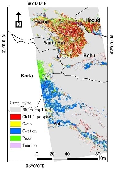
Remotesensing 12 00158 g009
Figure 10. Crop distribution map of the study area derived from random forest (RF) classification using the combined Sentinel-1 and Sentinel-2 feature set.
Remotesensing 12 00158 g010
Figure 11. A subset of VH intensity on 26 March 2018 extracted from (a) Original synthetic aperture radar (SAR) intensity; (b) SAR intensity filtered by the refined Lee method; (c) SAR intensity filtered by the SHP distributed scatterer interferometry (DSI) method.
Remotesensing 12 00158 g011
Figure 12. A subset of VV coherence on 7 April 2019 extracted from (a) Coherence coefficient estimated by a 7 × 7 sliding window; (b) Coherence coefficient estimated by the SHP DSI method with bias mitigation.
Remotesensing 12 00158 g012
Figure 13. Comparison of crop type mapping results using different feature combinations. Four groups of features were tested, the first group contains only SAR (Sentinel-1) features, the second group contains only optical (Sentinel-2) features without the red-edge contribution, the third group has all of the Sentinel-2 features, the fourth group includes both SAR and optical (Sentinel-1 and 2) features.
Remotesensing 12 00158 g013
Figure 14. Accumulated feature importance scores of features selected for (a) step 1: cropland extraction and (b) step 2: crop type discrimination, calculated for each subcategory regardless of acquisition time. Each importance score was normalized and converted to a percentage. Each feature is named by its subcategory and acquisition time in the format of “yyyymmdd”.
Remotesensing 12 00158 g014
Figure 15. The accumulated importance scores of features selected in step 1: cropland extraction in three groups. The first group contains only Sentinel-1 features; the second group comprises only Sentinel-2 features exclusive of the red-edge features; the third group includes only the red-edge features. (a) Feature scores in the three groups calculated regardless of the acquisition time; (b) Feature scores in the three groups calculated for each month. The VH amplitude dispersion, as a single-phase feature, is plotted on the rightmost bar. Each importance score was normalized and converted to a percentage.
Remotesensing 12 00158 g015
Figure 16. The accumulated importance scores of features selected in step 2: crop type discrimination in three groups. The first group contains only Sentinel-1 features; the second group comprises only Sentinel-2 features exclusive of the red-edge features; the third group includes only the red-edge features. (a) Feature scores in the three groups calculated regardless of the acquisition time; (b) Feature scores in the three groups calculated for each month. The VH amplitude dispersion, as a single-phase feature, is plotted on the rightmost bar. Each importance score was normalized and converted to a percentage.
Remotesensing 12 00158 g016
Figure 17. Heat maps showing correlation between selected features. (a) Correlation heat map of selected features in step 1; (b) correlation heat map of selected features in step 2. In both (a,b), the feature indexes follow the feature rankings obtained through the RF feature importance score. Correlation close to 1 or −1 indicates high positive or negative correlation between features. The diagonal elements in both correlation matrices are self-correlation coefficients, so they constantly equal one. (c) The histogram of correlation between selected features in step 1; (d) the histogram of correlation between selected features in step 2. In both (c,d), the histograms were calculated after removing the diagonal elements of the correlation matrices and converting a negative correlation coefficient to corresponding positive values. Thus, the ‘0’ in the histogram indicates low correlation, while ‘1’ indicates high correlation.
Remotesensing 12 00158 g017
Figure 18. Boxplots of selected VH intensity features of different crop types, spanning the time from 26 March 2018 to 13 May 2018, as well as a feature on 16 October 2018. Each feature is named by its subcategory and acquisition time in the format of “yyyymmdd”. In (ae), pear values show an apparent distinction from other crops, while in (f), chili can be easier recognized.
Remotesensing 12 00158 g018
Figure 19. Boxplots of the top three scoring master versus slave VH intensity ratio of different crop types. Each feature is named by its subcategory and acquisition time in the format of “yyyymmdd”. (a) Boxplots of the master vs. slave VH intensity ratio derived from the 29 August 2018 acquisition of Sentinel-1; (b) boxplots of the master vs. slave VH intensity ratio derived from 10 September 2018 acquisition of Sentinel-1; (c) boxplots of the master vs. slave VH intensity ratio derived from 4 October 2018 acquisition of Sentinel-1.
Remotesensing 12 00158 g019
Figure 20. Boxplots of selected SAR features of different crop types. (a) Coherence coefficient in VV polarization mode; (b) amplitude dispersion in VH polarization mode. Each feature is named by its subcategory and acquisition time in the format of “yyyymmdd”.
Remotesensing 12 00158 g020
Figure 21. Boxplots of selected red-edge indices showing a good capability to distinguish corn from other crops. Each feature is named by its subcategory and acquisition time in the format of “yyyymmdd”. (a) Boxplots of the NDVIre2n indices derived from the 1 September 2018 acquisition of Sentinel-2; (b) boxplots of the NDVIre2n indices derived from the 17 August 2018 acquisition of Sentinel-2; (c) boxplots of the CIre indices derived from the 17 August 2018 acquisition of Sentinel-2; (d) boxplots of the NDVIre1n indices derived from the 17 August 2018 acquisition of Sentinel-2; (e) boxplots of the MSRre indices derived from the 17 August 2018 acquisition of Sentinel-2; (f) boxplots of the NDre2 indices derived from the 17 August 2018 acquisition of Sentinel-2; (g) boxplots of the NDVIre2 indices derived from the 17 August 2018 acquisition of Sentinel-2; (h) boxplots of the MSRren indices derived from the 17 August 2018 acquisition of Sentinel-2; (i) boxplots of the NDVIre2 indices derived from the 01 September 2018 acquisition of Sentinel-2.
Remotesensing 12 00158 g021
Figure 22. Boxplots of selected red-edge indices revealing a clear distinction between the pear and other crops. Each feature is named by its subcategory and acquisition time in the format of “yyyymmdd”. (a) Boxplots of the NDVIre1 indices derived from the 9 May 2018 acquisition of Sentinel-2; (b) boxplots of the NDVIre1n indices derived from the 6 October 2018 acquisition of Sentinel-2; (c) boxplots of the NDVIre2 indices derived from the 9 May 2018 acquisition of Sentinel-2; (d) boxplots of the CIre indices derived from the 06 October 2018 acquisition of Sentinel-2.
Remotesensing 12 00158 g022
Figure 23. Boxplots of selected red-edge features showing good separability of chili pepper. Each feature is named by its subcategory and acquisition time in the format of “yyyymmdd”. (a) Boxplots of the band 6 values from the 17 August 2018 acquisition of Sentinel-2; (b) boxplots of the band 6 values from the 1 September 2018 acquisition of Sentinel-2; (c) boxplots of the band 7 values from the 17 August 2018 acquisition of Sentinel-2.
Remotesensing 12 00158 g023
Table 1. Phenological calendars of the major crop types in the study site.
JanFebMarAprMayJunJulAugSepOctNovDec
Cotton △☆☆√
Corn (Spring) △☆☆√
Corn (Summer) △☆
Pear
Chili pepper ★☆☆√
Tomato ★☆
Legend: △ Sowing; ♤ Budding; ♠ seedling nurturing; ★ Transplanting; ☆ Growing; √ Harvesting.
Table 2. Ground samples of the six land cover types in the study area.
Land Cover TypeSample Points
Cropland3817
Forest1468
Desert1468
Urban area2349
Waterbody3257
Wetlands3125
Table 3. Ground samples collected for major crop types in the study area.
Crop TypeFoldTraining SamplesTesting Samples
No. of FieldsNo. of Points PointsNo. of FieldsNo. of Points
Chili pepper1st571481837
2nd501472538
3rd68147738
4th631511234
5th71147438
Corn1st2389922
2nd2588723
3rd3090221
4th2987324
5th21901121
Cotton1st371501338
2nd43151737
3rd43152736
4th341511637
5th43152736
Pear1st2276219
2nd2078417
3rd1576919
4th1877618
5th2173322
Tomato1st19104231
2nd16108527
3rd19108227
4th15110625
5th15110625
Table 4. The employed Sentinel-1 and Sentinel-2 acquisitions of each month.
Acquisition TimeMarAprMayJunJulAugSepOct
Sentinel-1A12333322
Sentinel-2A00100111
Sentinel-2B00011011
Table 5. Metadata of the data stack of Sentinel-1 (S1) interferometric wide swath (IW) single look complex (SLC) data using the parameters from the first image. These values remain very close for all subsequent acquisitions.
Sentinel-1 IW SLC Data
First acquisition26 March 2018
Last acquisition16 October 2018
Pass directionAscending
Polarization modeVV + VH
Incidence angle (°)36.12–41.84
Wavelength (cm)5.5 (C-band)
Range spacing (m)2.33
Azimuth spacing (m)13.92
Table 6. Central wavelength and bandwidth of different spectral bands of Sentinel-2 data used in this research.
Spatial Resolution (m)Spectral BandsS2AS2B
Central Wavelength (nm)Central Wavelength (nm)
10B2Blue496.6492.1
B3Green560559
B4Red664.5665
B8Near-infrared (NIR)835.1833
20B5Red-edge 1703.9703.8
B6Red-edge 2740.2739.1
B7Red-edge 3782.5779.7
B8ANIR narrow864.8864
B11Short-wave infrared (SWIR) 11613.71610.4
B12SWIR 22202.42185.7
Table 7. Spectral indices calculated from Sentinel-2 data.
Reference Spectral IndicesFormula
NDVINormalized Difference Vegetation Index N D V I = ( B 8 B 4 ) ( B 8 + B 4 )
NDWINormalized Difference Water Index N D W I = ( B 3 B 8 ) ( B 3 + B 8 )
Red-edge spectral indicesFormula
NDVIre1Normalized Difference Vegetation Index red-edge 1 [32] N D V I r e 1 = ( B 8 B 5 ) ( B 8 + B 5 )
NDVIre1nNormalized Difference Vegetation Index red-edge 1 narrow [6] N D V I r e 1 n = ( B 8 a B 5 ) ( B 8 a + B 5 )
NDVIre2Normalized Difference Vegetation Index red-edge 2 [6] N D V I r e 2 = ( B 8 B 6 ) ( B 8 + B 6 )
NDVIre2nNormalized Difference Vegetation Index red-edge 2 narrow [6] N D V I r e 2 n = ( B 8 a B 6 ) ( B 8 a + B 6 )
NDVIre3Normalized Difference Vegetation Index red-edge 3 [32] N D V I r e 3 = ( B 8 B 7 ) ( B 8 + B 7 )
NDVIre3nNormalized Difference Vegetation Index red-edge 3 narrow [6] N D V I r e 3 n = ( B 8 a B 7 ) ( B 8 a + B 7 )
CIreChlorophyll Index red-edge [33] C I r e = B 7 B 5 1
NDre1Normalized Difference red-edge 1 [32] N D r e 1 = ( B 6 B 5 ) ( B 6 + B 5 )
NDre2Normalized Difference red-edge 2 [34] N D r e 2 = ( B 7 B 5 ) ( B 7 + B 5 )
MSRreModified Simple Ratio red-edge [35] M S R r e = ( B 8 / B 5 ) 1 ( B 8 / B 5 ) + 1
MSRrenModified Simple Ratio red-edge narrow [6] M S R r e n = ( B 8 a / B 5 ) 1 ( B 8 a / B 5 ) + 1
Table 8. Accuracy of step 1 land cover classification, assessed by stratified 10-fold cross-validation using the ground samples. OA: overall accuracy.
Mean OA (%)Kappa CoefficientF1 Score
94.05%0.927Cropland0.942
Forest0.835
Desert0.908
Urban area0.932
Waterbody0.995
Wetlands0.945
Table 9. Accuracy of step 2 crop type classification using the optimal combination of S1 and S2 features, assessed by stratified fivefold cross-validation using the ground samples.
Mean OA (%)Kappa CoefficientF1 Score
86.98%0.83Chili pepper0.84
Corn0.71
Cotton0.97
Pear0.94
Tomato0.79
Table 10. Accuracy of step 2 crop type classification using the optimal combination of S1 and S2 features, assessed by stratified fivefold cross-validation using one sample from each validation field.
Mean OA (%)Kappa CoefficientF1 Score
83.22%0.77Chili pepper0.87
Corn0.69
Cotton0.91
Pear0.89
Tomato0.71
Table 11. Accuracy metrics of crop type classification using SAR features processed by different filters. SHP: statistically homogeneous pixel.
Mean OAKappa CoefficientF1-Score ChiliF1-Score CornF1-Score CottonF1-Score PearF1-Score Tomato
Original60.20%0.480.550.330.670.720.58
Refined Lee73.21%0.650.660.520.800.830.74
SHP DSI79.46%0.730.750.600.880.860.77
Table 12. Accuracy assessment of crop type discrimination using different groups of features. The mean overall accuracy (OA) and kappa coefficient were averaged over fivefold cross-validation in both multi-sample per field validation and one sample per field validation.
Optimal Number of FeaturesMean OAKappa Coefficient
Multi Samples per FieldOne Sample per FieldMulti Samples per FieldOne Sample per Field
Sentinel-113379.46%76.91%0.730.69
Sentinel-2 without red-edge features5882.37%79.80%0.770.72
Sentinel-210485.43%81.64%0.810.75
Sentinel-1 and Sentinel-211386.98%83.22%0.830.77

