Abstract
Supervised classification methods, used for many applications, including vegetation mapping require accurate “ground truth” to be effective. Nevertheless, it is common for the quality of this data to be poorly verified prior to it being used for the training and validation of classification models. The fact that noisy or erroneous parts of the reference dataset are not removed is usually explained by the relatively high resistance of some algorithms to errors. The objective of this study was to demonstrate the rationale for cleaning the reference dataset used for the classification of heterogeneous non-forest vegetation, and to present a workflow based on the t-distributed stochastic neighbor embedding (t-SNE) algorithm for the better integration of reference data with remote sensing data in order to improve outcomes. The proposed analysis is a new application of the t-SNE algorithm. The effectiveness of this workflow was tested by classifying three heterogeneous non-forest Natura 2000 habitats: Molinia meadows (Molinion caeruleae; code 6410), species-rich Nardus grassland (code 6230) and dry heaths (code 4030), employing two commonly used algorithms: random forest (RF) and AdaBoost (AB), which, according to the literature, differ in their resistance to errors in reference datasets. Polygons collected in the field (on-ground reference data) in 2016 and 2017, containing no intentional errors, were used as the on-ground reference dataset. The remote sensing data used in the classification were obtained in 2017 during the peak growing season by a HySpex sensor consisting of two imaging spectrometers covering spectral ranges of 0.4–0.9 μm (VNIR-1800) and 0.9–2.5 μm (SWIR-384). The on-ground reference dataset was gradually cleaned by verifying candidate polygons selected by visual interpretation of t-SNE plots. Around 40–50% of candidate polygons were ultimately found to contain errors. Altogether, 15% of reference polygons were removed. As a result, the quality of the final map, as assessed by the Kappa and F1 accuracy measures as well as by visual evaluation, was significantly improved. The global map accuracy increased by about 6% (in Kappa coefficient), relative to the baseline classification obtained using random removal of the same number of reference polygons.
1. Introduction
Reference data used for the supervised classification of vegetation are collected in a number of different ways. Both archival on-ground-based data, collected for other purposes, and data acquired during field campaigns, specifically for the purpose of classification, are used equally often [1,2]. Data gathered based on the photointerpretation of a high-resolution orthophoto map are used less frequently [3]. Regardless of the method used to collect reference data, they may contain errors, even those acquired by authoritative sources [4]. Errors in the data may result from various factors, one of which being differences in the methods used for the identification of vegetation type when they come from different sources and when they were collected for different purposes [1]. In this case, the problem may arise from both a different interpretation of a given vegetation type by individual researchers, and the determination of vegetation units at different hierarchy levels (upper hierarchy level = higher level of generality). Errors in the reference dataset can also be caused by errors in the positioning of a given reference sample, for example, using a low accuracy GNSS based technique [5]. In such a case, the reference sample can be established outside a given vegetation type or at the transition zone between two types, resulting in its internal heterogeneity and mixed pixels [5]. Errors may also result from incorrect labeling of a given vegetation type in the database [4]. A low quality of reference data may also be associated with differences between the time at which the remote sensing data and on-ground reference data were acquired [3], especially when the reference data are acquired before the acquisition of remote sensing data. In such a case, the given type of vegetation at the location of a reference sample could be transformed to another type of vegetation or destroyed in the period between the acquisition of on-ground reference botanical data and remote sensing data. In addition to the above, there are other factors that have a negative impact on the quality of reference data, such as those related to the poorer quality of the raster data at a given location of reference samples.
It has been repeatedly emphasized by other authors that the quality of training data significantly influences the results of a supervised classification [6,7,8,9]. Training data class mislabeling, or noise, often negatively affects the outcome of machine learning algorithms [10]. Unfortunately, in many studies, the quality of training data is not checked and reference data are therefore used directly for model training, without any initial analysis of correctness [8]. One can observe that much more attention is paid to sampling design, sample size and training data class imbalance than to the quality of the reference data itself [8]. This is a bad practice, which may have crucial consequences for the quality of classification results, especially when mapping several classes of similar types of vegetation. In this case, errors in classes with similar spectral characteristics will have a significantly greater negative impact on the classification results than those involving spectrally different land-cover categories [1]. This kind of situation often occurs in the classification of non-forest vegetation, where patches of different types of vegetation may be composed of the same dominant species, have similar physiognomy and, at the same time, occur in the immediate vicinity. In such situations, the boundary between two types of vegetation is often difficult to identify, which can hinder the correct establishment of a reference sample. Furthermore, this boundary may shift and change in size from year to year, due to changes in land use and various natural factors affecting the species composition of a given type of vegetation [11].
According to the authors of [2], an improvement in the quality of the training set usually results in an improvement in the classification results. Hitherto, several methods have been proposed to assess quality and to identify and remove outlying observations. The quality of the reference data can be assessed indirectly by analyzing results from the error matrix after the classification procedure and directly before the classification procedure using various indices. For this purpose, the following measures are used: distances—e.g., k-nearest neighbor (k NN) [12], isolation forest (iForest) [13] and the local outlier factor [14]; the similarity measure—using random forest (RF) for this purpose [9]; and measures based on the rough sets theory [8]. Some methods also use an iterative training-classification scheme [15]. It is also possible to use visualization tools to evaluate samples contained in the reference data; for this purpose, the authors of [16] used the nonlinear mapping technique described in [17], as here it was used for projecting the 12-dimensional space of objects into the subspace of two and three dimensions, which allowed for the elimination of atypical and mixed pixels.
A new, simple expert method based on the t-distributed stochastic neighbor embedding (t-SNE) algorithm, known from other applications [18], is proposed in this work in order to improve the reference dataset by efficient detection of potential errors by visual analysis of t-SNE plots. t-SNE is a nonlinear dimension reduction technique that enables the visualization of high-dimensional data by giving each data-point a location in a two or three-dimensional map. The t-SNE models each multidimensional sample in such a way that similar samples are represented by nearby points, whilst different samples are represented by distant points. The selected algorithm has a number of significant advantages over other visualization techniques. Since it is designed for the visualization and reduction of multidimensional data, it is capable of capturing the local structure of high-dimensional data very well, whilst revealing global structure, such as the presence of clusters, at several scales. In addition, the tendency to concentrate points in the middle of the visualization—a major drawback of other visualization techniques—is significantly reduced [18]. The t-SNE algorithm is used for visualization in a wide range of applications and recent reports indicate that the algorithm can be successfully used for remote sensing data, for example to extract features in order to improve classification results [19,20,21]. This algorithm is particularly applicable to the classification of hyperspectral data, in which the reduction of data dimensionality is very important, due to the commonly known Hughes’ Phenomenon [20,22]. Posed as a hypothesis that the correctness of the reference dataset has a crucial impact on classification outcomes, the objective of this study was to assess the effectiveness of the t-SNE algorithm for the elimination of errors in the on-ground botanical reference dataset used to classify selected types of non-forest vegetation. This approach was developed and applied during the HabitARS project [23,24].
The research was conducted in Central Poland. Three non-forest Natura 2000 habitats and surrounding vegetation (background) co-occurring in the Natura 2000 area “Dolina Krasnej” (Krasna Valley) were selected as the subject of this research. The selected Natura 2000 habitats have a number of features, which may significantly hinder their correct classification by remote sensing methods. First of all, each of them may be subject to varied agricultural use or overgrown by shrubs and trees as a result of succession. Secondly, they may be characterized by either a high similarity of species composition between other analyzed Natura 2000 habitat classes or other vegetation types (background class), or a high degree of floristic diversity within a given class. In addition, in many cases, they form patches with transitional characteristics and often coexist with each other in a given location. They may also undergo transformations into a different type of vegetation (both into other analyzed Natura 2000 habitat classes and the background class) even from year to year. On-ground reference data were collected with the utmost care, so they should be close to “ground truth”. However, the reference data were collected over an extended time period, which could also be a source of potential errors.
Airborne hyperspectral data were used as the basis of a remotely sensed dataset for classification. The type of imagery has demonstrated sufficient spectral resolution to classify these types of land cover classes characterized by subtle differences in spectral characteristics [25]. Two classification algorithms were used to perform the classification: random forest (RF) and AdaBoost (AB). Both are decision tree-based ensemble classifiers, widely used in remote sensing studies. Additionally, the RF has a reputation for being relatively resistant to the presence of noise in training data [3,9,26,27]. Conversely, a number of references indicate AB has a lower resistance [28,29,30]. Apart from the commonly used accuracy measures, a visual assessment of the resulting maps was carried out to assess the results of classification. The use of two different classification algorithms and an additional botanical assessment allowed us to thoroughly assess the utility of the proposed method of quality improvement by modification of the on-ground reference dataset.
2. Materials and Methods
2.1. Study Area and Object of the Study
The research was conducted in Central Poland at the Natura 2000 site “Dolina Krasnej” (code PLH260001; Figure 1). The site covers a natural marshy valley of the Krasna River and its tributaries.
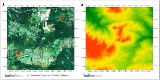
Figure 1.
Location of the study area. Left side: basemap: HySpex image in natural color red, green, blue (RGB) composition with on-ground polygon locations (red circles). Right side: digital elevation model.
The study area is largely covered with forests, but at the same time is characterized by exceptionally high heterogeneity of non-forest vegetation. The area also features complexes of various types of meadows, grasslands, mires and rush vegetation. The most valuable components of this area include, inter alia, non-forest Natura 2000 habitats analyzed within the scope of this paper (Table 1): Molinia meadows on calcareous, peaty or clayey-silt-laden soils (Molinion caeruleae; code 6410), species-rich Nardus grassland on siliceous substrates in mountain areas (and sub-mountain areas in continental Europe; code 6230) and European dry heaths (code 4030). These are described in detail in Table 1.

Table 1.
Characteristics of the analyzed Natura 2000 habitats in the study area.
2.2. Data Acquisition
2.2.1. On-Ground Reference Data
On-ground reference data were collected during the growing seasons of 2016 and 2017 (Table 2). The unit of reference polygons was a circle with a radius of 3 m. In exceptional situations, when the habitat patches were small, the radius was reduced. The geolocation of reference polygons was recorded using a GNSS Mobile Mapper 120 (with real-time differential correction) yielding a measurement accuracy from 0.5 to 0.2 m. Data were collected for three Natura 2000 habitats with codes: 6410, 6230 and 4030, as well as for all other forest and non-forest types of vegetation (also mown) representing the so-called background class. In addition, the database was supplemented with polygons of the background class digitized on red–green–blue (RGB) and infra-red (CIR) orthophoto maps, referred to as “water”, “forest” and “non-forest vegetation in shadow” (30 per subclass). The polygons were established in such a way as to represent all the variability of the analyzed Natura 2000 habitats and the background in the study area. Detailed information on co-occurring species with a cover of more than 20% was recorded for every Natura 2000 habitat polygon. The percentage contribution of specific components (bare soil, vegetation, moss and lichen cover, and the presence of necromass) as well as the land use (no use, mowing, and grazing) were also recorded. The type of vegetation and species that covered more than 50% of the polygon’s area were recorded for the background polygons. Such detailed information enabled us later to interpret and thoroughly verify the polygons selected as potentially containing errors, after visual interpretation of t-SNE results. In total, 1476 spatially non-overlapping reference polygons (containing 47 232 pixels) were established (Table 2). On-ground reference data collected in different periods were merged into one on-ground reference dataset.

Table 2.
Statistics related to on-ground botanical measurements.
2.2.2. Remote-Sensing Data Acquisition
The time frame for remote sensing data acquisition was specified based on the optimum development of the analyzed Natura 2000 habitats. The hyperspectral data were obtained on 7 July 2017 with a HySpex sensor developed by the Norwegian Norsk Elektro Optikk (NEO) company. It is part of a remote sensing platform built within the framework of the HabitARS project by the MGGP Aero Company [31]. The data were acquired for an area of 40.59 km2. The HySpex instrument was flown on board the Cessna CT206H at an average altitude of 730 m above ground level (AGL) and an airspeed of 59.2 m/s. The HySpex sensor consists of two imaging spectrometers covering spectral ranges of 0.4–0.9 μm (VNIR-1800) and 0.9–2.5 μm (SWIR-384). The number of flight lines was 25 and the flight orientation was west-east.
In the next stage, the acquired raw data were preprocessed in accordance with the methodology presented in Sławik et. al 2019 (Subdivision 2.3.1) [31]. The hyperspectral mosaics were subjected to a minimum noise fraction transformation (MNF). The first 30 bands resulting from the transformation were selected basing on MNF eigenvalues and used in the analysis. This analysis was performed using ENVI version 5.4 (Broomfield, CO, USA) [32]. The initial reduction of data dimensionality is recommended as it significantly improves the performance of both the t-SNE [18] and the classification algorithms [33].
2.3. Analysis Workflow
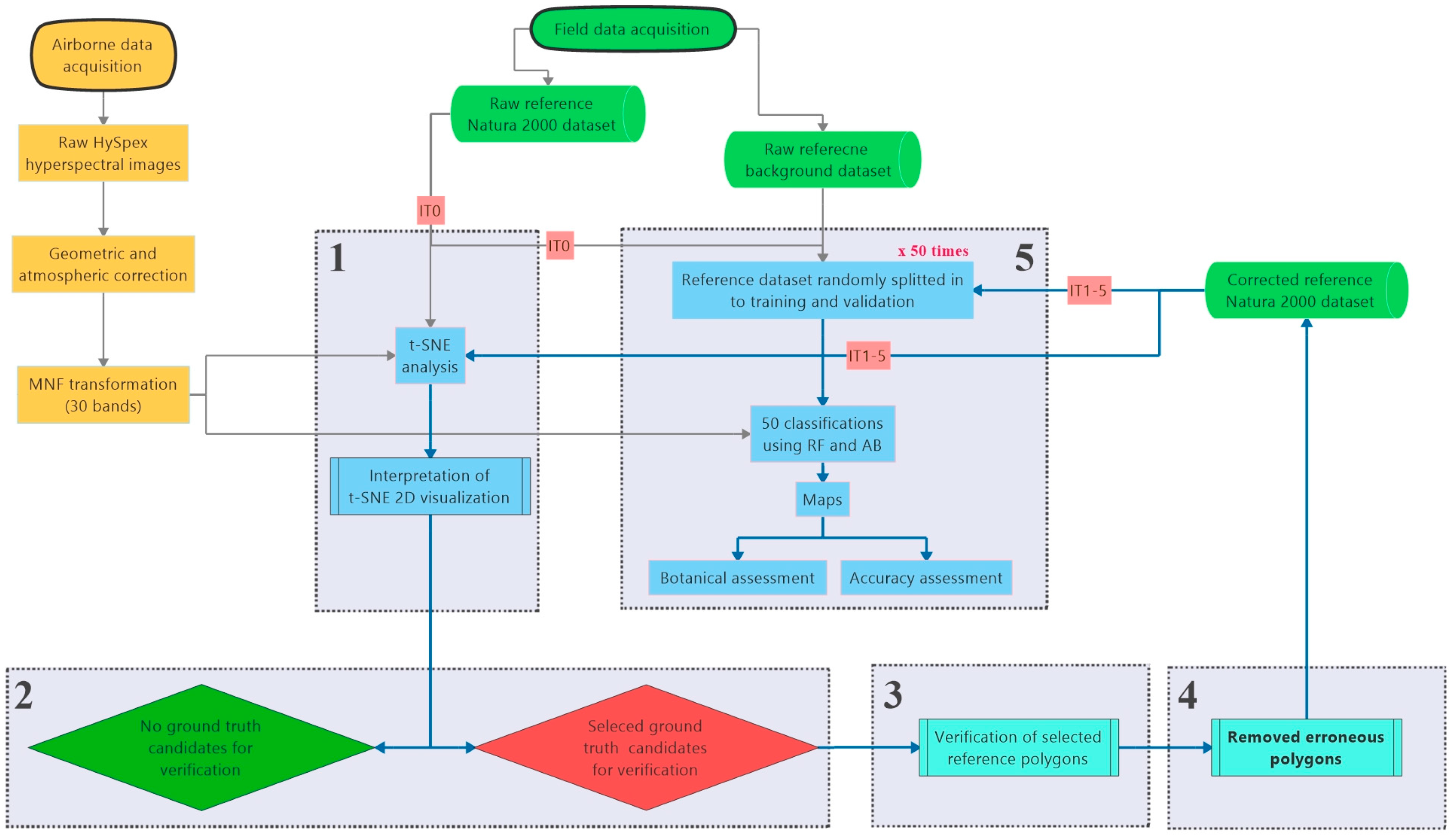
The method of conducting and interpreting the t-SNE analysis was based on hitherto published reports [18,34] and our earlier experience in HabitARS project [11]. The exact workflow is presented in Figure 2 and the detailed description of the methods used during each stage is presented in the Section 2.3.1, Section 2.3.2, Section 2.3.3, Section 2.3.4 and Section 2.3.5.
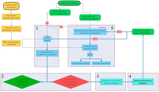
Figure 2.
Workflow of the conducted analyses. Stages 1–5 is repeated in each iteration.
t-SNE visualizations and classifications were performed using the Vegetation Classification Studio (VCS) software [35], which is a tool for comprehensive classification and analysis of vegetation based on remote sensing data. The t-SNE analysis is one of the VCS standard functions, which can be invoked by configuring a set of parameters in the VCS YAML-based session definition file. The session file indicates locations of vector and raster datasets to use, types of analysis, classification settings and the set of reports to generate. The t-SNE-related parameters allow for generating visualizations with a set of different perplexity values, which in this case can be interpreted as a measure of the effective number of neighbors [18], as well as using a “stable initialization" by starting the algorithm with principal component analysis (PCA)-transformed data—a very useful feature to support visual analysis and comparison of multiple visualizations of the same dataset.
The main activities of the workflow were performed iteratively. Each iteration consists of the following stages: (1) generation and visual analysis of t-SNE plots, (2) selecting candidate ground truth polygons for verification, (3) verification of selected reference polygons and removal of reference that was found erroneous, (4) classification using modified and baseline reference and (5) botanical assessment of classification results.
The initial iteration (IT0) of the workflow started with the classification performed on the original, on-ground reference dataset (1476 polygons). Final number of iterations was not planned in advance and it was intended for this process to continue until we could not detect more errors in any of the analyzed Natura 2000 habitat classes; this state was reached after 5 iterations (IT5).
2.3.1. Generating t-SNE Based Visualization of Reference Dataset
For each on-ground reference polygon, the input vector consisted of all pixels located within a given polygon, with values coming from all 30 MNF channels. Since t-SNE works with relative distances between multi-dimensional data points and does not perform any normalization or scaling internally, all MNF channel values were scaled to the same range; thus the full range of values for every MNF band had the same impact when calculating the effective distances between samples.
The analysis in IT0 started by generating a series of t-SNE visualizations on the unmodified dataset with different perplexity. The purpose here was to find the perplexity value which maximized usability of visualizations to detect relevant features of the on-ground reference dataset. All subsequent analyses were carried out with this optimum perplexity value. Also, to facilitate comparison of multiple visualizations of the same dataset throughout the analysis, the function of “stable initialization” was used.
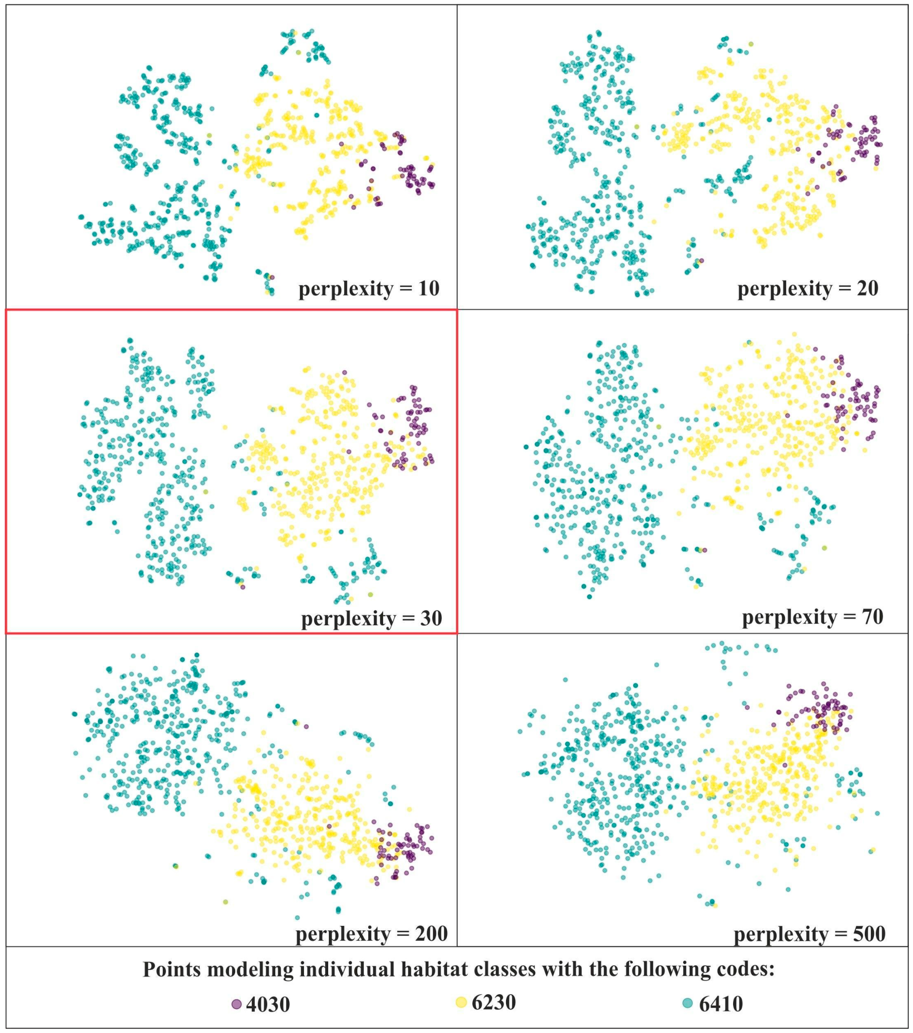
In order to select optimal perplexity values for further analysis, a series of t-SNE visualizations was performed on the unmodified dataset with the following perplexity values: 10, 20, 30, 40, 50, 60, 70, 80, 90, 100, 150, 200, 500, 1000. The analysis of the usefulness of the resulting visualizations involved a trade-off between preserving local and global structure. As we can see, lower values of perplexity emphasize the local structure, whilst higher values of perplexity are better at preserving the global structure (Figure 3). Perplexity values in the range of 30–70 yielded comparatively good visualizations. However, bearing in mind that the best perplexity settings are influenced by, among others, the total number of samples [18,34] and this number may decrease significantly during subsequent iterations of the analyses, the perplexity value equal to 30 was selected (Figure 3).
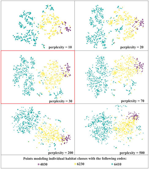
Figure 3.
t-SNE visualizations for three Natura 2000 habitats—code 4030, 6410 and 6230 using different perplexity values on unmodified on-ground reference dataset (IT0). For further visualizations the perplexity value of 30 was selected (red frame).
2.3.2. Visual Interpretation of t-SNE Plots to Select Candidate Polygons for Verification
The selection of potential errors in the on-ground reference dataset using the t-SNE algorithm was carried out only for the three selected Natura 2000 habitats. The background class polygons were excluded from these analyses, because they belonged to heterogeneous classes of vegetation, characterized by varying spectral features.
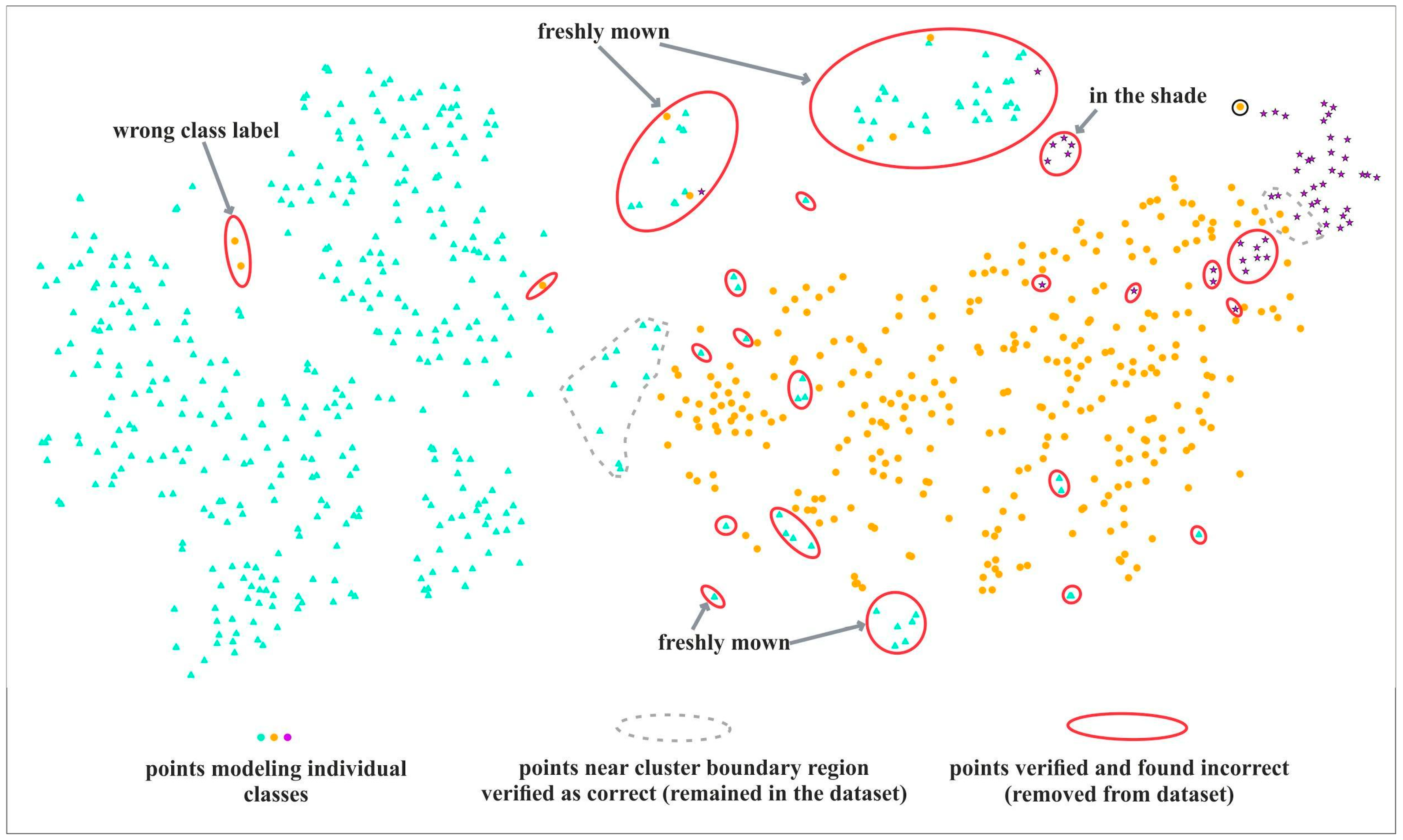
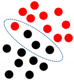
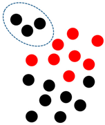
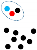
The example t-SNE image (Figure 4) shows points representing on-ground reference polygons. The points are colored according to their classes, and laid out in space to form different groups and clusters. In an ideal case, all points belonging to a class should form a clearly distinct cluster. Typically, we can see one or more dominant clusters, a number of smaller ones, with various amounts of mixing and outliers. The t-SNE algorithm tries to preserve distances between points, so the points that are close by in the visualization typically have similar spectral properties.
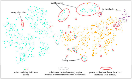
Figure 4.
Interpretation of t-SNE visualization. A red solid line indicates confirmed errors, removed from the on-ground reference dataset after verification of causes. Some error types are indicated by the arrows. A grey dotted line shows examples of candidate points near boundary regions, selected for verification, that were ultimately found to be correct and remained in the database.
Table 3 lists typical examples of visualization patterns we were looking for in our plots, and the resulting underlying interpretation in the reference database. When we detected one of those suspicious visual patterns, we selected relevant points and they were subject to verification in the next stage.

Table 3.
List of visual analysis artifacts and how they translate into potential reasons/effects in reference database.
The visual interpretation of t-SNE plots did not take into account absolute positions of points or their clusters in the xy space, because—due to the properties of t-SNE algorithm—each subsequent visualization (even generated from the same input data and parameters) could result in a slightly different arrangement of objects in space. In addition, in general, inferring the absolute degree of similarity between points and clusters using this approach is quite limited and only possible with careful selection of the perplexity value. One class could be represented as a single cluster or many smaller clusters. However, this did not have to prove of internal diversity of a given class and could be dependent on parameters used in the calculations, i.e., perplexity [18,34].
2.3.3. Verification of Candidate Ground Truth Polygons and Removal of Erroneous Reference
The next step consisted of careful checking and verification of selected ground truth polygons using all available reference data, notes, photos and other information collected in the field as well as photointerpretation of the HySpex RGB and CIR composites.
The most obvious type of error was just wrong class label assigned to a polygon. Note that—to be consistent with our preset methodology—we removed such errors from the database, while in almost any practical settings, such errors should be corrected. Another common case were polygons incorrectly selected to represent a class, due to the transitional nature of vegetation. Another common cause of errors were polygons that were collected properly, but located in areas covered by shadow in remote sensing data. Many cases of polygons were found in areas mown in the period between remote sensing and botanical data collections. A few cases were overgrown by trees or shrubs or having other issues which prevented them from being representative for their intended class.
All reference polygons identified as errors were permanently removed from the database. Many candidate polygons were found to be correct, and they remained intact in the database until the next iteration.
2.3.4. Classification and Validation
Classifications were carried out to assess the effects of the modification of the on-ground reference dataset (after each t-SNE analysis) on the resultant map and classification accuracy measures (Step 1). For this study, random forest (RF) and AdaBoost (AB) classifiers were used, due to their popularity and representativeness for respective groups of algorithms, based on bagging or boosting approaches respectively. In addition, the selected classifiers in their resistance to the presence of noisy observation data, with the RF classifier considered as one of the most resistant algorithms [3,9,27,28].
In each iteration, two classifications (using both RF and AB) were made. The first was a direct classification based on reference corrected during the iteration. The other one was classification used as baseline to better compare the effect our fixes to the reference database. This baseline classification was created by randomly removing the same number of polygons of each class that were eliminated from the reference. So for each reference polygon removed by our workflow in a given iteration, we removed one randomly selected polygon from our baseline classification. The aim of this procedure was to better assess the effects of removing reference by our workflow compared to a random removal of same number of polygons. That also makes the classification accuracies more representative and comparable between iterations.
Each classification was repeated 50 times, each time the dataset was randomly split into training and validation polygons in 50:50 ratio. For each result, accuracy was characterized using the Cohen’s Kappa coefficient [36] and the F1 score [6]. Accumulated accuracy measures, including user’s accuracy (UA) and producer’s accuracy (PA), were calculated for each set of 50 classifications. To produce raster map of the study and analyze detailed accuracy reports (e.g., confusion matrix) the model with median accuracy (1 of 50) was selected. The numbers of pixels in confusion matrices were converted into a percentage to facilitate the interpretation of these results.
2.3.5. Botanical Assessment of Classification Products (Maps)
Apart from the statistical comparison of the standard accuracy measures, a botanical assessment was carried out by experts who collected the on-ground reference polygons. The analysis involved a visual botanical assessment of the classification results on orthophoto maps using RGB and CIR composites. Only the maps from the first (IT0) and last (IT5) iterations were compared.
Spectral reflectance curves were constructed from pixels of on-ground reference polygons to compare the spectral distinctiveness of analyzed Natura 2000 habitat classes and the background class. The curve for each Natura 2000 habitat was constructed as an average of 30 pixels (one middle pixel for each of the 30 on-ground reference polygons). Two spectral reflectance curves were created for each Natura 2000 habitat. The first one was created from both erroneous polygons (removed during later iterations) and correct polygons. The second spectral reflectance curve was created only from polygons that remained intact in our database after all iterations. In addition, spectral reflectance curves were constructed for pixels where specific disturbance factors, such as shadow or mowing, were present.
3. Results
3.1. Results of the t-SNE Analysis
In total, six iterations (IT0–IT5) of our workflow were carried out; thus, the size of the on-ground reference dataset was reduced five times. The visualization obtained in the last iteration of the analysis did not reveal the presence of artifacts, therefore the analysis was not continued (Figure 5). The IT0 was performed on the full (unmodified) on-ground reference dataset. This resulted in detection of the largest number of erroneous polygons (133); these were both mixed with other classes of Natura 2000 habitats and located in isolation from all of the analyzed classes (Figure 5, Table 4). Some points were quite clearly lying in unexpected places, and a lot of them were found to be incorrect after verification. On the other hand, for points lying in boundary regions, especially near intersection between two habitat classes, many of them were found correct, and thus remained in the database. At the later stages of the analysis, the number of artifacts was significantly smaller, ranging from 14 (based on the visualization at the IT2) to 35 (based on the IT4). In total, as a result of the iterative t-SNE analysis, 216 erroneous polygons were detected and removed, which accounted for 25% of the set containing on-ground reference polygons of Natura 2000 habitats (without on-ground reference polygons representing the background) and 15% of the entire on-ground reference dataset. Most erroneous polygons were removed from class with code 6410 and the least from class with code 4030 (Table 4). On the other hand, in terms of the percentage loss, the class with code 4030 lost 63% of its polygons and class 6410—27%, and class 6230—14%.
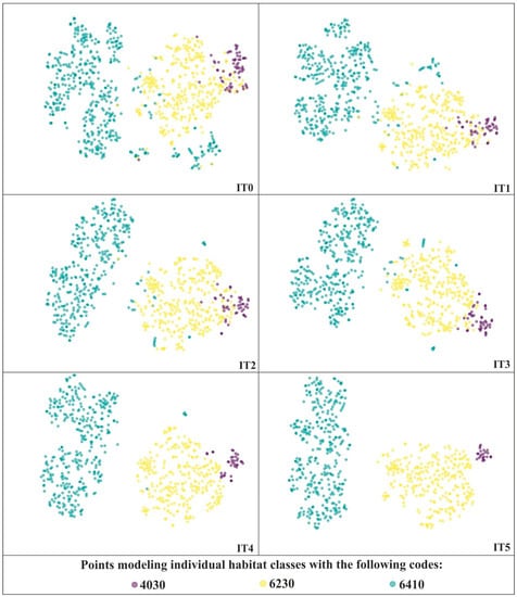
Figure 5.
The t-SNE visualizations for three Natura 2000 habitats—code 4030, 6410 and 6230 performed during successive iterations of the analyses.

Table 4.
The number of polygons of particular Natura 2000 habitats in individual iterations of the analyses together with a summary of the number of removed polygons.
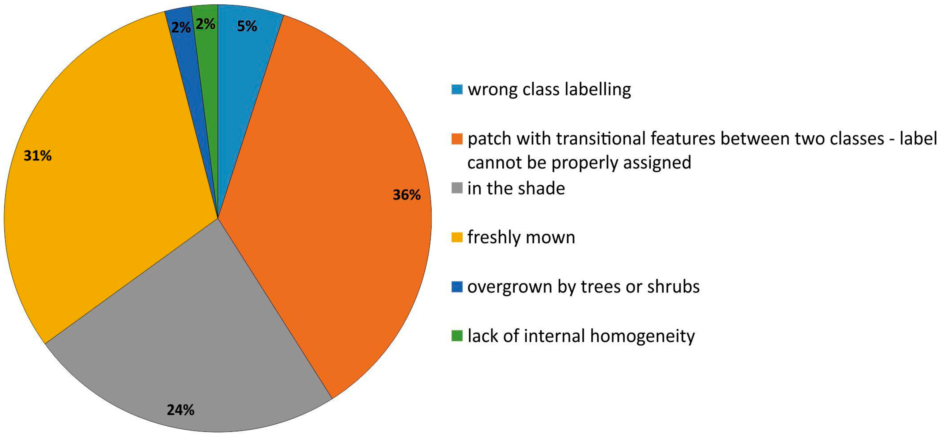
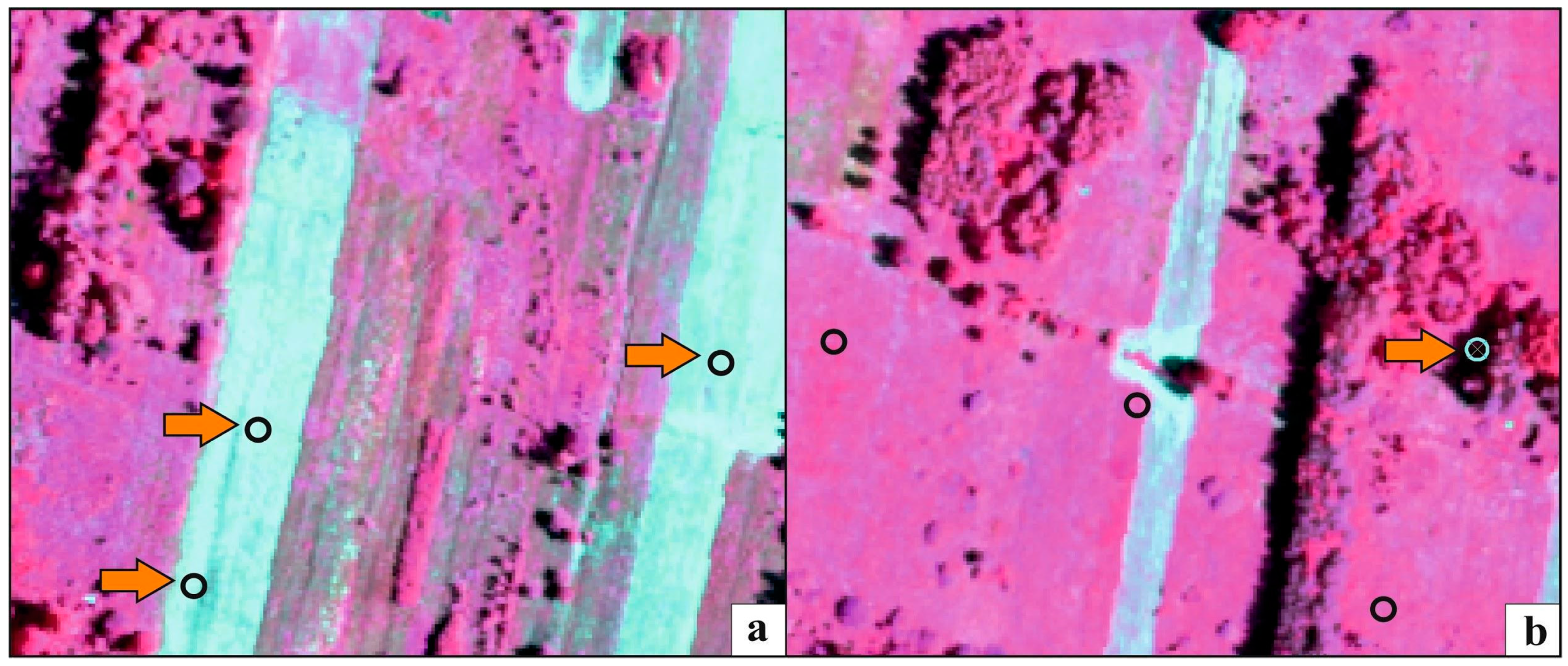
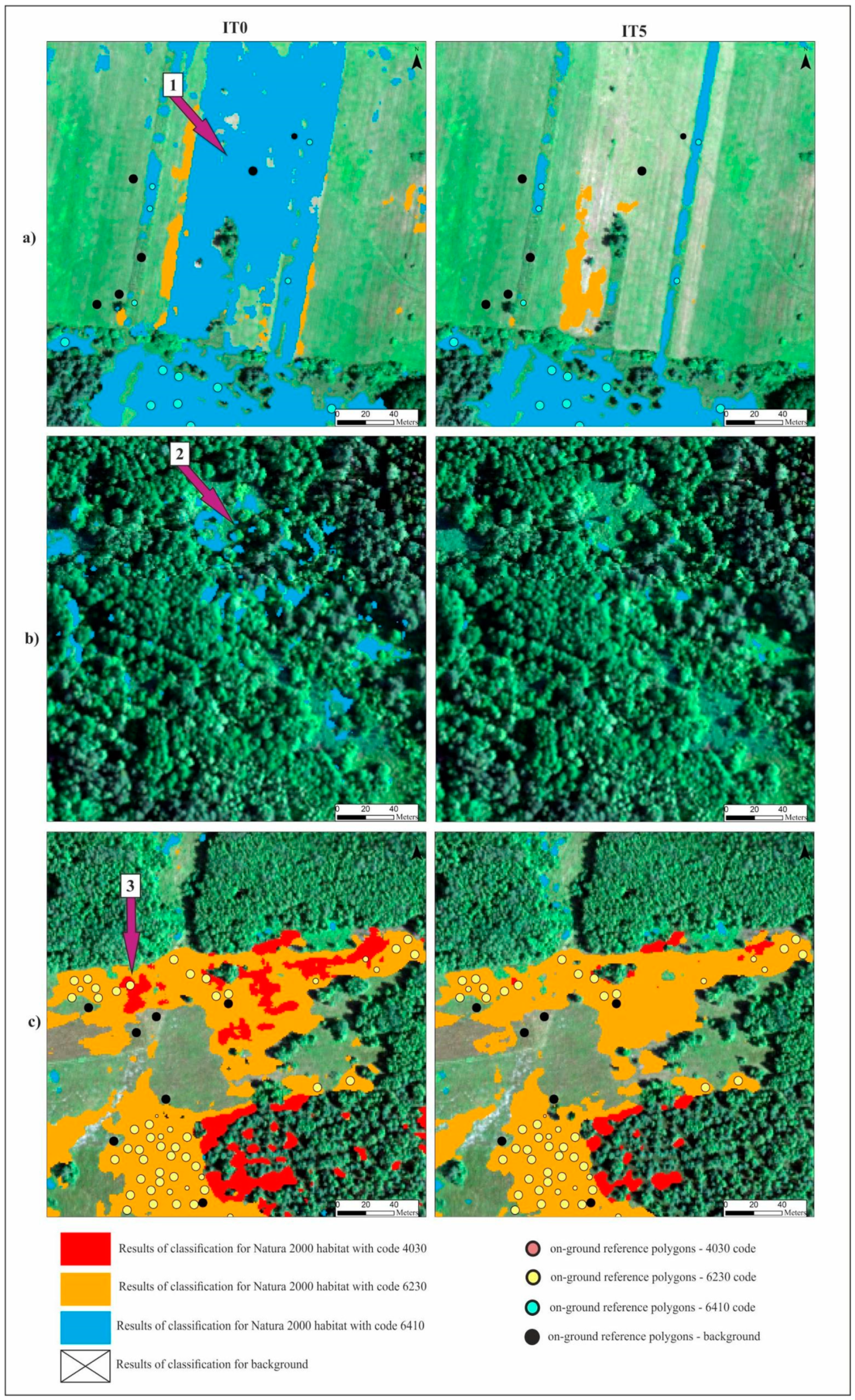
There were different underlying reasons for the polygons being artifacts in a visualization (Table 3, Figure 6). During the first iterations of the t-SNE analysis, the highest percentage of erroneous polygons were found for freshly mown areas (mainly class 6410), where young meadow vegetation (meadow sward) had not yet recovered (Figure 7a), and for areas located in the shade (mainly class 4030; Figure 7b). The presence of these erroneous polygons resulted in the overestimation of the membership of classes for other types of vegetation (background class). After they were removed from the database, the issue of overestimation was eliminated (Figure 8). Single polygons that were given incorrect class names were revealed in the course of the analysis of polygon attributes.
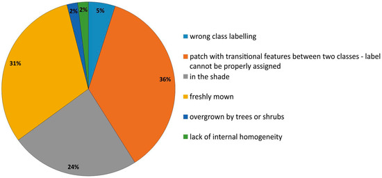
Figure 6.
The ratio of specific error types in reference dataset polygons identified during all iterations (IT0-IT5) of our workflow.

Figure 7.
Examples presenting the erroneous polygons identified during the t-SNE analysis, located in freshly mown areas (a) or in the shade (b). The orange arrow indicates erroneous polygons, which were removed from the on-ground reference dataset as a result of t-SNE analysis. The basic map—HySpex image in false color (CIR) acquired on July 7th, 2017.

Figure 8.
Comparison of the classification results for three Natura 2000 habitats (full fill) and background (transparent) made using RF algorithm for three selected fragments of study area (a–c) for IT0 and IT5. The basic map—HySpex image in RGB composition acquired on 7 July. Purple arrows indicate examples of errors on the resulting map from IT0, which were eliminated on the final result map (from IT5): 1—overestimation in freshly mown areas; 2—overestimation on trees, shrubs and in the shade; 3—overestimation of habitat with code 4030 in 6230 habitat patches.
Another reason for a given on-ground reference polygon being discovered as an artifact in the t-SNE visualization was the lack of internal homogeneity. This was revealed during the photointerpretation of the HySpex RGB and CIR composites, when one half of the on-ground reference polygon was placed in Natura 2000 habitat type 6230 and the other half in a compact patch of dry heaths (habitat with code 4030). Subsequent iterations of the t-SNE analysis enabled the identification of polygons located in vegetation patches, where analysis of the attributes showed the dominance of species not associated with the given Natura 2000 habitat, but with other analyzed habitats or the background. For example, patches of Natura 2000 habitat (code 6410) with a very high coverage (>50%) of the expansive grass species Calamagrostis epigejos, indicate late phase degradation of the habitat and should not be labeled as habitat 6410.
3.2. Effectiveness of Our Workflow
The t-SNE-based visual analysis resulted in choosing around 350–400 candidate reference polygons, that were identified as suspicious and were subjected to detailed assessment of their correctness. After the verification, 216 of them were found to contain errors of different kinds. Polygons identified as faulty were removed from the reference dataset, with ongoing classification and validation effort to validate the impact of changes on the quality of classification products. If our workflow is seen as a method to facilitate identification of faulty items in ground truth database, a critically important metric is its “error prediction” ability, that is the ratio of polygons that are identified as suspected vs. how many of them were found to be actually in error after investigation. It is obvious that this ratio shall be significantly better than finding these errors by chance or by systematic review of all polygons. That ratio in our study was around 50%. Unfortunately, we did not track all reference verification actions that confirmed the correctness of polygons—so we do not have exact data about how many polygons were verified to be correct. Also—because of many iterations of the analysis—there were cases that the same polygons were examined multiple times during various iterations. As we tried to afterwards reconstruct and collectively estimate amount of “correct checks”—our team concluded that minimum/conservative estimate of the amount of “polygon checks that turned correct” were not worse than 40–50%.
The workflow proposed in this paper assumed iterative nature of the process. In the course of the preliminary research, it was found that a single step analysis reveals only the most pronounced examples of misaligned polygons (characterized by the greatest spectral separability from the rest of the samples from a given class), while more subtle examples of erroneous polygons are identified only after the former are removed. This was found to be the preferred way to achieve almost perfect results, confirmed by final visualizations showing clusters characterized by significant homogeneity and distinctiveness between classes.
It is also noteworthy that out of the 216 errors identified and removed during 5 iterations, 133 were removed during IT1—becoming a 61.5% error removal rate during the first iteration, with the remaining 4 iterations delivering just below 10% each. So we might observe that, even though our workflow allowed us to perfect the reference data over 5 iterations until no further errors could be found, even just 1 round delivers quite substantial efficiency by removing the most outstanding and clearly visible errors, and by quickly identifying whole large groups of errors.
3.3. Results of the RF and AB Classification Obtained at Various Stages of the On-Ground Reference Dataset Modification
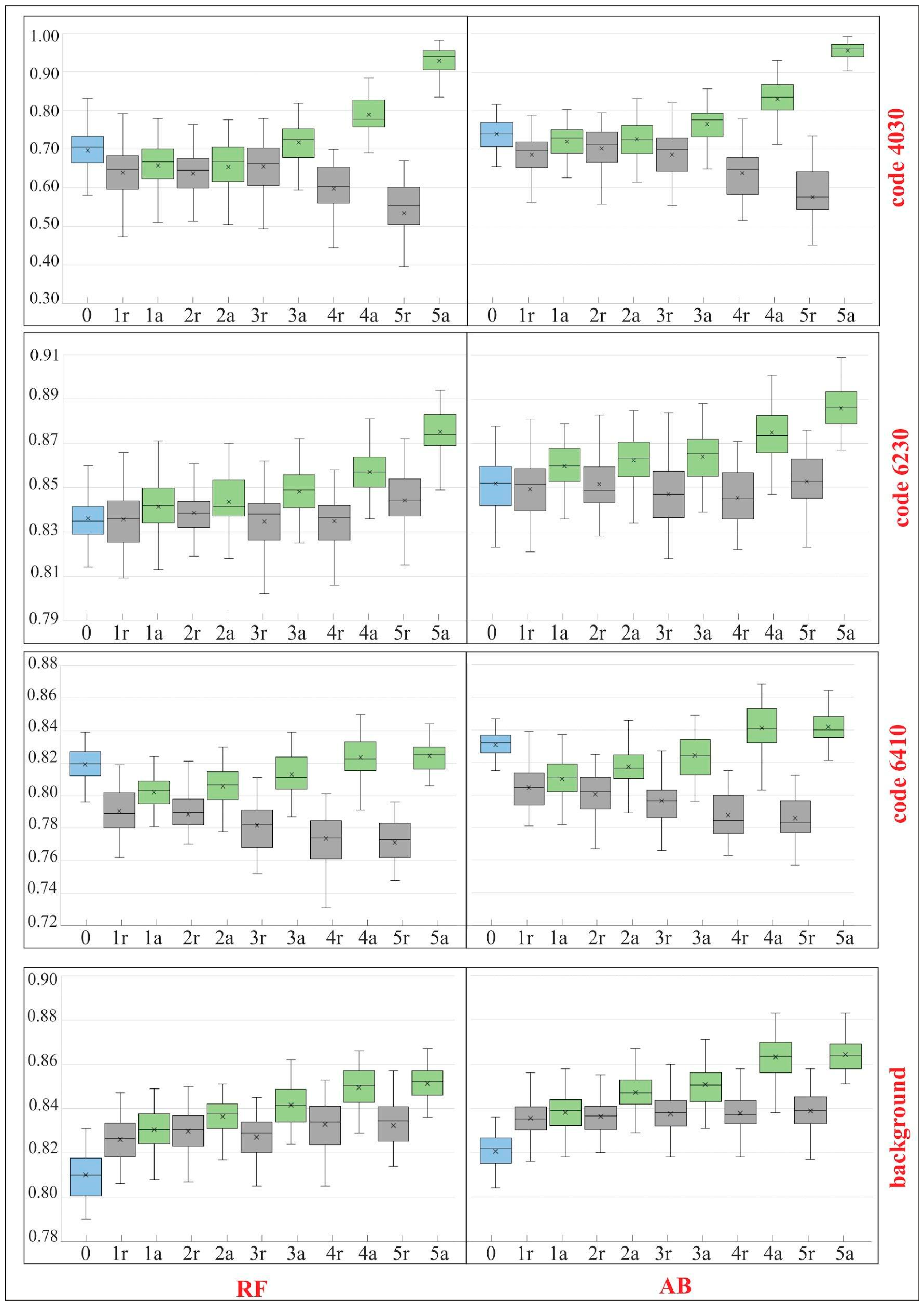
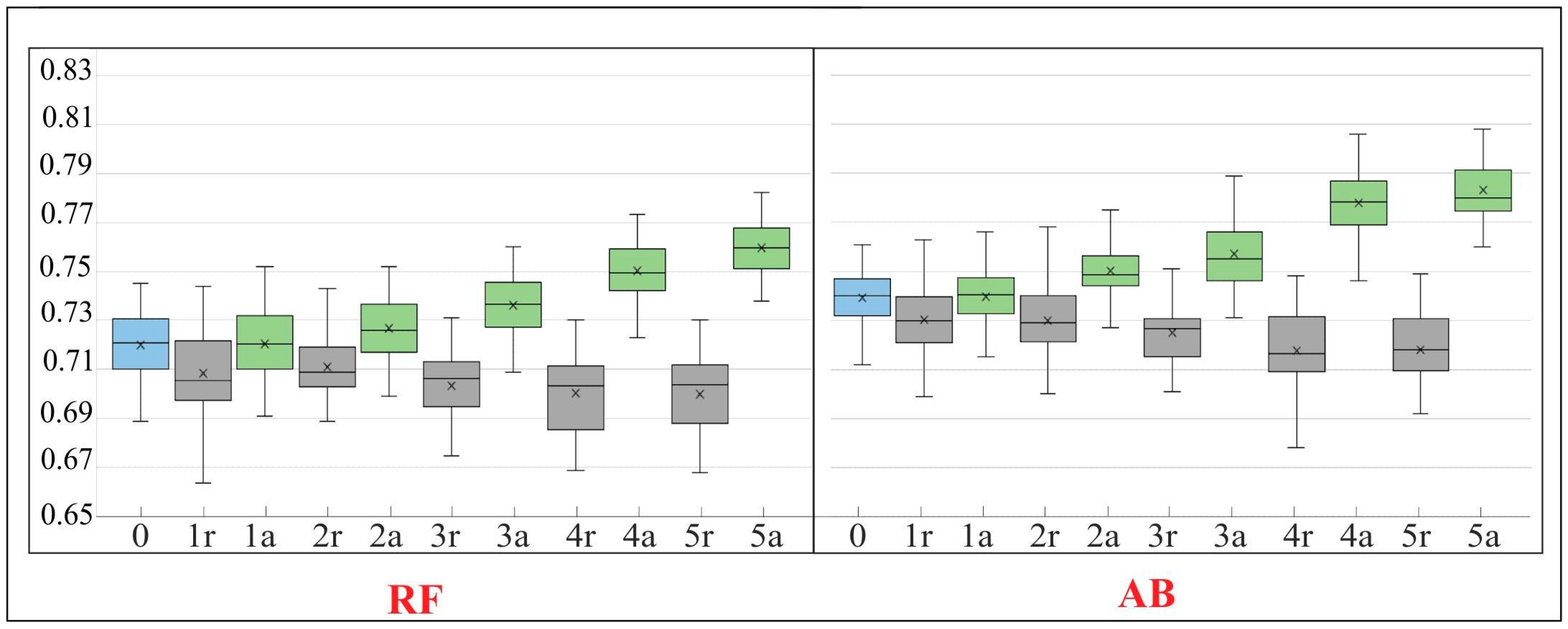
A total of six iterations (IT0–IT5) of the classification were carried out. The results clearly indicate that several modifications of the on-ground reference dataset, through the iterative t-SNE analysis, were advised to provide a significant, positive impact on the classification results as expressed by the analysis of accuracy measures, the comparison of spectral curves and visual evaluation of the output map. Comparing the results made on the dataset cleaned as a result of t-SNE analysis with those made using a randomly modified dataset (1r vs. 1a, 2r vs. 2a, etc.) (Figure 9 and Figure 10), we see an increase in the classification accuracy measures using our workflow. In the last iteration of the analysis an increase in the value of all F1 measures ranging from 2% for background (for RF) to 40% for the habitat with code 4030 (for RF) (Figure 9). The global accuracy of the map, expressed by the Kappa coefficient, increased after cleaning the set for both classification algorithms by about 6% (Figure 10).
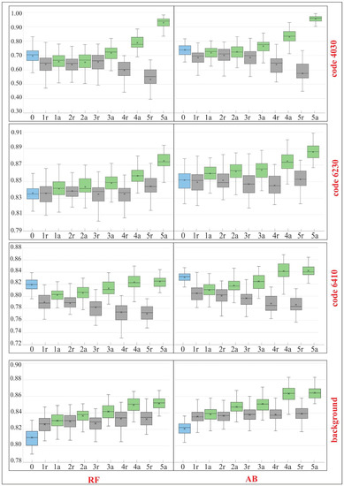
Figure 9.
Classification accuracies for F1 for Natura 2000 habitat (codes 4030, 6230, 6410) and the background in the subsequent iterations (IT0-IT5) of analysis—comparison of the results for the RF (random forest) and AB (AdaBoost) algorithms. The results were presented in the form of box-and-whisker plots which correspond to the results of 50 classifications. Whisker indicated min. and max. values, box represented interquartile range, the median was marked with the horizontal line and average value with the symbol “x”. IT0 was created on the unmodified reference dataset (blue boxes). IT5 is the final stage of our analysis. The main classifications after each iteration are labeled “a” (green boxes) (Step 1, Figure 2). The baseline classification with random removal of the same number of polygons are labeled “r” (grey boxes).
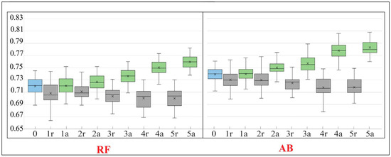
Figure 10.
The Kappa value in the subsequent iterations (IT0–IT5) of our workflow. For a detailed description of the figure see Figure 9.
3.4. Interpretation of Results
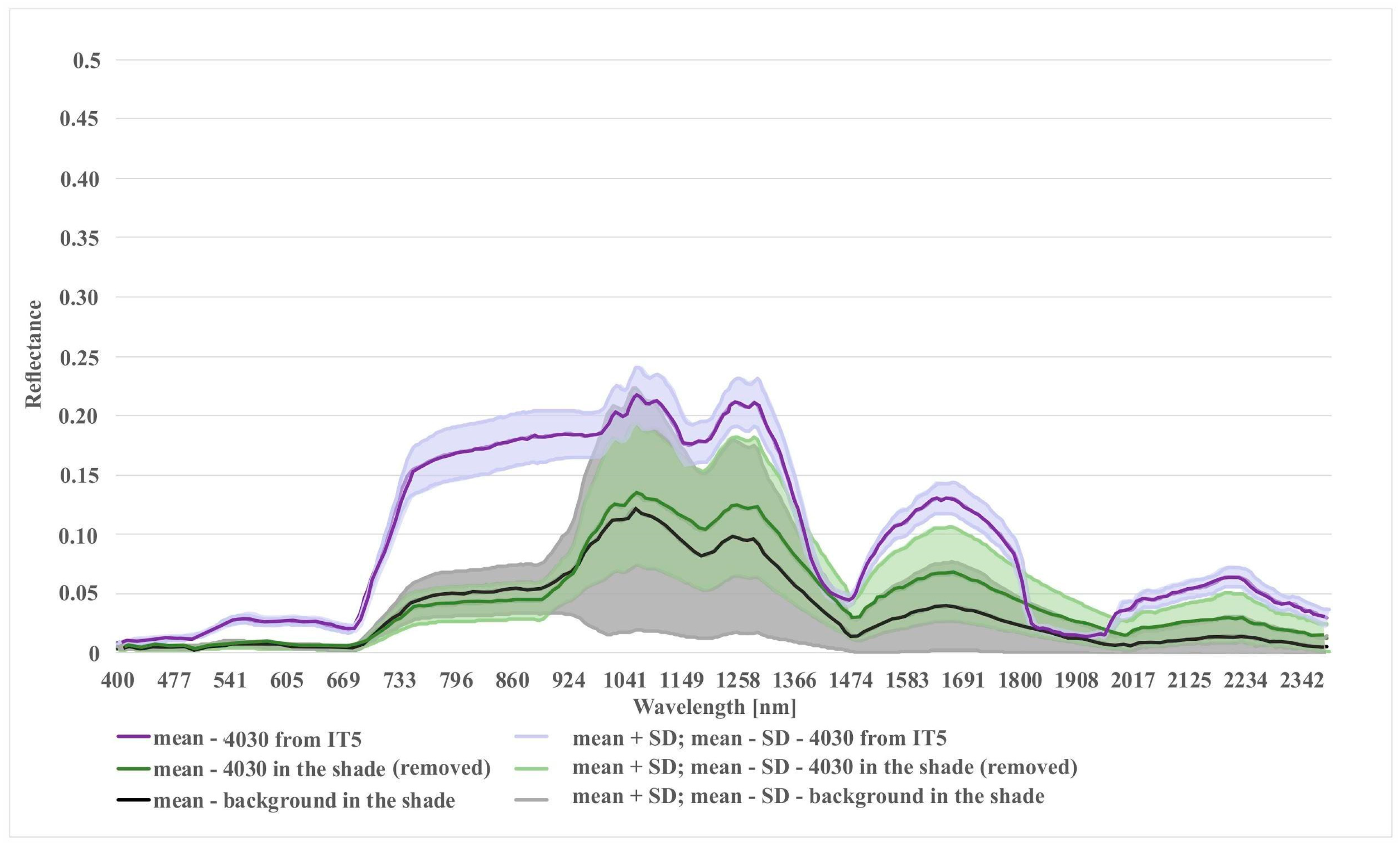
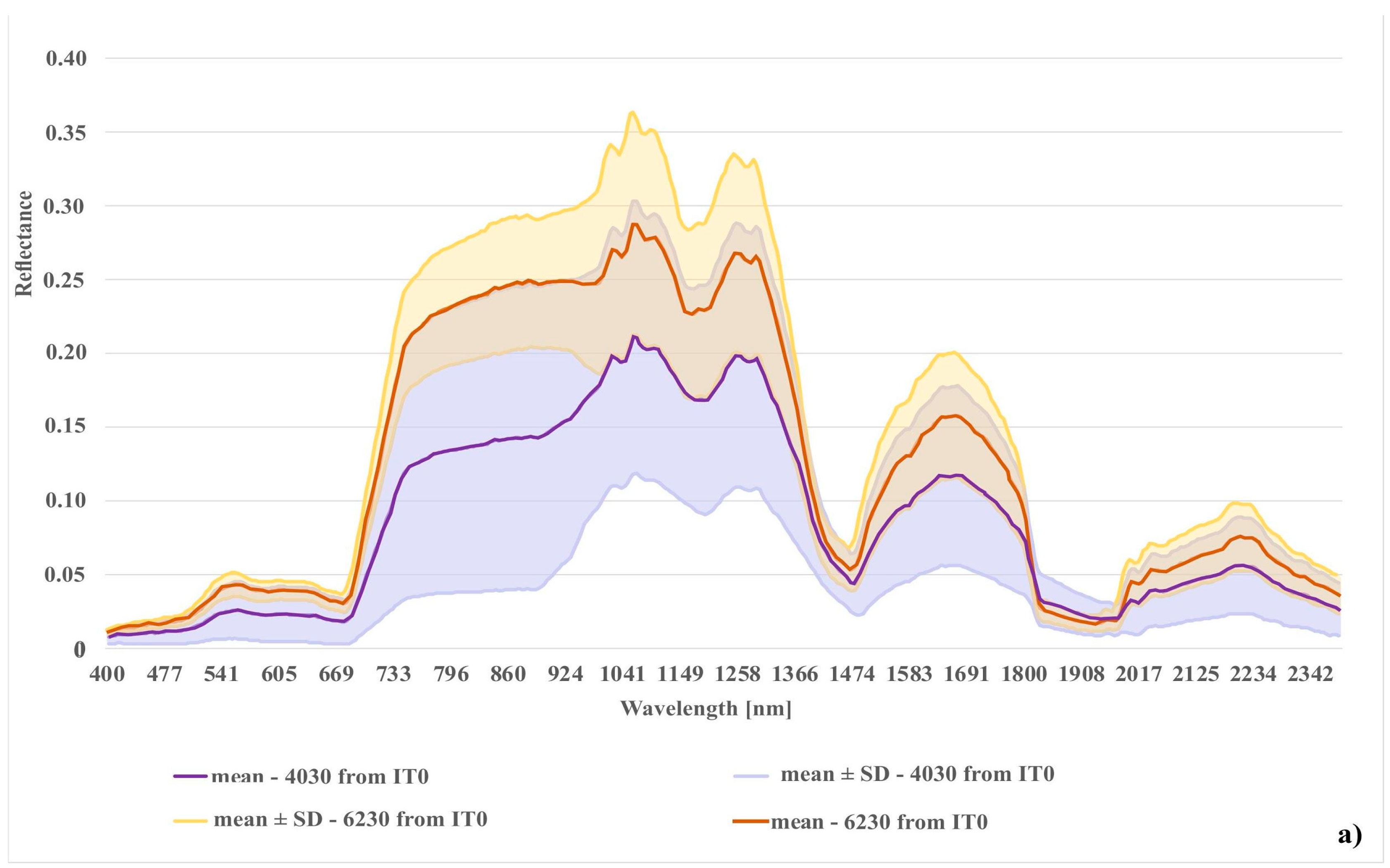
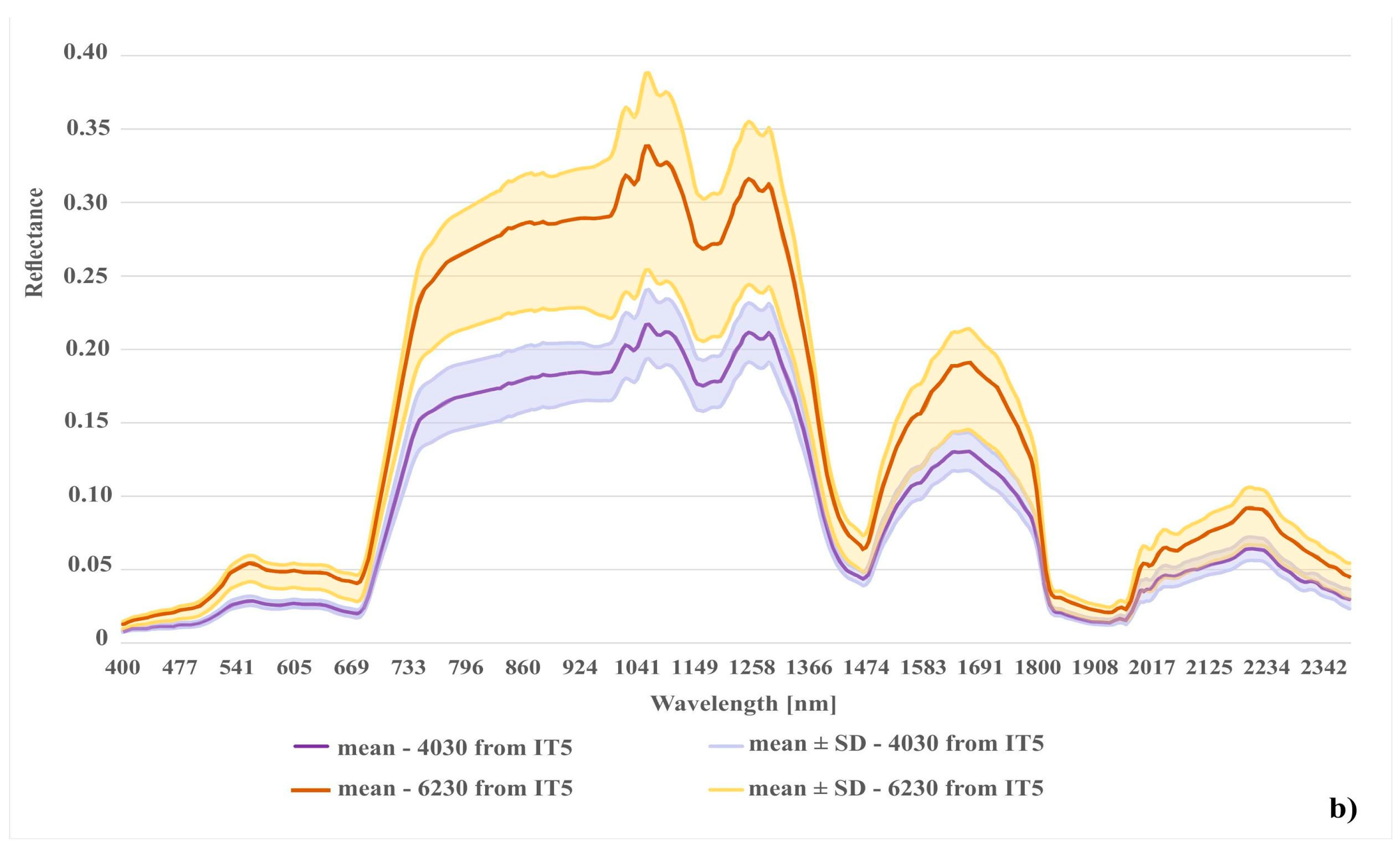
In the case of the habitat with code 4030, the highest percentage of artifact selected in the visualization was accounted for by polygons located in the shade. The comparison of the spectral curves clearly shows a high spectral similarity between polygons from the background class and polygons from habitat 4030 located in the shade (Figure 11). The visual assessment of the maps indicates that leaving the shaded polygons in class 4030 results in the overestimation in shaded areas of background such as forests and thickets (Figure 8). The highest increase in the F1 value was obtained during the IT4 and 5 (Figure 9; Table 5), when polygons having simultaneously the features of two classes (e.g. can be labeled as 4030 or 6230 code as well) were removed. These were the cases in which nearly identical species composition and, consequently, similar spectral features were observed. In addition, these similar polygons were labeled in the on-ground reference dataset as habitat 6230 and, at another time (by another author), as habitat 4030. Their removal from the on-ground reference dataset resulted in a decrease in the percentage of misclassified pixels between class 4030 and class 6230 (Table 5) and an increase in spectral distinctiveness between these Natura 2000 classes (Figure 12). Theoretically, these polygons could be labeled as a new transition class between 4030 and 6230, however, they were not sufficiently numerous to support model training so could not form their own separate class. The visual assessment of the map (from IT5) was also improved, showing almost no misclassifications and boundaries between patches similar to those observed in the field (cf. Figure 8, Table 4).
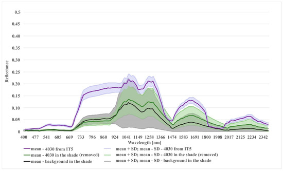
Figure 11.
Comparison of spectral curves for background class located in the shade and two different variants of Natura 2000 habitat (code 4030): (1) 4030 in shade (polygons removed after t-SNE analysis); (2) 4030 from the last iteration (IT5).

Table 5.
Comparison of the classification confusion matrices before (IT0) and after our workflow (IT5). Number of pixels were normalized to percentages. Each table cell contains results for both classifiers (RF/AB).


Figure 12.
Comparison of spectral curves created for two Natura 2000 habitat (codes 6230 and 4030); (a) spectral curves created from the unmodified reference dataset (IT0); (b) spectral curves created from final reference dataset (IT5).
When analyzing the results obtained for class with code 6230, we can observe a gradual systematic increase in mean F1 values relative to IT0 and difference between values using the dataset modified as a result of t-SNE analysis with those made using a randomly modified dataset. The removal of erroneous polygons from this class contributed to the reduction in the percentage of misclassified pixels between classes 6230 and 4030 (Table 5) and the increase in spectral distinctiveness between these classes (Figure 12). In addition, the percentage of misclassified pixels between classes 6230 and 6410 and the background also decreased. As in the case of class 4030, the producer’s accuracy and the user’s accuracy obtained with mean Kappa values were also improved (Table 5).
Different results were obtained for class 6410. The modifications to the on-ground reference dataset in this class did not bring the expected results. In the case of the RF algorithm, no increase in the mean F1 values was observed in relation to the unmodified on-ground reference dataset (IT0). In the case of the AB algorithm, the increase was small (Figure 9). The lack of improvement can be explained by the analysis of the error matrix (Table 5) which shows the main problem of misclassified pixels between class 6410 and the background. The percentage of misclassified pixels was not reduced in the subsequent iterations of the analysis, because the background class was not subjected to t-SNE analysis, and the types of vegetation constituting the background include vegetation patches characterized by high spectral similarity to class 6410 (Table 1). Errors 6410 class polygons located at recently mown sites were removed from the dataset during iterations 1–3. The validity of the decision to remove them from further analyses is additionally confirmed by the visual assessment of the classification map. Map obtained in the IT0 shows a very high overestimation of class 6410 in patches of mown vegetation belonging to the background class. While on the final map (from IT5), this overestimation disappears (Figure 8). The rationale for removing this type of error is confirmed by spectral curves created for mown versus unmown 6410 and other mown vegetation patches belonging to the background. The curves (Figure 13) show that this operation increased the internal homogeneity and distinctiveness between classes. The comparison of the map prepared based on the unmodified on-ground reference dataset and the map prepared based on the on-ground reference dataset after its last modification showed significant improvements in the distribution of habitat patches with code 6410 (Figure 8).
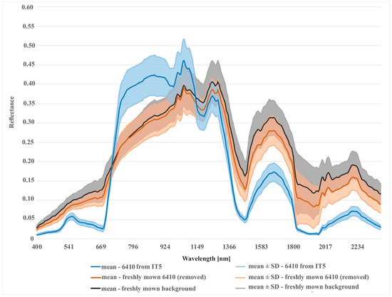
Figure 13.
Comparison of spectral curves for background class located in the freshly mown areas and two different variants of Natura 2000 habitat (code 6410): (1) 6410 in freshly mown areas (polygons removed after t-SNE analysis); (2) 6410 from last iteration (after removing of all detected errors).
For background, even though the reference polygons belonging to this class were not included in the t-SNE analysis, a systematic increase in the F1 values compared to first iteration and our baseline dataset was observed (Figure 9 and Figure 10).
The visual botanical map assessment showed a significant improvement in the classification results after the application of the entire t-SNE procedure. Classifications carried out on the unmodified on-ground reference dataset resulted in the overestimation of all Natura 2000 habitat classes relative to the background. This was most evident for class 6410, for which relatively large areas of other types of freshly mown vegetation patches or arable fields were misclassified as the habitat in question (Figure 8). Habitat overestimation was also observed in the shade and in patches of other types of vegetation with floristic composition similar to the Natura 2000 habitats. In the case of Natura 2000 habitat types 6230 and 4030, where agricultural use was sporadic, the overestimation concerned mainly mixing between two classes in patches of other plant communities of similar physiognomy, in areas overgrown with shrubs or trees, or otherwise shaded areas (Figure 8). It should be emphasized that limiting the total area of patches, which is visible on the resulting map from the last iteration, meant a favorable reduction in the overestimation of the surface of the studied Natura 2000 habitats. Visual botanical assessment demonstrated that due to the modification of the on-ground reference dataset after t-SNE analysis, a good quality map was obtained, on which the distribution and size of analyzed Natura 2000 habitats patches was close to reality.
4. Discussion
4.1. Evaluation of the t-SNE Algorithm Applicability to the Improvement of the On-Ground Reference Dataset Quality
The results achieved in the study indicate a significant potential of our workflow to improve the quality of on-ground reference datasets. Iteratively applied, not only reduces spectral variability within a given class, but also increases spectral differences between classes (Figure 11, Figure 12 and Figure 13). The analysis led to the successful discrimination between patches with the same dominants, i.e. some forms of Natura 2000 habitats with codes 6230 and 4030, where, according to botanical criteria, affiliation to a given Natura 2000 habitat type was determined based on plants with low cover-abundance (below 20%), thus difficult to distinguish by remote sensing methods. The added value of the experiment is not only to obtain a fully reliable and class-specific spectral profile, but also to learn the intraclass variation of each band, which demonstrates the natural spectral variability of a given class. Knowledge of this aspect can be very useful not only at the stage of sampling design planning (land cover classes with greater variability will require more samples) but also interpretation of classification results. The visualizations resulting from our workflow (Figure 4) enabled the effective identification of erroneous on-ground reference polygons. The most clearly visible errors were detected on the visualizations during IT0. Those are mostly polygons where disturbing factors (such as shading, mowing) are present, which decrease the spectral separation between individual Natura 2000 habitats. Also, the spectral features of such polygons are more similar to background polygons with the same features (for example, shadowed or mown polygons already present in our background class). This is evident in the case of polygons representing Natura 2000 habitat with code 4030 located in the shade and type 6410 in freshly mown patches (Figure 11 and Figure 13). In such a situation, polygons from different classes may form one or more separate clusters, often located far from their main (or dominant) cluster(s).
It is important to note that the effectiveness of our workflow depends, to a large extent, on the spectral features of the classes analyzed together and on the number of errors in the database. The authors’ experience to date, accumulated during HabitARS project [11], indicates that for naturally heterogeneous classes the identification of errors is much harder than for more homogeneous ones, such as Natura 2000 habitat 4030. A large proportion of erroneous polygons within a class also increases apparent variability within class, which above some threshold can also make their detection harder. Therefore, when planning to perform the t-SNE analysis, the experimental methodology should be adjusted to specific characteristics of the dataset. It is recommended to limit the number of classes analyzed simultaneously, especially when they are characterized by large heterogeneity and low inter-class separability, as this may make it difficult to obtain clear visualizations. At first, the number of analyzed classes can be artificially limited; additional classes may be added one by one after most errors have been iteratively identified and removed from a given set of classes. Problems with the interpretation of the t-SNE analysis may also arise when a given class is naturally quite broad (it can be formed from different species of herbaceous plants); such classes may in fact consist of a number of smaller subclasses.
The visualization methodology is also a very important aspect of the interpretative capacity of the t-SNE algorithm. Since the visualizations are not deterministic, and some t-SNE algorithm settings can influence the visual output considerably, it is recommended to experiment a bit with the settings until a suitable visualization is obtained. It is strongly recommended to assess the impact of different perplexity values. Perplexity settings determine how many neighboring points (or samples) are taken into account when solving the optimal visualization layout. Often, the value of perplexity has a fairly significant impact on the interpretability of a visualization as different aspects of the dataset appear enhanced or suppressed (e.g. some settings expose more local structure of the data). Typically, the best perplexity settings are influenced by global properties of the dataset, such as the total number of samples, the number of classes, the number of samples per class, as well as the internal variability of data. Therefore, since it is not easy to give specific guidelines as to preferred values, it is recommended to try a few settings at the outset. Once good settings are determined, they can be typically reused with the same dataset with good results.
For workflows involving repeated comparisons of multiple visualizations of the same dataset, the consistency between visualizations is a critical aspect enabling visual analysis by human experts. By default, t-SNE initializes the global structure of 2D visualization in a slightly unpredictable way. As the global structure is not preserved, multiple visualizations—even for the same or very similar dataset—may have a similar local structure, whereas the global structure layout may vary greatly (for example, visualizations may be mirrored, flipped along the horizontal or vertical axis, or laid out in otherwise different way). Even though the local structure of the dataset is typically well represented, such global layout changes will hamper the interpretability and comparison of such visualizations by experts. Therefore, it is strongly recommended to select t-SNE settings that perform a stable/repeatable initial layout, using a globally-stable transformation. The most common solution is to initialize the t-SNE layout with a PCA-transformed dataset.
4.2. Impact of the On-Ground Reference Dataset Modification on the Results of Classification of Selected Natura 2000 Habitats
The iterative t-SNE analysis significantly improved the classification results, expressed both by the statistical significance of the differences in the Kappa and F1 values (Table 5; Figure 9 and Figure 10) and by the visual evaluation of the results by botanists, who collected on-ground reference polygons and knew the study area well. This made it possible to mitigate the negative impact of the lack of correspondence in the time frames for the acquisition of on-ground reference data and remote sensing data. This also provides new opportunities for the use of data originating from varying sources, whose quality could not thus far be verified. The impact of existing errors in the on-ground reference dataset on the classification results is highly dependent on the Natura 2000 habitat type.
When comparing the F1 results obtained in this study for individual Natura 2000 habitats with other published reports, it can be concluded that the results obtained for data acquired during one airborne collection, using only the first 30 MNF channels and the on-ground reference database improved by the t-SNE analysis, are comparable or even better than the results obtained by other researchers. In the case of Natura 2000 habitat with code 4030, the maximum F1 value known from the literature is 0.83, where classifications were conducted on high-resolution color orthophotography and digital surface models (DSMs) from an unmanned aerial vehicle UAV [37]. For comparison, the maximum F1 value for class 4030 obtained within the scope of the presented work was 0.99 (Figure 9). Analyzing the results obtained for Natura 2000 habitat with code 6230, similar results were produced with F1 values obtained using data acquired from an unmanned aerial vehicle UAV [37], i.e., 0.92 and 0.93, respectively. High F1 values were also obtained in this study for habitat code 6410, with a maximum value of 0.87. For comparison, the maximum F1 values reported in the literature range from 0.46, where classification was carried out using a RapidEye time series [38,39], to 0.98, where classifications were carried out using as many as 21 observations of an intra-annual time series acquired by a multi-spectral (RapidEye) and a synthetic aperture radar (TerraSAR-X) satellite system [40]. Lower F1 values (0.69) were also obtained using full-waveform airborne laser scanning [41]. The obtained results clearly indicate that the improvement of the on-ground reference dataset using the t-SNE algorithm coupled with classification using a single hyperspectral mosaic is an alternative to the use of other approaches, including single sources (e.g., airborne laser scanning (ALS) [31]), multiple sources and using multi-temporal data fusion.
The RF algorithm is commonly considered as largely resistant to noisy and mislabeled training data [3,9,27,28,42]. According to some studies, even features containing noise levels as high as 30% result in a decrease in Kappa accuracy in the range of 10%, which is considered a very moderate decrease [43]. Our results confirm the relative insensitivity of RF to noisy (errors) data. With a level of error about 15%, Kappa accuracy decreased by only about 6% (Figure 9 and Figure 10). The results obtained with the AB algorithm indicate that the classifier also proved to be relatively resistant to noise (Figure 8 and Figure 9). However, when we compare the classification results (Figure 9 and Figure 10) made on a randomly modified on-ground reference dataset (with identical number of training and validation polygons in each class) with those made on the data modified as a result of t-SNE analysis, a statistical significant increase in the value of Kappa coefficient is visible already from the first iteration (for both RF and AB) (Figure 9 and Figure 10). Comparing the results obtained after the last iteration of t-SNE analysis, an increase in Kappa value was observed by about 6%, relative to the classification results obtained using a randomly modified reference dataset.
Furthermore, a visual assessment of the results clearly indicates significant differences in the mapping effectiveness before IT0 and after the final improvement (IT5) of the on-ground reference dataset (Figure 8). Our analysis shows that an assessment of the classification accuracy alone, without an assessment performed by a botanist familiar with the field data, may not be sufficient. In particular, that in such heterogeneous areas as represented by study area (Natura 2000 site “Dolina Krasnej”), it is practically impossible to collect a sufficient number of polygons of background which would fully represent the variability of spectral features within the study area. For this reason, the impact of noise in the data on the classification results may be underestimated, and the resulting map may consequently not be suitable for practical use. It should also be noted that in the open literature, noise in the data often concerns only training polygons and classes that are quite easy to distinguish by a classifier. Researchers point out that in other situations the impact of noise in the data may be more significant [9]. At the same time, many different accuracy measures are compared in the literature to assess the resistance of classifiers to noise in reference data. According to [27], much depends on which measure is used to assess the resistance of a given classification methodology to noise and sometimes contradictory results are obtained even on the same data.
5. Conclusions
Our workflow supports effective detection and correction of errors in ground truth reference database. We use visual analysis of t-SNE based plots to identify the subset of reference database having specific visual artifacts and patterns (Table 3), correlated with significant probability of containing errors. Identified reference polygons are candidate suspects for additional inspection and verification. In our testing dataset, more than half of candidate reference polygons identified during the first iteration were found to contain errors.
In this work, each iteration of our error detection and correction was followed by classification and detailed validation to assess the impact of our workflow on classification results. It is possible however to use this process to find and fix reference errors before or even independently of any classification.
The results of our research suggest that such workflow is particularly effective when either: (a) an on-ground reference dataset was not synchronized in time to the acquisition of remote sensing data; (b) the information content of the reference database is scarce, possibly containing only the class label, and lacking any redundancy (e.g., detailed information on species composition, field notes, photographs, or other attributes are missing), thus preventing any ways to verify its correctness or assess its quality; (c) an on-ground reference dataset is particularly prone to contain errors or is expected to be of inferior quality, for example when it is integrated from multiple sources, was collected by other parties or in conditions we have no sufficient control or knowledge, (d) in work regimes where field work is particularly difficult, costly, the study area is remote or hardly accessible, or the time window to collect reference is already closed—while there is still potential and need to increase the quality of the data by intensive post-processing/analysis.
Author Contributions
Conceptualization, A.H.-D. and D.K.; Investigation, A.H.-D. and A.K.; Methodology, A.H.-D. and D.K.; Project administration, D.K.; Resources, A.K.; Software, A.K.; Supervision, D.K.; Validation, A.K.; Visualization, A.H.-D. and A.K.; Writing—original draft, A.H.-D., A.K. and D.K.; Writing—review and editing, D.K. All authors have read and agreed to the published version of the manuscript.
Funding
The study was co-financed by the Polish National Centre for Research and Development (NCBR) and MGGP Aero under the programme “Natural Environment, Agriculture and Forestry” BIOSTRATEG II.: The innovative approach supporting monitoring of non-forest Natura 2000 habitats, using remote sensing methods (HabitARS), project number: DZP/BIOSTRATEG-II/390/2015. The Consortium Leader is MGGP Aero. The project partners include the University of Lodz, the University of Warsaw, Warsaw University of Life Sciences, the Institute of Technology and Life Sciences, the University of Silesia in Katowice, Warsaw University of Technology.
Conflicts of Interest
The authors declare no conflict of interest.
References
- Foody, G.M.; Pal, M.; Rocchini, D.; Garzon-Lopez, C.; Bastin, L. The sensitivity of mapping methods to reference data quality: Training supervised image classifications with imperfect reference data. ISPRS Int. J. Geo-Inf. 2016, 5, 199. [Google Scholar] [CrossRef]
- Lillesand, T.M.; Kiefer, R.W. Remote Sensing and Image Interpretation, 3rd ed.; John Wiley & Sons: New York, NY, USA, 1994. [Google Scholar]
- Mellor, A.; Boukir, S.; Haywood, A.; Jones, S. Exploring issues of training data imbalance and mislabelling on random forest performance for large area land cover classification using the ensemble margin. ISPRS J. Photogramm. Remote Sens. 2015, 105, 155–168. [Google Scholar] [CrossRef]
- Costa, H.; Foody, G.M.; Jiménez, S.; Silva, L. Impacts of species misidentification on species distribution modeling with presence-only data. ISPRS Int. J. Geo-Inf. 2015, 4, 2496–2518. [Google Scholar] [CrossRef]
- Mather, P.M. Computer Processing of Remotely-Sensed Images: An Introduction, 3rd ed.; John Wiley and Sons: Chichester, UK, 2004. [Google Scholar]
- Congalton, R.G.; Green, K. Assessing the Accuracy of Remotely Sensed Data: Principles and Practices; CRC Press: Boca Raton, FL, USA, 2008. [Google Scholar]
- Foody, G.M.; Mathur, A.; Sanchez-Hernandez, C.; Boyd, D.S. Training set size requirements for the classification of a specific class. Remote Sens. Environ. 2006, 104, 1–14. [Google Scholar] [CrossRef]
- Ge, Y.; Bai, H.; Wang, J.; Cao, F. Assessing the quality of training data in the supervised classification of remotely sensed imagery: A correlation analysis. J. Spat. Sci. 2012, 57, 135–152. [Google Scholar] [CrossRef]
- Pelletier, C.; Valero, S.; Inglada, J.; Champion, N.; Sicre, C.M.; Dedieu, G. Effect of training class label noise on classification performances for land cover mapping with satellite image time series. Remote Sens. 2017, 9, 173. [Google Scholar] [CrossRef]
- Guo, L. Margin Framework for Ensemble Classifiers. Application to Remote Sensing Data. Ph.D. Thesis, University of Bordeaux, Bordeaux, France, 2011. [Google Scholar]
- Kopeć, K.; Wylazłowska, J.; Niedzielko, J.; Jarocińska, A.; Borzuchowski, J.; Piórkowski, H.; Błońska, A.; Niedzielko, M.; Halladin-Dąbrowska, A.; Michalska-Hejduk, D.; et al. Auxiliary work in WP3 under the programme “Natural Environment, Agriculture and Forestry” BIOSTRATEG II.: The innovative approach supporting monitoring of non-forest Natura 2000 habitats, using remote sensing methods (HabitARS). Unpublished work.
- Ramaswamy, S.; Rastogi, R.; Shim KAIST, K. Efficient algorithms for mining outliers from large data sets. In Proceedings of the 2000 ACM SIGMOD International Conference on Management of Data, Dallas, TX, USA, 15–18 May 2000. [Google Scholar]
- Liu, F.T.; Ting, K.M.; Zhou, Z.-H. Isolation-based anomaly detection. ACM Trans. Knowl. Discov. Data 2012, 6, 3. [Google Scholar] [CrossRef]
- Breunig, M.M.; Kriegel, H.-P.; Ng, R.T.; Sander, J. LOF: Identifying density-based local outliers. In Proceedings of the 2000 ACM SIGMOD International Conference on Management of Data, Dallas, TX, USA, 15–18 May 2000. [Google Scholar]
- Büschenfeld, T.; Ostermann, J. Automatic refinement of training data for classification of satellite imagery. In Proceedings of the PISPRS Annals of the Photogrammetry, Remote Sensing and Spatial Information Sciences, Melbourne, Australia, 25 August–1 September 2012. [Google Scholar]
- Kavzoglu, T. Increasing the accuracy of neural network classification using refined training data. Environ. Model. Softw. 2009, 24, 850–858. [Google Scholar] [CrossRef]
- Mather, P.M. Computational Methods of Multivariate Analysis in Physical Geography; John Wiley and Sons: Chichester, UK, 1976. [Google Scholar]
- Van Der Maaten, L.; Hinton, G. Visualizing data using t-SNE. J. Mach. Learn. Res. 2008, 9, 2579–2605. [Google Scholar]
- Zhang, J.; Chen, L.; Zhuo, L.; Liang, X.; Li, J. An efficient hyperspectral image retrieval method: Deep spectral-spatial feature extraction with DCGAN and dimensionality reduction using t-SNE-based NM hashing. Remote Sens. 2018, 10, 271. [Google Scholar] [CrossRef]
- Zhong, Z.; Li, J.; Ma, L.; Jiang, H.; Zhao, H. Deep residual networks for hyperspectral image classification. In Proceedings of the IEEE International Geoscience and Remote Sensing Symposium (IGARSS), Fort Worth, TX, USA, 23–28 July 2017. [Google Scholar]
- Dai, X.; Guo, S.; Li, X. Novel hyperspectral image classification method based on the t-SNE and AdaBoost algorithms. In Proceedings of the Association of American Geographers Annual Meeting, New Orleans, LA, USA, 10–14 April 2018. [Google Scholar]
- Zhang, L.; Zhong, Y.; Huang, B.; Gong, J.; Li, P. Dimensionality reduction based on clonal selection for hyperspectral imagery. IEEE Trans. Geosci. Remote Sens. 2007, 45, 4172–4186. [Google Scholar] [CrossRef]
- Halladin-Dąbrowska, A.; Kania, A.; Sławik, Ł.; Niedzielko, J.; Borzuchowski, J.; Wylazłowska, J.; Michalska-Hejduka, D.; Kopeć, D. The t-SNE Machine Learning Algorithm As A Novel Tool Supporting The Classification Of Non-forest Natura 2000 Habitats. In Proceedings of the Sixth International Conference on Remote Sensing and Geoinformation of Environment, Paphos, Cyprus, 26–29 March 2018. [Google Scholar]
- Kania, A. Interactive tool for real-time delivery of remote sensing based vegetation maps and support of botanical data collection. In Proceedings of the 10th International Conference on Ecological Informatics. Translating Ecological Data into Knowledge and Decisions in a Rapidly Changing World, Jena, Germany, 24–28 September 2018; pp. 59–60. [Google Scholar]
- Chan, W.; Spanhove, T.; Ma, J.; Vanden Borre, J.; Paelinckx, D.; Canters, F. Natura 2000 habitat identification and conservation status assessment with superresolution enhanced hyperspectral (CHRIS/PROBA) imagery. In Proceedings of the GEOBIA 2010-Geographic Object-Based Image Analysis, Ghent, Belgium, 29 June–2 July 2010. [Google Scholar]
- Folleco, A.; Khoshgoftaar, T.M.; Hulse, J.; Van Bullard, L. Identifying learners robust to low quality data. In Proceedings of the IEEE International Conference on Information Reuse and Integration, Las Vegas, NV, USA, 13–15 July 2008. [Google Scholar] [CrossRef]
- Rodriguez-Galiano, V.; Ghimire, B.; Rogan, J.; Chica-Olmo, M.; Rigol-Sanchez, J. An assessment of the effectiveness of a random forest classifier for land-cover classification. ISPRS J. Photogramm. Remote Sens. 2012, 67, 93–104. [Google Scholar] [CrossRef]
- Sun, B.; Chen, S.; Wang, J.; Chen, H. A robust multi-class AdaBoost algorithm for mislabeled noisy data. Knowl.-Based Syst. 2016, 102, 87–102. [Google Scholar] [CrossRef]
- Banfield, R.E.; Hall, L.O.; Bowyer, K.W.; Kegelmeyer, W.P. A Comparison of decision tree ensemble creation techniques. IEEE Trans. Pattern. Anal. Mach. Intell. 2007, 29, 173–180. [Google Scholar] [CrossRef]
- Dietterich, T.G. An experimental comparison of three methods for constructing ensembles of decision trees: Bagging, boosting, and randomization. Mach. Learn. 2000, 40, 139–157. [Google Scholar] [CrossRef]
- Sławik, Ł.; Niedzielko, J.; Kania, A.; Piórkowski, H.; Kopeć, D. Multiple flights or single flight instrument fusion of hyperspectral and ALS data? A comparison of their performance for vegetation mapping. Remote Sens. 2019, 11, 970. [Google Scholar] [CrossRef]
- ENVI API Programming Guide. Harris Geospatial Solutions Documentation Center. Available online: http://www.harrisgeospatial.com/docs/ProgrammingGuideIntroduction.html (accessed on 8 February 2019).
- Millard, K.; Richardson, M. Wetland mapping with LiDAR derivatives, SAR polarimetric decompositions, and LiDAR-SAR fusion using a random forest classifier. Can. J. Remote Sens. 2013, 39, 290–307. [Google Scholar] [CrossRef]
- Van Der Maaten, L.; Courville, A.; Fergus, R.; Manning, C. Accelerating t-SNE using tree-based algorithms. J Mach. Learn. Res. 2014, 15, 3221–3245. [Google Scholar]
- Vegetation Classification Studio Software, Version 2.13/hb. Available online: http://www.definity.pl/vcs (accessed on 5 September 2019).
- Cohen, J. A Coefficient of Agreement for Nominal Scales. Educ. Psychol. Meas. 1960, 20, 37–46. [Google Scholar] [CrossRef]
- Gonçalves, J.; Henriques, R.; Alves, P.; Sousa-Silva, R.; Monteiro, A.T.; Lomba, Â.; Marcos, B.; Honrado, J. Evaluating an unmanned aerial vehicle-based approach for assessing habitat extent and condition in fine-scale early successional mountain mosaics. Appl. Veg. Sci. 2016, 19, 132–146. [Google Scholar] [CrossRef]
- Buck, O.; Millán, V.E.G.; Klink, A.; Pakzad, K. Using information layers for mapping grassland habitat distribution at local to regional scales. Int. J. Appl. Earth Obs. Geoinf. 2015, 37, 83–89. [Google Scholar] [CrossRef]
- Stenzel, S.; Feilhauer, H.; Mack, B.; Metz, A.; Schmidtlein, S. Remote sensing of scattered natura 2000 habitats using a one-class classifier. Int. J. Appl. Earth Obs. Geoinf. 2014, 33, 211–217. [Google Scholar] [CrossRef]
- Schuster, C.; Schmidt, T.; Conrad, C.; Kleinschmit, B.; Förster, M. Grassland habitat mapping by intra-annual time series analysis -Comparison of RapidEye and TerraSAR-X satellite data. Int. J. Appl. Earth Obs. Geoinf. 2015, 34, 25–34. [Google Scholar] [CrossRef]
- Zlinszky, A.; Schroiff, A.; Kania, A.; Deák, B.; Mücke, W.; Vári, Á.; Székely, B.; Pfeifer, N. Categorizing grassland vegetation with full-waveform airborne laser scanning: A feasibility study for detecting natura 2000 habitat types. Remote Sens. 2014, 6, 8056–8087. [Google Scholar] [CrossRef]
- Breiman, L. Random Forests. Mach. Learn. 2001, 45, 5–32. [Google Scholar] [CrossRef]
- Agjee, N.H.; Mutanga, O.; Peerbhay, K.; Ismail, R. The Impact of Simulated Spectral Noise on Random Forest and Oblique Random Forest Classification Performance. J. Spectrosc. 2018, 2018, 8316918. [Google Scholar] [CrossRef]
© 2019 by the authors. Licensee MDPI, Basel, Switzerland. This article is an open access article distributed under the terms and conditions of the Creative Commons Attribution (CC BY) license (http://creativecommons.org/licenses/by/4.0/).


